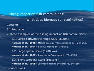
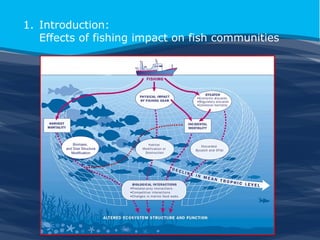
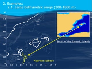
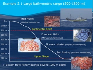
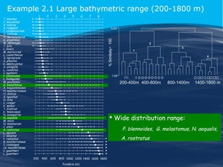
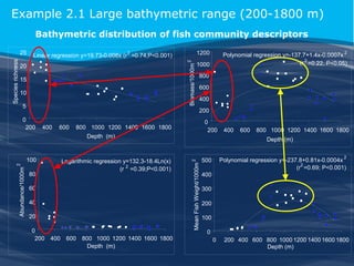
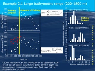
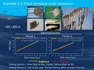
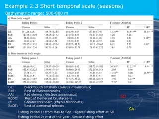
call girls in Kamla Market (DELHI) 🔝 >༒9953330565🔝 genuine Escort Service 🔝✔️✔️
Fishing impact on fish communities
1. Fishing impact on fish communities:
What does biomass (or size) tell us?
Joan Moranta
Thesis: Deep western Mediterranean demersal fish communities
Spanish Institute of Oceanography
Palma de Mallorca, Balearic Islands, Spain
School of Ocean Science
Menai Bridge, Anglesey, UK
2. Fishing impact on fish communities:
What does biomass (or size) tell us?
Contents :
1.Introduction
2.Three examples of the fishing impact on fish communities
2.1. Large bathymetric range (200-1800m)
Moranta et al. (1998). Marine Ecology Progress Series 171, 247-259.
Moranta et al. (2004). Scientia Marina 68, 141-152.
2.2. Large spatial scale (1200 km)
Moranta et al. (2007). Progress in Oceanography 72, 63-83.
2.3. Short temporal scale (seasons)
Moranta et al. (2008). Journal of Marine Systems 71, 346-366.
3.Conclusions
4. 1. Introduction:
Something to compare with (CONTROL)
The Baseline Scenario
Pristine Ecosystem
Few ‘unfished’ control sites are now available for
study, and these are at the scale of small areas
such as individual reefs rather than ecosystems
(Jennings & Kaiser 1998)
Absence of Fishing
Marine Reserves
↑ Number of species
↑ Abundance of species
↑ Sizes at shallow depth
5. 2. Examples:
2.1. Large bathymetric range (200-1800 m)
42
41.5
400
1000
41
2000
40.5
40
Menorca
South of the Balearic Islands
Mallorca
39.5
Eivissa
39
600
Formentera
38.5
800
400
1000
38
Algeriana subbasin
2000
0
0.5
1
1.5
2
2.5
3
3.5
4
4.5
5
6. Example 2.1 Large bathymetric range (200-1800 m)
0m
Red Mullet
(Mullus surmuletus)
100 m
200 m
300 m
400 m
500 m
Continental Shelf
European Hake
(Merluccius merluccius)
Norwey Lobster
(Nephorps norvegicus)
600 m
Red Shrimp
700 m
800 m
Upper Slope
> Bottom trawl fishery banned beyond 1000 m depth
(Aristeus antennatus)
7. Example 2.1 Large bathymetric range (200-1800 m)
1
2
3
4
5
6
7
8
0.00
% Similaity÷ 100
T. minutus
C. maculatus
A. laterna
A. rueppelli
P. cataphractum
S. canicula
H. dactylopterus
G. argenteus
M. dipterygia
T. lyra
L. boscii
M. merluccius
C. caelorhincus
S. nigrescens
S. phaeton
E. denticulatus
S. elongata
L. caudatus
C. agassizii
P. blennoides
L. budegassa
M. poutassou
G. melastomus
A. megalokinodon
H. mediterraneus
H. italicus
S. ligulatus
D. licha
C. conger
E. spinax
T. scabrus
E. telescopus
N. bonapartei
N. aequalis
M. moro
N. melanurum
C. alleni
A. rostratus
L. lepidion
C. labiatus
P. rissoanus
B. mediterraneus
C. coelolepis
Ch. mediterranea
C. guentheri
L. guentheri
1.00
2
3
1
4
O O O O O O O O
200-400m 400-800m
800-1400m
1400-1800 m
Wide distribution range:
P. blennoides, G. melastomus, N. aequalis,
A. rostratus
200
400
600
800 1000 1200 1400 1600 1800
Fondària (m)
9. Example 2.1 Large bathymetric range (200-1800 m)
Fishing
250 Impact
Absence of Fishing
200
150
Normalised Biomass Spectra (%)
Mean Fish Weigth (g)
300
100
50
Mean Maxumum FW (g)
0
500
400
300
200
100
0
200 400 600 800 1000 1200 1400 1600 1800
Depth (m)
Council Regulation, EC Nº 1967/2006 of 21 December 2006:
prohibition of bottom trawl fishing below 1000 m depth (as
precautionary measure, because trawl fleet have not yet
explored these grounds)
35
30 Upper Slope (200-800 m)
25
20
15
Fishing
10
Impact
5
0
35
30 Middle Slope (800-1400 m)
25
20
15
10
5
0
35
Lower Slope (1400-1800 m)
30
25
20
15
10
5
0
0
2
4
6
8 10 12
Biomass Size Class (log2 g)
10. 2. Examples:
2.2. Large spatial scale (1200 km)
5
4
3
2
1
0º
1
2
3
Cap de Creus
42
MEDITS Surveys:
1994-2000
200-800 m
Cap Salou
41
Caelorhinchus caelorhinchus
Delta de l´Ebre
SECTOR C (60%)
40
Hymenocephalus italicus
200 m
39
Cap de San Antoni
1000 m
Illes Balears
38
Cap de Palos
Punta
Europa
Cap
de Gata
SECTOR B (29%)
SECTOR A (11%)
37
36
Illa d´Alboran
MEDITS Surveys
Nezumia aequalis
35
Trachyrinchus scabrus
12. Log10 (Abundance)
Example 2.2 Large spatial scale (1200 Km)
3.5
Himenocephalus italicus
3.0
3.0
2.5
2.5
2.0
2.0
1.5
1.5
1.0
1.0
0.5
0.5
0.0
0.0
-2.0 -1.5 -1.0 -0.5 0.0 0.5 1.0 1.5 2.0
Log10 (Abundance)
Caelorinchus caelorhinchus
3.5
3.5
Nezumia aequalis
-C
S
-2
1.5
1.0
1.0
0.5
0.5
0.0
3
2.0
1.5
2
2.5
2.0
1
3.0
2.5
0
Trachyrinchus scabrus
3.5
3.0
-1
0.0
-2.0 -1.5 -1.0 -0.5 0.0 0.5 1.0 1.5 2.0
-1
0
1
2
Log10 (Body mass)
Log10 (Body mass)
Sector A
-2
Sector B
Sector C
3
-B
S
1 1)
(
-A
S
0
(6
9
(2
)
)
13. Example 2.2 Large spatial scale (1200 Km)
Sector A, B, C (200-800 m)
Percenatge
50
35
Nezumia aequalis
40
25
30
20
15
20
5
0
1
Percentage
2
3
4
5
6
Pre-anal Length (cm)
7
0
0 2 4 6 8 10 12 14 16 18 20 22
Pre-anal Length (cm)
Sector C (1000-1400 m)
25
14
12
Nezumia aequalis
20
Trachyrinchus scabrus
10
8
15
6
4
10
5
0
-C
S
10
10
0
Trachyrinchus scabrus
30
2
0
0
1
2
3
4
5
6
Pre-anal Length (cm)
Sector A
7
0 2 4 6 8 10 12 14 16 18 20 22
Sector B
Pre-anal Length (cm)
Sector C
-B
S
1 1)
(
-A
S
0
(6
9
(2
)
)
14. 2. Examples:
2.3. Short temporal scale (Seasons)
Year Target species
Effort (days)
200
180
160
140
120
100
80
60
40
20
0
Sóller
31 FV
Cabrera
Cabrera
Sóller
Fishing Period 1: from May to Sep.
Higher fishing effort at SO
Fishing Period 2: rest of the year.
Similar
S'03
O'03
N'03
D'03
J'04
F'04
Mr'04
Ap'04
My'04
Jn'04
Jl'04
Ag'04
S'04
O'04
Fishing days
Cabrera Sóller
504
European Hake 417
2003
829
2549
Red Shrimp
334
European Hake 420
2004
774
2499
Red Shrimp
locations
fishing
effort
at
both
15. Example 2.3 Short temporal scale (seasons)
SO
CA
500 - 800 m
Elasmobranches
Period 1
NBS (log2)
16
2
b=0.77; a=6.63; r =0.72; F=15.45*
2
14
b=-0.25; a=9.43; r =0.16; F= 1.11
Period 2
16
2
b=0.64; a=7.02; r =0.77; F=19.85*
2
14
12
12
10
10
8
8
6
b=0.23; a=8.31; r =0.12; F=0.85
6
1
2
3
4
5
6
7
8
9
10 11 12
Body mass (log2)
Cabrera
1
2
3
4
5
6
7
8
9
10 11 12
Body mass (log2)
Sóller
Fishing Period 1: from May to Sep. Higher fishing effort at SO
Fishing Period 2: rest of the year. Similar fishing effort at both locations
16. Example 2.3 Short temporal scale (seasons)
Bathymetric range: 500-800 m
GL:
RoE:
AA:
RoDC:
PB:
RoDT:
Blackmouth catshark (Galeus melastomus)
Rest of Elasmobranchs
Red shrimp (Aristeus antennatus)
Rest of Demersal Crustaceans
Greater forkbeard (Phycis blennoides)
Rest of demersal teleosts
Fishing Period 1: from May to Sep. Higher fishing effort at SO
Fishing Period 2: rest of the year. Similar fishing effort
SO
CA
17. 3. Conclusions:
1. Population size-based metrics and biomass spectra are good predictors
of fishing effects. Thus, higher biomass and body size values for some
dominant and subdominant fishes from the upper slope are associated
with lower levels of fishing exploitation.
2. In areas intensively exploited by the trawl fishery, such as the upper
slope of the western Mediterranean, the impact of this exploitation has
an effect on the species traits, since it influences the distribution,
abundance and biomass of fishes at the local and mesoscale levels.
3. The knowledge derived from unexploited fish communities on the
middle and lower slope, as well as a comparison between areas with
different fishing exploitation rates on the upper slope, can be used as a
baseline for assessing and managing fisheries impacts in the context of
an ecosystem-based approach to fisheries, which can help to set
indicator reference levels.
In this talk I'm going to show some results of my thesis. The title of the thesis was Deep western Meditarranean demersal fish communities. Specifically, I´m going to focus on how the analysis of biomass and size can be useful to detect the impact of bottom trawl fishery on fish communities.
These are the contents of the talk. Firstly, I´ll give you a brief introduction about the fishing impact on fish communities only to focus the talk. Secondly, I´m going to explain three examples based on a large bathymetric range between 200 and 1800 m depth, a large spatial scale along the Iberian coast covering a distance of 1200 km and a short temporal scale comparing different periods of the year with different fishing pressure. These results have been already published in these four paper. Finally, I´ll give you some conclusions.
This is a general diagram representing the most important impacts of fishing on fish communities. We have the direct impacts on target species represented as the harvest mortality and the decline in the mean trophic level. We also have the impact on non-target species, represented as the incidental mortality, the bycatch and the discards. These two mortality factors change the biomass and size structure of the fish communities. We also have the direct impacts of fishing gears with the main consequence of habitat modification and destruction. All these impacts have other indirect consequences because they modify some biological interactions and alter the ecosystem structure and function.
In this talk I’m going to focus on the effect of biomass and size modification.
When we want to study the effect of fishing, we need something to compare, basically we need a control with no fishing. This baseline scenario with no fishing should be a pristine ecosystem but these areas are very difficult to found, and when they exits are small areas rather than entire ecosystems. Alternatively, we can compare with Marine Reserves or non-take zones (NTZs) to know how the fish communities change with the absence of fishing. The benefits of NTZs are many but in this talk I only want to focus on these three consequences of the reserve effect: the increase in the number of specie, increase in the abundance and the increase on the sizes at shallow depth.
Well, this is the first example based on the study of the fish communities on a large bathymetric range in a continuous transect between 200 and 1800 meters depth south of the Balearic islands
In this example the idea is to compare the upper slope down to 800 m with fishing impact, with the bathymetric range beyond 800 m without fishing. This is a general diagram representing the different fishing tactics and the target species of the bottom trawl fishery along the upper slope. This could be a general diagram for the Mediterranean but with some differences at local scale. Here you can see the main target species, not only for they abundance but also for the economic importance. The red mullet in the continental shelf, the European hake between 200 and 400 m depth, the Norway lobster between 400 and 600 m and the Red shrimp between 600 and 800. There are very few fishing boats able to work from this depth due to technical restrictions, but the bottom from fishery has been banned beyond 1000 m depth since 2006.
The species composition change along the bathymetric range in a continuous turnover of the species. Thus the dominant a subdominant species change between the four groups identified with the cluster analysis. The species presented in the deeper group are completely different to the species shallow one. In this graphic is represented the centre of gravity as the depth of maximum abundance, and the habitat width as the bathymetric range with more probability of finding each species. Some of the species, in green, presented a very wide distribution range. In conclusion it’s very difficult to detect the effect of fishing in a large bathymetric range in relation to the species composition because the depth has a strong effect on this parameter.
We can also analyse the bathymetric distribution of the fish community descriptors. The species richness decreased progressively with depth. The abundance decreased in the first 500 m and presented a flat distribution beyond this depth. The biomass presented a bimodal distribution with high values at 200 and between 800 and 1400 m. The mean fish weight showed a unimodal distribution with a maximum between 800 and 1400 m. If we focus of the biomass, the first peak can be explained by the higher number of species and the higher abundance at this depth. By contrast, the second peak can only be explained by the mean fish weight because the species richness decreased with the depth and the biomass is constant from 500 m.
The graphic on the left side and on the top is the same than in the previous slide. It represent the mean fish weight respect the depth. The Mean Fish Weight is calculated as the mean of the biomass of each species divided for his abundance. In the left part of the graphic where the fishing impact exits, there is a increasing trend of increasing the fish size with the depth, and in the right part, with no fishing the mean fish weight decrease. On the graph below is represented the Mean Maximum Fish Weight. It is calculated as the mean of the weight of the largest specimens of each species. In these new graph we can see new group of largest specimens deeper and how the tendency how the tendency of increasing size with depth down to 1000 m depth is more clear. It seems we have a clear effect of fishing extracting the large individuals of the fish community above 800 m depth. It is also clear apparent when considering the Normalised Biomass Spectra. We have a bimodal distribution in the middle and lower slope (without fishing) but an unimodal distribution in the upper slope with the fishing impact.
In my opinion the objective of any recovery plan for this fishery should be the restoration of this part of the fish community with larger specimens. In fact, the Council Regulation of the 2006 about the prohibition of bottom trawl fishery beyond 1000 m depth is a precautionary measure to avoid the decline of this biomass peak between 800 and 1400 m depth, because the trawl fleet have not yet explored these grounds.
This is the second example based on a large spatial scale, covering 1200 km along the iberian coast from Punta Europa to Cap de Creus. This example is based on the samples obtained during the MEDITS survey from 1994 to 2000. The MEDITS survey is a annual survey focusing on the assessment of demersal fisheries and only cover the bathymetric range between 50 and 800 m but I only use the samples obtained between 200 and 800 m.
The fishing effort, calculated in numbers of boats, shows a northwards latitudinal gradient with 11% of the boats in the south, 29% in the middle and 60% in the north. The main objective of this example is to compare the abundance, biomass and size of these four grenadier species in these three sectors with different fishing effort. This objective is not easy because we can have other latitudinal variations caused by biogeographic and environmental effects overlapping with the fishing gradient.
Why use this grenadier species for this purpose? The main reason is because I was interested in to know the effect of fishing on non-target species. Then, these species are very abundant in the discards of the bottom trawl fishery, they have a large spatial and bathymetric distribution and they present different sizes and behaviours. H. italicus is a small-sized species and have a more pelagic behaviour than the others, C. caelorhinchus and N. aequalis are intermedited-sized species and T. scabrus is a large-sized species. Nezumia and Trachyrinchus has a deeper distribution than the other two species.
This graphic represent the latitudinal trends of abundance, biomass and MFW. The y-axis represent the latitude. The south correspond with the negative values and the north with positive ones. It is the first axis resulting from a PCA between the value of latitude and the longitude for each sample. The different symbols correspond to the three geographic sectors with different fishing effort.
Excluding the small and pelagic HI, the rest of species presented a general tendency of decreasing abundance, biomass and MFW with the latitude for all the parameters considered.
This graphic represent the abundance respect the body mass sizes. The negative values correspond to small individuals and the positive to large individuals. We can see again how the abundance decrease nortwards, but also we can see that NA and TS have higher abundance of larger individuals in the south (sector A) than in the north (Sector C).
The both graphics on the top represent the size distribution of NA and TS in the three sectors and we can see again how the largest individuals are more abundant in the south in green.
The two graphics of the bottom represents the size distribution for the two species in the sector C but in the bathymetric range between 1000 and 1400 m depth with no fishing activity. Then, in the sector C we also have the same size distribution than in the sector A, but a deeper depth.
It seems that the fishing effort is the main factor determining the population size distribution also for non target species.
This is the last example. In this case the idea is to compare two periods of the year with different fishing effort.
The bottom trawl fleet of the west coast of Mallorca, basically 31 VF, present a displacement from Cabrera to Soller during summer.
In this table we can see the fishing effort, measured as fishing days for the EH and RS in both locations. The number of fishing days targeting EH is similar in both locations, but the effort targeting RS is higher in Soller than in Cabrera.
In this graphic we can see the evolution of the fishing effort through the year with a higher effort during the summer in Soller.
Then, we can differentiate two fishing periods: one from May to Sep with higher fishing effort at SO, and another for the rest of the year with similar fishing effort at both locations
In this graphic is represented the NBS of elasmobranches for the bathymetric range between 500 and 800 m depth for both locations CA and SO and the two periods of the year. The left part of the graphic represent the percentage of small individuals and the right part the percentage of large individuals. We can see how the difference in the percentage of large individuals among both locations is higher in the period 1, with different fishing effort, than in the period 2 with similar fishing effort.
In this table you can see the values of Mean body weight and Mean Maximum body weight for the two fishing periods and the two locations and the results of the ANOVA.
I want to focused on the interaction of the ANOVA because it is indicative of different between-location tendencies in these size-based metrics related to different fishing exploitation rates. Considering Galeus melastomus, both MBW and MMBW are similar between fishing periods in Cabrera but increase significantly during fishing period 2 in Sóller. Phycis blennoides presented significant differences for the interaction term for MBW but not for MMBW. In this case seems to be other effects more than the fishing affecting the dynamic of this species. In the case of Aristeus antennatus, the highest values of both size-based metrics are associated with the highest fishing effort values. And this is the reason explaining the displacement of the fishing fleet between both locations due to a reproductive concentration of large females in summer at Soller.