This document contains formulas related to finite element analysis for 1D, 2D, and higher order elements. It includes formulas for:
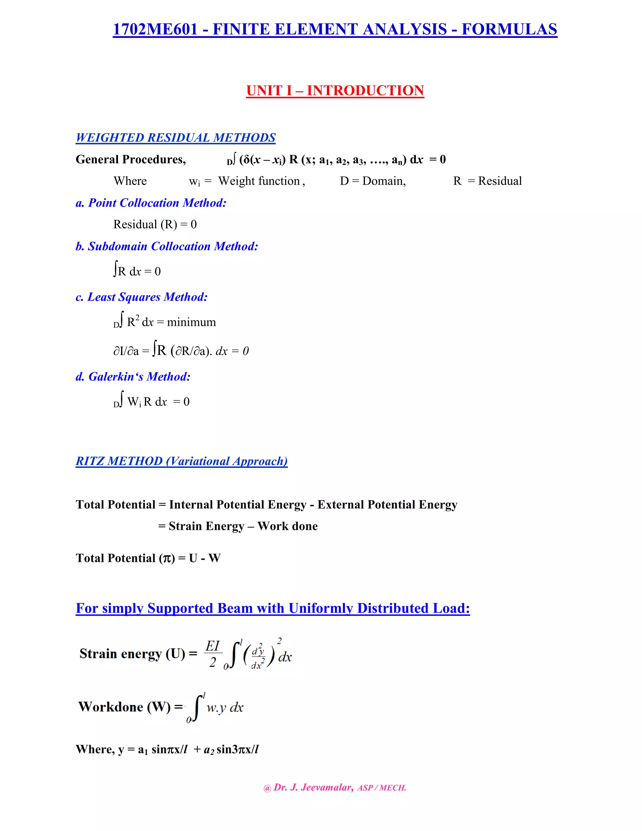
1) Weighted residual methods like point collocation, subdomain collocation, least squares, and Galerkin's method.
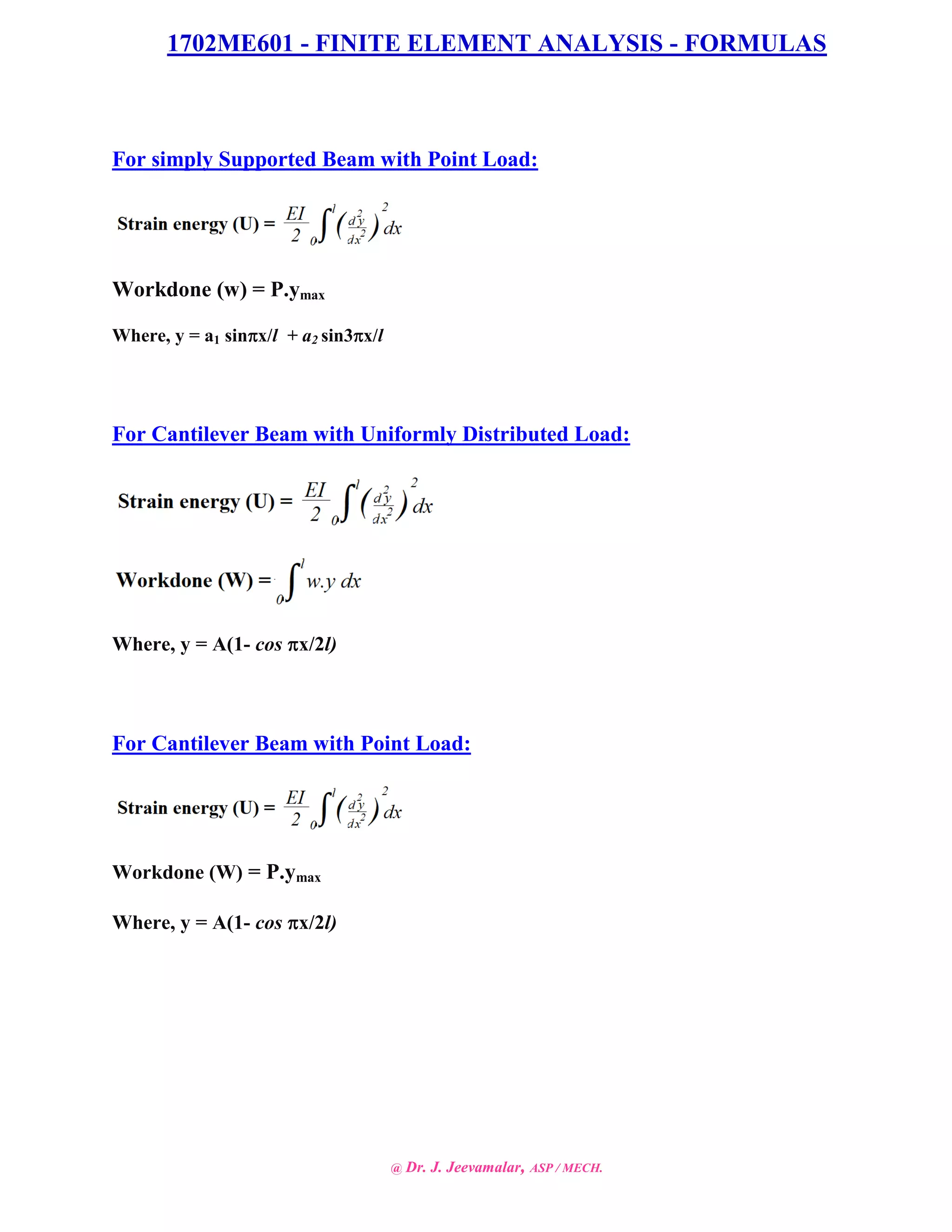
2) The Ritz method (variational approach) for calculating total potential energy of beams with different load cases.
3) Stress-strain and strain-displacement relationships, and formulas for calculating stiffness matrices and force vectors for bar, truss, beam and triangular elements.
4) Formulas for axisymmetric elements, heat transfer, isoparametric elements, and higher order elements.
Strain energy is a type of potential energy that is stored in a structural member as a result of elastic deformation. The external work done on such a member when it is deformed from its unstressed state is transformed into (and considered equal to the strain energy stored in it.
Applied Mathematics Multiple Integration by Mrs. Geetanjali P.Kale.pdfGeetanjaliRao6
In mathematics (specifically multivariable calculus), a Multiple Integral is a Definite Integral of a function of several real variables, for instance, f(x, y) or f(x, y, z). Integrals of a function of two variables over a region in (the real-number plane) are called Double Integrals, and integrals of a function of three variables over a region in (real-number 3D space) are called Triple Integrals. For multiple integrals of a single-variable function, see the Cauchy formula for repeated integration.
International Journal of Mathematics and Statistics Invention (IJMSI) inventionjournals
International Journal of Mathematics and Statistics Invention (IJMSI) is an international journal intended for professionals and researchers in all fields of computer science and electronics. IJMSI publishes research articles and reviews within the whole field Mathematics and Statistics, new teaching methods, assessment, validation and the impact of new technologies and it will continue to provide information on the latest trends and developments in this ever-expanding subject. The publications of papers are selected through double peer reviewed to ensure originality, relevance, and readability. The articles published in our journal can be accessed online.
The purpose of this work is to formulate and investigate a boundary integral method for the solution of the internal waves/Rayleigh-Taylor problem. This problem describes the evolution of the interface between two immiscible, inviscid, incompressible, irrotational fluids of different density in three dimensions. The motion of the interface and fluids is driven by the action of a gravity force, surface tension at the interface, elastic bending and/or a prescribed far-field pressure gradient. The interface is a generalized vortex sheet, and dipole density is interpreted as the (unnormalized) vortex sheet strength. Presence of the surface tension or elastic bending effects introduces high order derivatives into the evolution equations. This makes the considered problem stiff and the application of the standard explicit time-integration methods suffers strong time-step stability constraints.
The proposed numerical method employs a special interface parameterization that enables the use of an efficient implicit time-integration method via a small-scale decomposition. This approach allows one to capture the nonlinear growth of normal modes for the case of Rayleigh-Taylor instability with the heavier fluid on top.
Validation of the results is done by comparison of numeric solution to the analytic solution of the linearized problem for a short time. We check the energy and the interface mean height preservation. The developed model and numerical method can be efficiently applied to study the motion of internal waves for doubly periodic interfacial flows with surface tension and elastic bending stress at the interface.
All of material inside is un-licence, kindly use it for educational only but please do not to commercialize it.
Based on 'ilman nafi'an, hopefully this file beneficially for you.
Thank you.
We understand that you're a college student and finances can be tight. That's why we offer affordable pricing for our online statistics homework help. Your future is important to us, and we want to make sure you can achieve your degree without added financial stress. Seeking assistance with statistics homework should be simple and stress-free, and that's why we provide solutions starting from a reasonable price.
Visit statisticshomeworkhelper.com or email info@statisticshomeworkhelper.com. You can also call +1 (315) 557-6473 for assistance with Statistics Homework.
if you are struggling with your Multiple Linear Regression homework, do not hesitate to seek help from our statistics homework help experts. We are here to guide you through the process and ensure that you understand the concept and the steps involved in performing the analysis. Contact us today and let us help you ace your Multiple Linear Regression homework!
Visit statisticshomeworkhelper.com or email info@statisticshomeworkhelper.com. You can also call +1 (315) 557-6473 for assistance with Statistics Homework.
this is presentation on " skewed plate problem " which is related to advanced mechanic of material of subject.here explain about principle,method and approximation function with also steps wise for solving problem in Ritz method and discuss about the skewed plate problem. included conclusion and references.
Immunizing Image Classifiers Against Localized Adversary Attacksgerogepatton
This paper addresses the vulnerability of deep learning models, particularly convolutional neural networks
(CNN)s, to adversarial attacks and presents a proactive training technique designed to counter them. We
introduce a novel volumization algorithm, which transforms 2D images into 3D volumetric representations.
When combined with 3D convolution and deep curriculum learning optimization (CLO), itsignificantly improves
the immunity of models against localized universal attacks by up to 40%. We evaluate our proposed approach
using contemporary CNN architectures and the modified Canadian Institute for Advanced Research (CIFAR-10
and CIFAR-100) and ImageNet Large Scale Visual Recognition Challenge (ILSVRC12) datasets, showcasing
accuracy improvements over previous techniques. The results indicate that the combination of the volumetric
input and curriculum learning holds significant promise for mitigating adversarial attacks without necessitating
adversary training.
Hybrid optimization of pumped hydro system and solar- Engr. Abdul-Azeez.pdffxintegritypublishin
Advancements in technology unveil a myriad of electrical and electronic breakthroughs geared towards efficiently harnessing limited resources to meet human energy demands. The optimization of hybrid solar PV panels and pumped hydro energy supply systems plays a pivotal role in utilizing natural resources effectively. This initiative not only benefits humanity but also fosters environmental sustainability. The study investigated the design optimization of these hybrid systems, focusing on understanding solar radiation patterns, identifying geographical influences on solar radiation, formulating a mathematical model for system optimization, and determining the optimal configuration of PV panels and pumped hydro storage. Through a comparative analysis approach and eight weeks of data collection, the study addressed key research questions related to solar radiation patterns and optimal system design. The findings highlighted regions with heightened solar radiation levels, showcasing substantial potential for power generation and emphasizing the system's efficiency. Optimizing system design significantly boosted power generation, promoted renewable energy utilization, and enhanced energy storage capacity. The study underscored the benefits of optimizing hybrid solar PV panels and pumped hydro energy supply systems for sustainable energy usage. Optimizing the design of solar PV panels and pumped hydro energy supply systems as examined across diverse climatic conditions in a developing country, not only enhances power generation but also improves the integration of renewable energy sources and boosts energy storage capacities, particularly beneficial for less economically prosperous regions. Additionally, the study provides valuable insights for advancing energy research in economically viable areas. Recommendations included conducting site-specific assessments, utilizing advanced modeling tools, implementing regular maintenance protocols, and enhancing communication among system components.
Saudi Arabia stands as a titan in the global energy landscape, renowned for its abundant oil and gas resources. It's the largest exporter of petroleum and holds some of the world's most significant reserves. Let's delve into the top 10 oil and gas projects shaping Saudi Arabia's energy future in 2024.
Final project report on grocery store management system..pdfKamal Acharya
In today’s fast-changing business environment, it’s extremely important to be able to respond to client needs in the most effective and timely manner. If your customers wish to see your business online and have instant access to your products or services.
Online Grocery Store is an e-commerce website, which retails various grocery products. This project allows viewing various products available enables registered users to purchase desired products instantly using Paytm, UPI payment processor (Instant Pay) and also can place order by using Cash on Delivery (Pay Later) option. This project provides an easy access to Administrators and Managers to view orders placed using Pay Later and Instant Pay options.
In order to develop an e-commerce website, a number of Technologies must be studied and understood. These include multi-tiered architecture, server and client-side scripting techniques, implementation technologies, programming language (such as PHP, HTML, CSS, JavaScript) and MySQL relational databases. This is a project with the objective to develop a basic website where a consumer is provided with a shopping cart website and also to know about the technologies used to develop such a website.
This document will discuss each of the underlying technologies to create and implement an e- commerce website.
Sachpazis:Terzaghi Bearing Capacity Estimation in simple terms with Calculati...Dr.Costas Sachpazis
Terzaghi's soil bearing capacity theory, developed by Karl Terzaghi, is a fundamental principle in geotechnical engineering used to determine the bearing capacity of shallow foundations. This theory provides a method to calculate the ultimate bearing capacity of soil, which is the maximum load per unit area that the soil can support without undergoing shear failure. The Calculation HTML Code included.
6th International Conference on Machine Learning & Applications (CMLA 2024)ClaraZara1
6th International Conference on Machine Learning & Applications (CMLA 2024) will provide an excellent international forum for sharing knowledge and results in theory, methodology and applications of on Machine Learning & Applications.
6th International Conference on Machine Learning & Applications (CMLA 2024)
finite_element_analysis_formulas.pdf
1. 1702ME601 - FINITE ELEMENT ANALYSIS - FORMULAS
@ Dr. J. Jeevamalar, ASP / MECH.
UNIT I – INTRODUCTION
WEIGHTED RESIDUAL METHODS
General Procedures, D∫ (δ(x – xi) R (x; a1, a2, a3, …., an) dx = 0
Where wi = Weight function , D = Domain, R = Residual
a. Point Collocation Method:
Residual (R) = 0
b. Subdomain Collocation Method:
∫R dx = 0
c. Least Squares Method:
D∫ R2
dx = minimum
I/a = ∫R (R/a). dx = 0
d. Galerkin‘s Method:
D∫ Wi R dx = 0
RITZ METHOD (Variational Approach)
Total Potential = Internal Potential Energy - External Potential Energy
= Strain Energy – Work done
Total Potential () = U - W
For simply Supported Beam with Uniformly Distributed Load:
Where, y = a1 sinx/l + a2 sin3x/l
2. 1702ME601 - FINITE ELEMENT ANALYSIS - FORMULAS
@ Dr. J. Jeevamalar, ASP / MECH.
For simply Supported Beam with Point Load:
Workdone (w) = P.ymax
Where, y = a1 sinx/l + a2 sin3x/l
For Cantilever Beam with Uniformly Distributed Load:
Where, y = A(1- cos x/2l)
For Cantilever Beam with Point Load:
Workdone (W) = P.ymax
Where, y = A(1- cos x/2l)
3. 1702ME601 - FINITE ELEMENT ANALYSIS - FORMULAS
@ Dr. J. Jeevamalar, ASP / MECH.
UNIT II – ONE DIMENSIONAL (1D) ELEMENTS
01. Stress – Strain relationship,
Stress, ζ (N/mm 2
) = Young’s Modulus, E (N/mm 2
) x Strain, e
02. Strain – Displacement Relationship
Strain {e} = du / dx
03. Strain {e} = [B] {U}
Where, {e} = Strain Martix
[B] = Strain – Displacement Matrix
{U} = Degree of Freedom (Displacement)
04. Stress {ζ} = [E] {e} = [D] {e} = [D] [B] {u}
Where, [E] = [D] =Stress – Strain Matrix
05. General Equation for Stiffness Matrix, [K] = ∫ [B]T
[D] [B] dv
v
Where, [B] = Strain - Displacement relationship Matrix
[D] = Stress - Strain relationship Matrix
06. General Equation for Force Vector, {F} = [K] {U}
Where, {F} = Global Force Vector
[K] = Stiffness Matrix
{U} = Global Displacements
(i) 1D BAR ELEMENTS:
01. Stiffness Matrix for 1D Bar element, [K] = AE 1 -1
l -1 1
02. Force Vector for 2 noded 1D Bar element, F1 = AE 1 -1 u1
F2 l -1 1 u2
03. If self weight is considered, the Load / Force Vector, {F}E = ρ A l 1
2 1
where ρ = Density, N/mm3
4. 1702ME601 - FINITE ELEMENT ANALYSIS - FORMULAS
@ Dr. J. Jeevamalar, ASP / MECH.
(ii) 1D TRUSS ELEMENTS:
01. General Equation for Stiffness Matrix, [K] = Ae Le l2
lm -l2
-lm
lm m2 -lm -m2
le -l2
-lm l2
lm
-lm -m2
lm m2
02. Force vector for 2-noded Truss elements,
F1 Ae Le l2
lm -l2
-lm u1
F2 lm m2 -lm -m2
u2
F3 le -l2
-lm l2
lm u3
F4 -lm -m2
lm m2
u4
Where, l = Cos θ = x2 – x1 / le
m = Sin θ = y2 – y1 / le
Length of the element (le) = (x2 – x1)2
+ (y2 – y1)2
(iii) 1D BEAM ELEMENTS:
01. Force Vector for Two noded Beam Element
F1 Ee Ie 12 6L -12 6L d1
m1 = 6L 4L2
-6L 2L2
1
F2 L3
-12 -6L 12 -6L d2
m2 6L 2L2
-6L 4L2
2
02. Stiffness Matrix for Two noded Beam Element
[K] = Ee Ie 12 6L -12 6L
6L 4L2
-6L 2L2
L3
-12 -6L 12 -6L
6L 2L2
-6L 4L2
Where,
I = Moment of Inertia (mm4
)
L = Length of the Beam (mm)
5. 1702ME601 - FINITE ELEMENT ANALYSIS - FORMULAS
@ Dr. J. Jeevamalar, ASP / MECH.
UNIT III – TWO DIMENSIONAL (2D) ELEMENTS
01. Displacement Vector, U = u
v
02. General Equation for Stress & Strain, ζx ex
Stress, ζ = ζy Strain, e = ey
ηxy xy
Where, σx = Radial Stress ex = Radial Strain
σy = Longitudinal Stress ey = Longitudinal Strain
τxy = Shear Stress xy = Shear Strain
03. Body Force, F = Fx
Fy
04. Strain – Displacement Matrix, [B] = 1 q1 0 q2 0 q3 0
2A 0 r1 0 r2 0 r3
Where r1 q1 r2 q2 r3 q3
q1 = y2 – y3 ; r1 = x3 – x2
q2 = y3 – y1 ; r2 = x1 – x3
q3 = y1 – y2 ; r3 = x2 - x1 All co-ordinates are in mm
05. Stress – Strain Relationship Matrix, [D]
a. FOR PLANE STRESS PROBLEM,
E 1 µ 0
[D] = µ 1 0
(1 – µ2
) 0 0 1 - µ
2
b. FOR PLANE STRAIN PROBLEM,
E (1 – µ) µ 0
[D] = µ (1 - µ ) 0
(1 + µ) (1 – 2 µ) 0 0 1 - 2 µ
2
Where, µ = Poisson’s Ratio
E = Young’s Modulus
6. 1702ME601 - FINITE ELEMENT ANALYSIS - FORMULAS
@ Dr. J. Jeevamalar, ASP / MECH.
06. Stiffness Matrix for 2D element / CST Element, [K] = [B]T
[D] [B] A t
Where, A = Area of the triangular element, mm2
= 1 1 x1 y1
1 x2 y2
2 1 x3 y3
t = Thickness of the triangular (CST) element, mm
07. Maximum Normal Stress, ζ max = ζ1 = ζx + ζy + (ζx - ζy) 2
+ η2
xy
2 2
08. Minimum Normal Stress, ζ min = ζ2 = ζx + ζy - (ζx - ζy) 2
+ η2
xy
2 2
09. Principal angle, tan 2θP = 2 ηxy
ζx - ζy
10. Stress equation for Axisymmetric Element,
ζr Where, σr = Radial Stress
Stress {ζ} = ζθ σθ = Longitudinal Stress
ζz σz = Circumferential Stress
ηrz τrz = Shear Stress
er Where, er = Radial Stress
Strain, {e} = eθ eθ = Longitudinal Stress
ez ez = Circumferential Stress
γrz γrz = Shear Stress
11. Stiffness matrix for Two Dimensional Axisymmetric Problems,
[K] = 2 π r A [B] T
[D] [B]
Where, Co-ordinate r = r1 + r2 + r3 / 3 & z = z1 + z2 + z3 / 3
8. 1702ME601 - FINITE ELEMENT ANALYSIS - FORMULAS
@ Dr. J. Jeevamalar, ASP / MECH.
UNIT IV – HEAT TRANSFER APPLICATIONS
TEMPERATURE PROBLEMS FOR 1D ELEMENTS
01. Temperature Force {F} = E A ΔT -1
1
Where, E = young’s Modulus (N/mm2
)
A = Area of the Element (mm2
)
= Coefficient of thermal expansion (o
C)
ΔT = Temperature Difference (o
C)
02. Thermal stress {ζ} = E (du/dx) – E ΔT Where du / dx = u1 – u2 / l
TEMPERATURE PROBLEMS FOR 2D PROBLEMS ELEMENTS
01. Temperature Force, { θ } or { f } = [B]T
[D] {e0} t A
a. For Plane Stress Problems,
ΔT
Initial Strain {e0} = ΔT
0
b. For Plane Strain Problems,
ΔT
Initial Strain {e0} = (1 + ν) ΔT
0
TEMPERATURE PROBLEMS AXISYMMETRIC TRIANGULAR ELEMENTS
Temperature Effects:
For Axisymmetric Triangular elements, Temperature Force, { f }t = [B]T
[D] {e}t * 2 π r A
Where,
F1u
F1w ΔT
{ f }t = F2u Strain {e} = ΔT
F2w 0
F3u ΔT
F3w
9. 1702ME601 - FINITE ELEMENT ANALYSIS - FORMULAS
@ Dr. J. Jeevamalar, ASP / MECH.
HEAT TRANSFER PROBLEMS FOR 1D ELEMENTS:
a. General equation for Force Vector, {F} = [KC] {T}
b. Stiffness Matrix for 1D Heat conduction Element, [KC] = A k 1 -1
l -1 1
c. For Heat convection Problems,
A k / l 1 -1 + h A 0 0 T1 = h T A 0
-1 1 0 1 T2 1
Where, k = Thermal conductivity of element, W/mK
A = Area of the element, m2
l = Length of the element, mm
h = Heat transfer Coefficient, W/m2
K
T = fluid Temperature, K
T = Temperature, K
10. 1702ME601 - FINITE ELEMENT ANALYSIS - FORMULAS
@ Dr. J. Jeevamalar, ASP / MECH.
UNIT V – HIGHER ORDER AND ISOPARAMETRIC ELEMENTS
01. Shape Function for 4 Noded Rectangular Elements (Using Natural Co-Ordinate)
N1 = ¼ (1 – ε) (1 – η) N3 = ¼ (1 + ε) (1 + η)
N2 = ¼ (1 + ε) (1 – η) N4 = ¼ (1 - ε) (1 + η)
02. Displacement,
u = N1u1 + N2u2 + N3u3 + N4u4 & v = N1v1 + N2v2 + N3v3 + N4v4
u1
` v1
u2
u = u = N1 0 N2 0 N3 0 N4 0 v2
v 0 N1 0 N2 0 N3 0 N4 u3
v3
u4
v4
03. To find a point of P,
x = N1x1 + N2x 2 + N3 x3 + N4 x4 & y = N1 y1 + N2 y2 + N3 y3 + N4 y4
x1
` y 1
x2
u = x = N1 0 N2 0 N3 0 N4 0 y2
y 0 N1 0 N2 0 N3 0 N4 x3
y3
x4
y4
04. Jaccobian Matrix, [J] = ∂x / ∂ε ∂y / ∂ε
∂x / ∂η ∂y / ∂η
Where,
J11 = ¼ - (1 - η) x1 + (1 - η) x2 + (1 + η) x3 – (1 + η) x4
J12 = ¼ - (1 - η) y1 + (1 - η) y2 + (1 + η) y3 – (1 + η) y4
12. 1702ME601 - FINITE ELEMENT ANALYSIS - FORMULAS
@ Dr. J. Jeevamalar, ASP / MECH.
09. Element Force vector, {F} e = [N] T
Fx
Fy
Where , N is the shape function for 4 nodded Quadrilateral elements
10. Numerical Integration (Gaussian Quadrature)
Where wi = Weight function
F (xi) = values of function at pre determined points
No. of
points
Location, xi Corresponding weights, wi
1 x1 = 0.000… 2.000
2
x1 = + √1/3 = + 0.577350269189
x2 = - √1/3 = - 0.577350269189
1.0000
3
x1 = + √3/5 = + 0.774596669241
x3 = -√3/5 = - 0.774596669241
x2 = 0.0000
5/9 = 0.5555555555
5/9 = 0.5555555555
8/9 = 0.8888888888
4
x1 = + 0.8611363116
x4 = - 0.8611363116
x2 = + 0.3399810436
x3 = - 0.3399810436
0.3478548451
0.3478548451
0.6521451549
0.6521451549