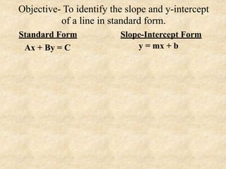
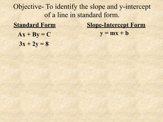
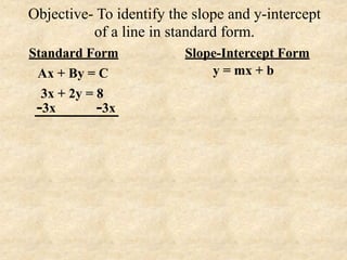
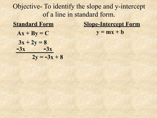
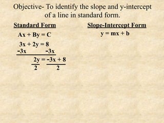
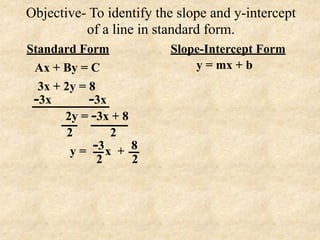
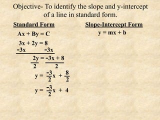
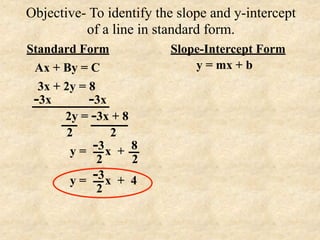
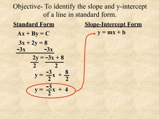
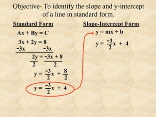
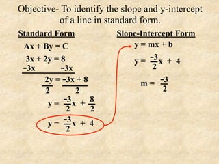
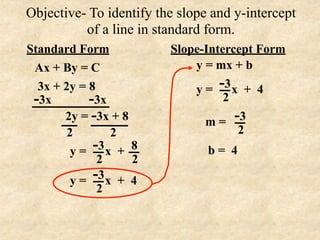
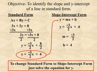
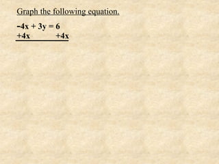
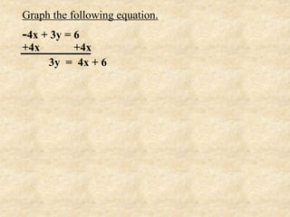
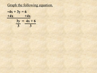
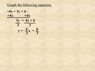
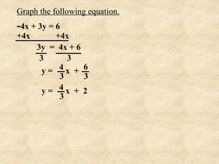
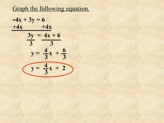
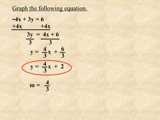
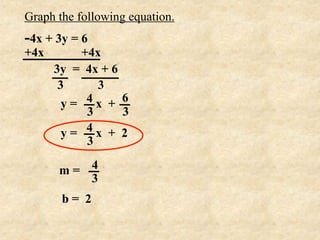
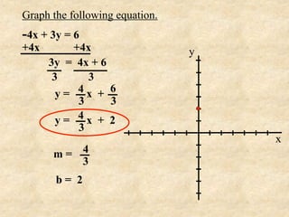
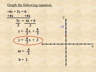
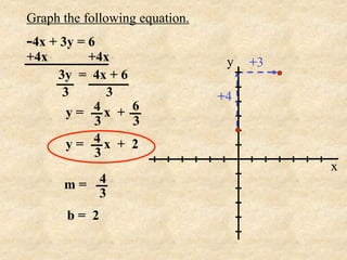
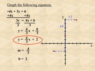
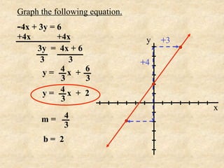
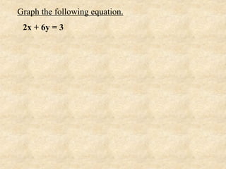
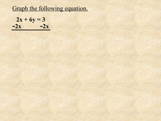
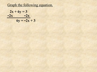
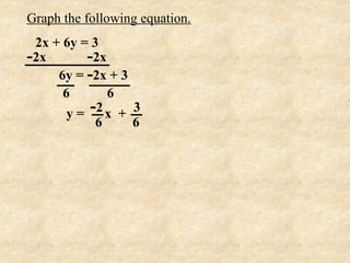
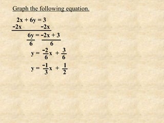
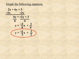
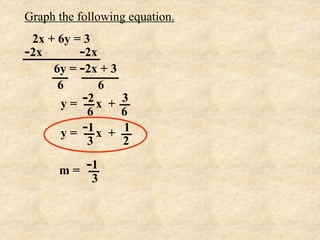
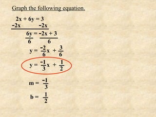
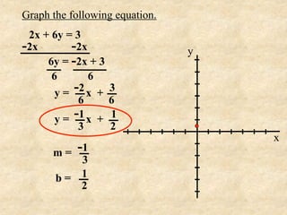
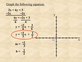
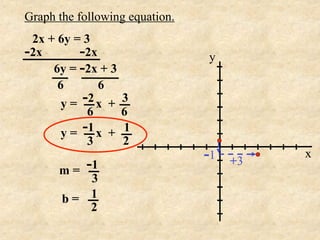
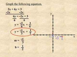
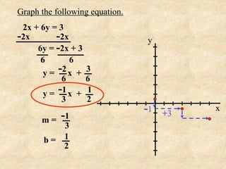
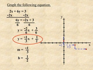
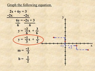
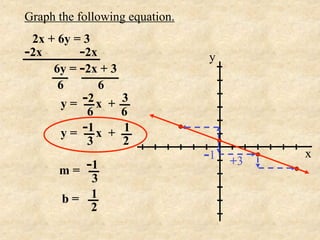
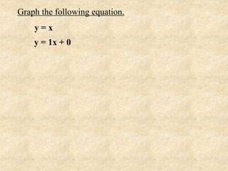
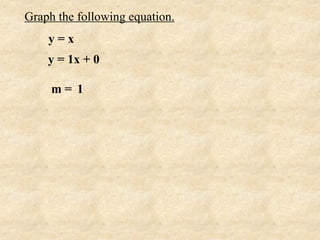
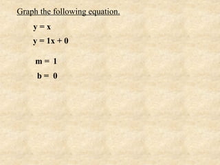
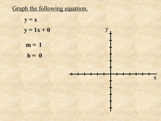
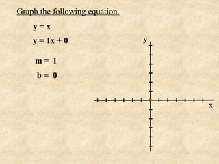
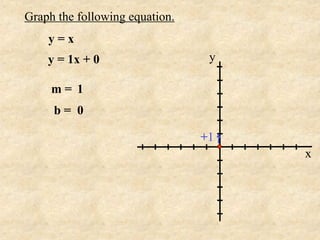
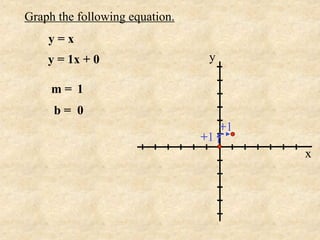
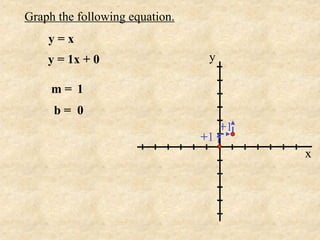
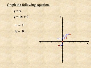
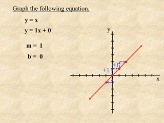
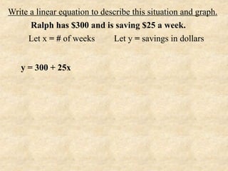
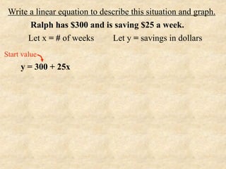
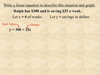
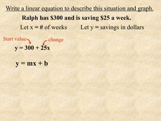
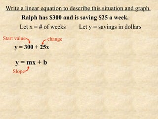
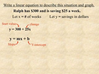
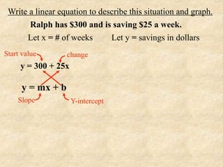
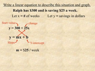
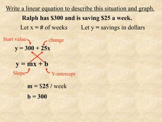
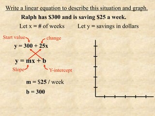
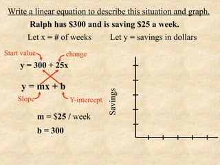
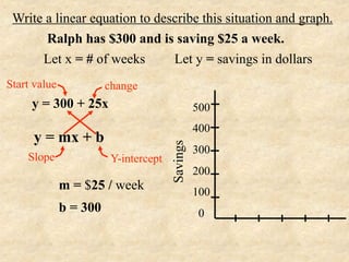
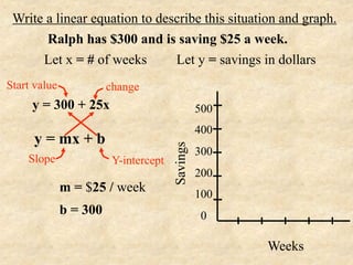
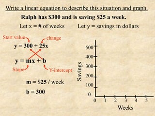
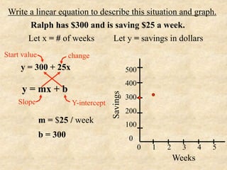
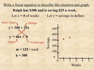
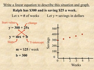
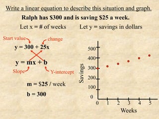
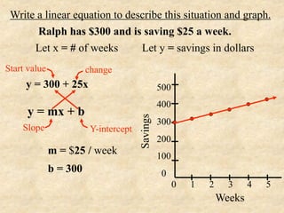
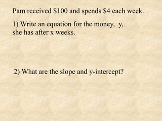
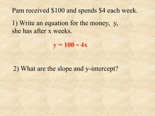
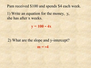
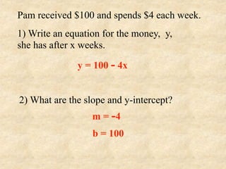
The document discusses how to identify the slope and y-intercept of a line given in standard form. It shows working through examples of changing lines from standard form (Ax + By = C) to slope-intercept form (y = mx + b). Through solving the equations for y, the slope (m) and y-intercept (b) can be determined. Graphing lines on a coordinate plane is also demonstrated.

1. Objective- To identify the slope and y-intercept
of a line in standard form.

2. Objective- To identify the slope and y-intercept
of a line in standard form.
Standard Form

3. Objective- To identify the slope and y-intercept
of a line in standard form.
Standard Form Slope-Intercept Form

4. Objective- To identify the slope and y-intercept
of a line in standard form.
Standard Form Slope-Intercept Form
Ax + By = C

5. Objective- To identify the slope and y-intercept
of a line in standard form.
Standard Form Slope-Intercept Form
Ax + By = C y = mx + b

6. Objective- To identify the slope and y-intercept
of a line in standard form.
Standard Form Slope-Intercept Form
Ax + By = C y = mx + b
3x + 2y = 8

7. Objective- To identify the slope and y-intercept
of a line in standard form.
Standard Form Slope-Intercept Form
Ax + By = C y = mx + b
3x + 2y = 8
-3x -3x

8. Objective- To identify the slope and y-intercept
of a line in standard form.
Standard Form Slope-Intercept Form
Ax + By = C y = mx + b
3x + 2y = 8
-3x -3x
2y = -3x + 8

9. Objective- To identify the slope and y-intercept
of a line in standard form.
Standard Form Slope-Intercept Form
Ax + By = C y = mx + b
3x + 2y = 8
-3x -3x
2y = -3x + 8
2 2

10. Objective- To identify the slope and y-intercept
of a line in standard form.
Standard Form Slope-Intercept Form
Ax + By = C y = mx + b
3x + 2y = 8
-3x -3x
2y = -3x + 8
2 2
y= -3 x + 8
2 2

11. Objective- To identify the slope and y-intercept
of a line in standard form.
Standard Form Slope-Intercept Form
Ax + By = C y = mx + b
3x + 2y = 8
-3x -3x
2y = -3x + 8
2 2
y= -3 x + 8
2 2
y = -3 x + 4
2

12. Objective- To identify the slope and y-intercept
of a line in standard form.
Standard Form Slope-Intercept Form
Ax + By = C y = mx + b
3x + 2y = 8
-3x -3x
2y = -3x + 8
2 2
y= -3 x + 8
2 2
y = -3 x + 4
2

13. Objective- To identify the slope and y-intercept
of a line in standard form.
Standard Form Slope-Intercept Form
Ax + By = C y = mx + b
3x + 2y = 8
-3x -3x
2y = -3x + 8
2 2
y= -3 x + 8
2 2
y = -3 x + 4
2

14. Objective- To identify the slope and y-intercept
of a line in standard form.
Standard Form Slope-Intercept Form
Ax + By = C y = mx + b
3x + 2y = 8 y = -3 x + 4
-3x -3x 2
2y = -3x + 8
2 2
y= -3 x + 8
2 2
y = -3 x + 4
2

15. Objective- To identify the slope and y-intercept
of a line in standard form.
Standard Form Slope-Intercept Form
Ax + By = C y = mx + b
3x + 2y = 8 y = -3 x + 4
-3x -3x 2
2y = -3x + 8 m= -3
2 2 2
y= -3 x + 8
2 2
y = -3 x + 4
2

16. Objective- To identify the slope and y-intercept
of a line in standard form.
Standard Form Slope-Intercept Form
Ax + By = C y = mx + b
3x + 2y = 8 y = -3 x + 4
-3x -3x 2
2y = -3x + 8 m= -3
2 2 2
y= -3 x + 8 b= 4
2 2
y = -3 x + 4
2

17. Objective- To identify the slope and y-intercept
of a line in standard form.
Standard Form Slope-Intercept Form
Ax + By = C y = mx + b
3x + 2y = 8 y = -3 x + 4
-3x -3x 2
2y = -3x + 8 m= -3
2 2 2
y= -3 x + 8 b= 4
2 2
y = -3 x + 4
2
To change Standard Form to Slope-Intercept Form
just solve the equation for y.

18. Objective- To identify the slope and y-intercept
of a line in standard form.
Standard Form Slope-Intercept Form
Ax + By = C y = mx + b
3x + 2y = 8 y = -3 x + 4
-3x -3x 2
2y = -3x + 8 m= -3
2 2 2
y= -3 x + 8 b= 4
2 2
y = -3 x + 4
2
To change Standard Form to Slope-Intercept Form
just solve the equation for y.

19. Graph the following equation.
-4x + 3y = 6

20. Graph the following equation.
-4x + 3y = 6
+4x +4x

21. Graph the following equation.
-4x + 3y = 6
+4x +4x
3y = 4x + 6

22. Graph the following equation.
-4x + 3y = 6
+4x +4x
3y = 4x + 6
3 3

23. Graph the following equation.
-4x + 3y = 6
+4x +4x
3y = 4x + 6
3 3
y= 4x + 6
3 3

24. Graph the following equation.
-4x + 3y = 6
+4x +4x
3y = 4x + 6
3 3
y= 4x + 6
3 3
y= 4x + 2
3

25. Graph the following equation.
-4x + 3y = 6
+4x +4x
3y = 4x + 6
3 3
y= 4x + 6
3 3
y= 4x + 2
3

26. Graph the following equation.
-4x + 3y = 6
+4x +4x
3y = 4x + 6
3 3
y= 4x + 6
3 3
y= 4x + 2
3
m= 4
3

27. Graph the following equation.
-4x + 3y = 6
+4x +4x
3y = 4x + 6
3 3
y= 4x + 6
3 3
y= 4x + 2
3
m= 4
3
b= 2

28. Graph the following equation.
-4x + 3y = 6
+4x +4x y
3y = 4x + 6
3 3
y= 4x + 6
3 3
y= 4x + 2
3
x
m= 4
3
b= 2

29. Graph the following equation.
-4x + 3y = 6
+4x +4x y
3y = 4x + 6
3 3
y= 4x + 6
3 3
y= 4x + 2
3
x
m= 4
3
b= 2

30. Graph the following equation.
-4x + 3y = 6
+4x +4x y
3y = 4x + 6
3 3 +4
y= 4x + 6
3 3
y= 4x + 2
3
x
m= 4
3
b= 2

31. Graph the following equation.
-4x + 3y = 6
+4x +4x y +3
3y = 4x + 6
3 3 +4
y= 4x + 6
3 3
y= 4x + 2
3
x
m= 4
3
b= 2

32. Graph the following equation.
-4x + 3y = 6
+4x +4x y +3
3y = 4x + 6
3 3 +4
y= 4x + 6
3 3
y= 4x + 2
3
x
m= 4
3
b= 2

33. Graph the following equation.
-4x + 3y = 6
+4x +4x y +3
3y = 4x + 6
3 3 +4
y= 4x + 6
3 3
y= 4x + 2
3
x
m= 4
3
b= 2

34. Graph the following equation.
-4x + 3y = 6
+4x +4x y +3
3y = 4x + 6
3 3 +4
y= 4x + 6
3 3
y= 4x + 2
3
x
m= 4
3
b= 2

35. Graph the following equation.
-4x + 3y = 6
+4x +4x y +3
3y = 4x + 6
3 3 +4
y= 4x + 6
3 3
y= 4x + 2
3
x
m= 4
3
b= 2

36. Graph the following equation.
2x + 6y = 3

37. Graph the following equation.
2x + 6y = 3
-2x -2x

38. Graph the following equation.
2x + 6y = 3
-2x -2x
6y = -2x + 3

39. Graph the following equation.
2x + 6y = 3
-2x -2x
6y = -2x + 3
6 6

40. Graph the following equation.
2x + 6y = 3
-2x -2x
6y = -2x + 3
6 6
y = -2 x + 3
6 6

41. Graph the following equation.
2x + 6y = 3
-2x -2x
6y = -2x + 3
6 6
y = -2 x + 3
6 6
y = -1 x + 1
3 2

42. Graph the following equation.
2x + 6y = 3
-2x -2x
6y = -2x + 3
6 6
y = -2 x + 3
6 6
y = -1 x + 1
3 2

43. Graph the following equation.
2x + 6y = 3
-2x -2x
6y = -2x + 3
6 6
y = -2 x + 3
6 6
y = -1 x + 1
3 2
m= -1
3

44. Graph the following equation.
2x + 6y = 3
-2x -2x
6y = -2x + 3
6 6
y = -2 x + 3
6 6
y = -1 x + 1
3 2
m= -1
3
b= 1
2

45. Graph the following equation.
2x + 6y = 3
-2x -2x y
6y = -2x + 3
6 6
y = -2 x + 3
6 6
y = -1 x + 1
3 2
x
m= -1
3
b= 1
2

46. Graph the following equation.
2x + 6y = 3
-2x -2x y
6y = -2x + 3
6 6
y = -2 x + 3
6 6
y = -1 x + 1
3 2
x
m= -1
3
b= 1
2

47. Graph the following equation.
2x + 6y = 3
-2x -2x y
6y = -2x + 3
6 6
y = -2 x + 3
6 6
y = -1 x + 1
3 2
-1 x
m= -1
3
b= 1
2

48. Graph the following equation.
2x + 6y = 3
-2x -2x y
6y = -2x + 3
6 6
y = -2 x + 3
6 6
y = -1 x + 1
3 2
-1 +3
x
m= -1
3
b= 1
2

49. Graph the following equation.
2x + 6y = 3
-2x -2x y
6y = -2x + 3
6 6
y = -2 x + 3
6 6
y = -1 x + 1
3 2
-1 +3
x
m= -1
3
b= 1
2

50. Graph the following equation.
2x + 6y = 3
-2x -2x y
6y = -2x + 3
6 6
y = -2 x + 3
6 6
y = -1 x + 1
3 2
-1 +3
x
m= -1
3
b= 1
2

51. Graph the following equation.
2x + 6y = 3
-2x -2x y
6y = -2x + 3
6 6
y = -2 x + 3
6 6
y = -1 x + 1
3 2
-1 +3
x
m= -1
3
b= 1
2

52. Graph the following equation.
2x + 6y = 3
-2x -2x y
6y = -2x + 3
6 6
y = -2 x + 3
6 6
y = -1 x + 1
3 2
-1 +3
x
m= -1
3
b= 1
2

53. Graph the following equation.
2x + 6y = 3
-2x -2x y
6y = -2x + 3
6 6
y = -2 x + 3
6 6
y = -1 x + 1
3 2
-1 +3
x
m= -1
3
b= 1
2

54. Graph the following equation.
2x + 6y = 3
-2x -2x y
6y = -2x + 3
6 6
y = -2 x + 3
6 6
y = -1 x + 1
3 2
-1 +3
x
m= -1
3
b= 1
2

55. Graph the following equation.
y=x

56. Graph the following equation.
y=x
y = 1x + 0

57. Graph the following equation.
y=x
y = 1x + 0
m= 1

58. Graph the following equation.
y=x
y = 1x + 0
m= 1
b= 0

59. Graph the following equation.
y=x
y = 1x + 0 y
m= 1
b= 0
x

60. Graph the following equation.
y=x
y = 1x + 0 y
m= 1
b= 0
x

61. Graph the following equation.
y=x
y = 1x + 0 y
m= 1
b= 0
+1
x

62. Graph the following equation.
y=x
y = 1x + 0 y
m= 1
b= 0
+1
+1
x

63. Graph the following equation.
y=x
y = 1x + 0 y
m= 1
b= 0
+1
+1
x

64. Graph the following equation.
y=x
y = 1x + 0 y
m= 1
b= 0
+1
+1
x

65. Graph the following equation.
y=x
y = 1x + 0 y
m= 1
b= 0
+1
+1
x

66. Graph the following equation.
y=x
y = 1x + 0 y
m= 1
b= 0
+1
+1
x

67. Graph the following equation.
y=x
y = 1x + 0 y
m= 1
b= 0
+1
+1
x

68. Graph the following equation.
y=x
y = 1x + 0 y
m= 1
b= 0
+1
+1
x

69. Write a linear equation to describe this situation and graph.
Ralph has $300 and is saving $25 a week.

70. Write a linear equation to describe this situation and graph.
Ralph has $300 and is saving $25 a week.
Let x = # of weeks

71. Write a linear equation to describe this situation and graph.
Ralph has $300 and is saving $25 a week.
Let x = # of weeks Let y = savings in dollars

72. Write a linear equation to describe this situation and graph.
Ralph has $300 and is saving $25 a week.
Let x = # of weeks Let y = savings in dollars
y = 300 + 25x

73. Write a linear equation to describe this situation and graph.
Ralph has $300 and is saving $25 a week.
Let x = # of weeks Let y = savings in dollars
Start value
y = 300 + 25x

74. Write a linear equation to describe this situation and graph.
Ralph has $300 and is saving $25 a week.
Let x = # of weeks Let y = savings in dollars
Start value change
y = 300 + 25x

75. Write a linear equation to describe this situation and graph.
Ralph has $300 and is saving $25 a week.
Let x = # of weeks Let y = savings in dollars
Start value change
y = 300 + 25x
y = mx + b

76. Write a linear equation to describe this situation and graph.
Ralph has $300 and is saving $25 a week.
Let x = # of weeks Let y = savings in dollars
Start value change
y = 300 + 25x
y = mx + b
Slope

77. Write a linear equation to describe this situation and graph.
Ralph has $300 and is saving $25 a week.
Let x = # of weeks Let y = savings in dollars
Start value change
y = 300 + 25x
y = mx + b
Slope Y-intercept

78. Write a linear equation to describe this situation and graph.
Ralph has $300 and is saving $25 a week.
Let x = # of weeks Let y = savings in dollars
Start value change
y = 300 + 25x
y = mx + b
Slope Y-intercept

79. Write a linear equation to describe this situation and graph.
Ralph has $300 and is saving $25 a week.
Let x = # of weeks Let y = savings in dollars
Start value change
y = 300 + 25x
y = mx + b
Slope Y-intercept

80. Write a linear equation to describe this situation and graph.
Ralph has $300 and is saving $25 a week.
Let x = # of weeks Let y = savings in dollars
Start value change
y = 300 + 25x
y = mx + b
Slope Y-intercept
m = $25 / week

81. Write a linear equation to describe this situation and graph.
Ralph has $300 and is saving $25 a week.
Let x = # of weeks Let y = savings in dollars
Start value change
y = 300 + 25x
y = mx + b
Slope Y-intercept
m = $25 / week
b = 300

82. Write a linear equation to describe this situation and graph.
Ralph has $300 and is saving $25 a week.
Let x = # of weeks Let y = savings in dollars
Start value change
y = 300 + 25x
y = mx + b
Slope Y-intercept
m = $25 / week
b = 300

83. Write a linear equation to describe this situation and graph.
Ralph has $300 and is saving $25 a week.
Let x = # of weeks Let y = savings in dollars
Start value change
y = 300 + 25x
y = mx + b
Savings
Slope Y-intercept
m = $25 / week
b = 300

84. Write a linear equation to describe this situation and graph.
Ralph has $300 and is saving $25 a week.
Let x = # of weeks Let y = savings in dollars
Start value change
y = 300 + 25x 500
400
y = mx + b
Savings
300
Slope Y-intercept
200
m = $25 / week 100
b = 300 0

85. Write a linear equation to describe this situation and graph.
Ralph has $300 and is saving $25 a week.
Let x = # of weeks Let y = savings in dollars
Start value change
y = 300 + 25x 500
400
y = mx + b
Savings
300
Slope Y-intercept
200
m = $25 / week 100
b = 300 0
Weeks

86. Write a linear equation to describe this situation and graph.
Ralph has $300 and is saving $25 a week.
Let x = # of weeks Let y = savings in dollars
Start value change
y = 300 + 25x 500
400
y = mx + b
Savings
300
Slope Y-intercept
200
m = $25 / week 100
b = 300 0
0 1 2 3 4 5
Weeks

87. Write a linear equation to describe this situation and graph.
Ralph has $300 and is saving $25 a week.
Let x = # of weeks Let y = savings in dollars
Start value change
y = 300 + 25x 500
400
y = mx + b
Savings
300
Slope Y-intercept
200
m = $25 / week 100
b = 300 0
0 1 2 3 4 5
Weeks

88. Write a linear equation to describe this situation and graph.
Ralph has $300 and is saving $25 a week.
Let x = # of weeks Let y = savings in dollars
Start value change
y = 300 + 25x 500
400
y = mx + b
Savings
300
Slope Y-intercept
200
m = $25 / week 100
b = 300 0
0 1 2 3 4 5
Weeks

89. Write a linear equation to describe this situation and graph.
Ralph has $300 and is saving $25 a week.
Let x = # of weeks Let y = savings in dollars
Start value change
y = 300 + 25x 500
400
y = mx + b
Savings
300
Slope Y-intercept
200
m = $25 / week 100
b = 300 0
0 1 2 3 4 5
Weeks

90. Write a linear equation to describe this situation and graph.
Ralph has $300 and is saving $25 a week.
Let x = # of weeks Let y = savings in dollars
Start value change
y = 300 + 25x 500
400
y = mx + b
Savings
300
Slope Y-intercept
200
m = $25 / week 100
b = 300 0
0 1 2 3 4 5
Weeks

91. Write a linear equation to describe this situation and graph.
Ralph has $300 and is saving $25 a week.
Let x = # of weeks Let y = savings in dollars
Start value change
y = 300 + 25x 500
400
y = mx + b
Savings
300
Slope Y-intercept
200
m = $25 / week 100
b = 300 0
0 1 2 3 4 5
Weeks

92. Write a linear equation to describe this situation and graph.
Ralph has $300 and is saving $25 a week.
Let x = # of weeks Let y = savings in dollars
Start value change
y = 300 + 25x 500
400
y = mx + b
Savings
300
Slope Y-intercept
200
m = $25 / week 100
b = 300 0
0 1 2 3 4 5
Weeks

93. Write a linear equation to describe this situation and graph.
Ralph has $300 and is saving $25 a week.
Let x = # of weeks Let y = savings in dollars
Start value change
y = 300 + 25x 500
400
y = mx + b
Savings
300
Slope Y-intercept
200
m = $25 / week 100
b = 300 0
0 1 2 3 4 5
Weeks

94. Write a linear equation to describe this situation and graph.
Ralph has $300 and is saving $25 a week.
Let x = # of weeks Let y = savings in dollars
Start value change
y = 300 + 25x 500
400
y = mx + b
Savings
300
Slope Y-intercept
200
m = $25 / week 100
b = 300 0
0 1 2 3 4 5
Weeks

95. Pam received $100 and spends $4 each week.

96. Pam received $100 and spends $4 each week.
1) Write an equation for the money, y,
she has after x weeks.
2) What are the slope and y-intercept?

97. Pam received $100 and spends $4 each week.
1) Write an equation for the money, y,
she has after x weeks.
y = 100 - 4x
2) What are the slope and y-intercept?

98. Pam received $100 and spends $4 each week.
1) Write an equation for the money, y,
she has after x weeks.
y = 100 - 4x
2) What are the slope and y-intercept?
m = -4

99. Pam received $100 and spends $4 each week.
1) Write an equation for the money, y,
she has after x weeks.
y = 100 - 4x
2) What are the slope and y-intercept?
m = -4
b = 100

100. Pam received $100 and spends $4 each week.
1) Write an equation for the money, y,
she has after x weeks.
y = 100 - 4x
2) What are the slope and y-intercept?
m = -4
b = 100