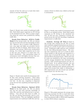
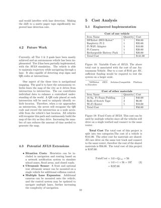
This document summarizes a capstone design project report for an Autonomous Vehicle Learning System (AVLS). The project involved designing an autonomous vehicle that can navigate a mock city using computer vision, networking, and route optimization algorithms. A software simulation was also created to model how the AVLS could optimize traffic flow on a large scale. The simulation showed that an optimal AVLS system without human traffic could improve average vehicle speed by 20% and reduce travel times by up to 66% compared to traditional traffic. The project demonstrated capabilities for autonomous vehicles to optimize traffic through decentralized data collection and routing.

1. Capstone Design Final Report
Robotics and Computer Vision
Autonomous Vehicle Learning System
[Robotics Team]
Authors:
Luke Miller
Robert Schultz
Rahul Tandon
Supervisor:
Professor Kristin Dana
Rutgers State University of New Jersey
Department of Electrical and Computer Engineering
May 8, 2016

2. 1 Introduction
The Autonomous Vehicle Learning System
(AVLS) enables evolutionary optimization of traf-
fic systems through individual vehicle data col-
lection. The goal of the AVLS is the design and
control of an autonomous vehicle, using network
communication, computer vision and route op-
timization. This concept can be scaled to con-
sumer sized vehicles, promoting a revolutionized
transportation system with no dependency upon
human based traffic indicators. On a small scale,
lane and sign detection enable the AVLS robot
to avoid obstacles and navigate an un-mapped
mock city testbed. As intersections are registered,
newly discovered paths between nodes are com-
municated to a centralized server which optimizes
routes over time. Vehicles will drive cyclically
between a set of destinations using paths selected
by a centralized server. This study demonstrates
important capabilities of autonomous travel as a
widespread form of transportation.
1.1 Problem Statement
Current traffic systems rely on visual indicators
to limit congestion and accidents. Humans are
error prone, and require signals to aid in naviga-
tion. Machines do not require visual instruction
and can make use of nearly instantaneous wireless
communication. Using computer vision, robotics
and machine learning, autonomous vehicles can be
realized that exceed the human capability of driv-
ing. This will reduce accident-related mortality,
optimize route navigation and limit overall traffic
congestion.
1.2 Major Components
The Autonomous Vehicle Learning System has
been divided into two subgroups with specific fo-
cuses on Robotic Design & Control and Computer
Vision. Components within the Robotics group
include: Hardware Design, Network Communica-
tion, and a Proportional Integral Derivative Drive
Controller. Components within the Computer Vi-
sion group include: Lane Detection, Stop Sign
Recognition and Intersection Identification., and
large-scale simulation.
Required Components:
• Four-wheel Drive Robotic Base
• Single Board Computer
• Wireless Networking Adapter
• Computer Vision Camera
• Test Bed Platform
• Isolated Wireless Communication Network
• Vehicle Data Processing Server
2 Methods / Objectives
Tier 1 - Primary Goals
Hardware Control The Tier 1 hardware goal of
AVLS is to design and build a small autonomous
vehicle capable of lane and traffic indicator de-
tection. The vehicle has independent drive trains
controlled by a four way H-Bridge motor con-
troller. Both rear wheels utilize rotary encoders
to track position. The Raspberry Pi connects to
a private and encrypted router which facilitates
communication with a local server.
Hardware Components:
• Single-board Computer: Raspberry Pi 2;
26 I/O pins programmable via C++ and
Python
• X-Media USB Wireless Adapter; 300 Mb/s
Network Communication
• Raspberry Pi Camera Module; 2592 x 1944
Resolution; 90fps
• Baron Four-wheel Drive Robotic Base; Two
Rotary Encoders
• D-Link Gigabit Wireless Router; WPA2
Network Encryption
• New Trent 10,000 mAh Backup Battery with
2A and 1A output
Noteworthy parameters to evaluate:
• Test-bed Materials
• Robotic Platform
Figure 1: This is the final robotic platform de-
signed by the AVLS robotics sub-team. The four
independently controlled motors proved to be crit-
ical for precise navigation.
The preliminary robotic implementation of
AVLS was heavily dependent on the modification
2

3. on an existing remote control car. While this ve-
hicle selection was cheaper for initial testing and
design, the robot proved to be inaccurate and un-
reliable in terms of speed and unintended drift.
Without an integrated Pulse Width Modulation
speed controller and variable degrees of turning,
it was nearly impossible to precisely navigate the
vehicle.
The final implementation, as seen in Figure
1 incorporates integrated PWM control, four-way
independent drive and rotary encoders. The speed
of the vehicle can be specified through an open
source library, and turning can be accurately con-
trolled by adjusting the ratio of left to right wheel
speeds.
Software Control The software priority in
tier 1 is to engineer a vehicle control utility. The
autonomous vehicle must smoothly stay within it’s
lane, stop at traffic indicators and consistently
perform turns at an intersection. Robotic soft-
ware control bridges raw computer vision data to
instruct hardware for test-bed navigation.
Smooth driving is dependent on the implemen-
tation of a Proportional Integral Derivative Con-
troller tuned to a specific operational environment.
The proportional term defines a proportional rate
at which the location of the robot must be ad-
justed after each each cycle. The integral term
addresses the accumulation of error over time in
a particular direction. This term eliminates the
buildup of offsets. The derivative term dictates
the rate at which error adjustments are made.
Derivative terms address the vehicle overshooting
a target trajectory. Though AVLS has both error
angle and error displacement as metrics for lane
deviation, the current PID only uses horizontal
displacement as an input argument for the con-
troller. After PID implementation, there was a
substantial decrease in the average angle error of
the vehicle over time. This indicates smoother er-
ror correction as opposed to a basic proportional
controller.
Noteworthy parameters to evaluate:
• Lighting Conditions
• PID Controller Parameters
• Robot Speed
Tier 2 - Secondary Goals
These goals have not yet been realized in
robotic form, but are discussed and analyzed
through a software simulation.
Scalability This project aims to demonstrate
the scalability of learning systems for Autonomous
Vehicles. The vehicles should be reproducible
with uniform components, and specifications. The
newly created vehicles will be immersed in an en-
vironment together, and will perform consistently
during nominal and off-nominal behavior. At this
stage, each vehicle will recognize another as a
generic obstacle, and basic maneuvers will be used
to avoid collision.
Noteworthy parameters to evaluate:
• Vehicle Count
Navigational Mapping In order to achieve
tier 2 secondary goals, navigational mapping is re-
quired for a stable system. This enables a vehicle
to detect its location within the environment with
relation to other vehicles or obstacles around it.
A local map is generated by each vehicle based on
landmarks at intersections, and each local map is
converged into a global map.
Noteworthy parameters to evaluate:
• Map Size
• Lane Count
• Road Distances
Tier 3 - Tertiary Goals
These goals have not yet been realized in
robotic form, but are discussed and analyzed
through a software simulation.
Communications Navigational mapping will
open possibilities into vehicle-vehicle communica-
tion. To implement this feature, cellular radios
will transmit individual vehicle data to a central-
ized location which distributes pertinent informa-
tion to each car. Alternatively, vehicles can com-
municate data through a peer-peer network and
bypass reliance on a central server. The route of
each vehicle will be calculated dynamically based
upon parameters collected from each car.
Noteworthy parameters to evaluate:
• Wireless Signal Band (WLAN, Bluetooth,
USRP)
• Communication Method (Server, Peer-to-
Peer)
Route Optimization Once a communication
network is established between vehicles, a func-
tional path will be found using depth or breadth
first search. The current global map and traffic
knowledge is used heuristically to develop an opti-
mal path between predefined destinations for the
vehicles. This route optimization happens in real-
time, allowing dynamic access for any vehicle dur-
ing run time. Random mutations in routes due to
3

4. traffic or obstacles can aid in the selection of more
optimal routes over time.
Noteworthy parameters to evaluate:
• Sort Algorithm of Indexed Paths
• Initial Path Algorithms
Software Simulation
Overview The AVLS simulation is a graph-
ical representation of how AVLS will operate on
a large scale. While autonomous vehicles (AVs)
explore an un-mapped city, they populate nodes
and edges of a directed graph. Individual findings
are concatenated with a unified global map on a
server. The server is responsible for aiding the AVs
in navigation. To process visuals, GraphStream
API is used to more easily facilitate analysis.
Algorithm As each vehicle seeks it’s own des-
tination, an A* searching algorithm is performed
on the server-side unified map to determine short-
est path for each car. The A* search algorithm is
a modified version of Dijkstra’s algorithm, which
creates a tree evaluating the weights of each edge.
A* was selected for its heuristic-based weights in
graph searching.
Simulation Design and Goal The goal of
this simulation is to monitor and evaluate traffic
flow under the AVLS system. While each vehicle
follows their most optimal route to predetermined
destinations, the length and condition of the pro-
cess can be evaluated systematically. Parameters
addressed are vehicle count, graph / route weight-
ing schemes, map design, as well as average traffic
speed and driving times.
Behavioral States The AVLS will operate in
3 states on a macroscopic level: a transient state,
transitioning state, and steady state. The behav-
ior of the system is modeled by state, with the
transient state initializing the system, transition-
ing state switching system modes, and steady state
modeling system behavior as time progresses.
Each of the behavioral states can be seen as the
simulation switches between conventional traffic,
AVLS with traffic indicators, and an ideal AVLS
implementation with no human-based traffic indi-
cators.
Transient State Behavior At the start of
the simulation, AVs do not have prior knowledge of
their environment. They drive locally and commu-
nicate their location to a centralized server, which
stores all pertinent information on the vehicles for
route navigation and traffic analysis. When in-
tersections are visited by multiple AVs, the server
connects the locations as nodes in a graph to prop-
erly analyze the city.
Figure 2: Graphing Algorithm Illustrated. This
demonstrates the mapping of a previously un-
known location. In part 4, the world is completely
mapped and an optimal path can be found be-
tween two nodes.
Transitioning Behavior Figure 2 contains
four major stages of the graphing algorithm for a
small town. First, vehicles map their local area as
they drive around. As vehicles arrive at already
discovered nodes, individual segments begin to
join together in a global map. After enough nodes
are found to link a given starting location to a
destination, the searching algorithm can be per-
formed while vehicles complete the map.
Driving Patterns The simulation contains
AVs that are programmed to drive to different
destinations following a certain parameter-based
driving mode. Route navigation is done based
upon the distance weights between each intersec-
tion; varying these weights results in noticeably
different behaviors in the AVs. In a deployed sys-
tem, these weights would need to be tuned to the
specific environment. Sample weights may or may
not include traffic depending on the mode of AVLS
implementation.
Steady State Behavior: Traditional Traf-
fic Mode This test mode serves as the control
group representative of current driving mecha-
nisms. The AVs are placed into a mock city with
no communication or traffic recognition. Driving
blindly into congestion, heavy traffic grows within
real-time minutes of simulation. This causes the
4

5. amount of time for each car to reach their desti-
nation to increase drastically.
Figure 3: Steady state model of traditional traffic
flow. Each black square represents an AV driving
in the simulated test bed. There is major conges-
tion along the central road, prohibitively halting
traffic flow.
Steady State Behavior: AVLS & Traffic
Mode In the second mode, the AVs are thrown
into the test bed with real-time knowledge of other
AVs. However, due to modern traffic infrastruc-
ture, stop signs and lights are prevalent factors
that slow the flow of vehicles. These factors cause
slowdown and prevent AVLS from synchronized
driving. As a result, light congestion can be seen
in this test case, however it is much more uni-
formly distributed. This intermediate phase of
autonomous travel will lightly decrease time nec-
essary for cars to reach their destinations.
Figure 4: Steady state model of autonomous traf-
fic flow with real-time heuristics. Each black
square represents an AV driving in the simulated
test bed. In this case, congestion is dispersed
across the test bed, equalizing and improving traf-
fic flow.
Steady State Behavior: Optimal AVLS
Mode In the third mode, the AVs are placed
into the test bed with real-time knowledge of
other AVs, and the road infrastructure is not pro-
hibitive. Cars will not slow down in traffic, as
the AVs are driving harmoniously, and in a syn-
chronized fashion. This case highlights significant
improvements over traditional traffic flow and rep-
resents a future in which every vehicle on the road
is autonomous.
Figure 5: Steady state model of autonomous traf-
fic flow in an optimal system. Each black square
represents an AV driving in the simulated test
bed. In this test case, congestion is greatly dis-
persed across the test bed, providing a significant
improvement to traffic flow.
Analysis: Average AV Time In figure 6,
the average time required for the AVs to reach
their randomly assigned destinations was shown to
decrease as a result of each mode of autonomous
travel. Traditional traffic patterns were modeled
for the first fifteen-thousand frames. The aver-
age time required for each car to reach its desti-
nation peaked at 100 seconds and remained at a
steady state of around 90 seconds. After an ad-
ditional fifteen-thousand frames, AVLS with traf-
fic mode was simulated in the same environment
and the average simulation time decreased to 60
seconds, a 33% overall improvement over the tra-
ditional mode. In an optimal situation, the cars
would not have to slow as a result of traffic. The
third mode exhibited peak optimal performance
around 30 seconds from origin to destination, a
50% improvement over the second case and 66%
improvement over the first case.
Figure 6: This graph represents the average simu-
lated time necessary for AVs to reach their desti-
nations. The line breaks denote a change in mode
from conventional traffic to AVLS with congestion,
to ideal AVLS without congestion.
5

6. Analysis: Average AV Speed In figure 7,
the average speed of the AVs was plotted versus
simulated time. The optimal speed of the AVs in
the simulation was set as 65mph, but as the city
is very populated, this goal cannot be reached. In
the first 800 frames of the simulation, the tradi-
tional traffic mode was evaluated, with about an
average of 15mph in the steady state. After the
800th frame, the AVLS navigation mode was ini-
tialized, and speed improved by 3 mph. The AVLS
system brought a 20% increase in average speed
for the vehicles. The third mode was not plotted,
as in an optimal system, all cars would be going
at the fastest speed of 65mph.
Figure 7: This line graph represents the average
simulated time required for AVs to reach their des-
tination. The line breaks denote a change in mode.
Analysis: Case Comparison Among the
three modes, the third mode had the highest per-
formance, while the second mode exhibited a sig-
nificant performance increase over current tradi-
tional traffic modes. This increase was between
12% and 17%. The AVLS demonstrates promis-
ing performance in cities that are not saturated
with vehicles, or when vehicles can be synchro-
nized with other AVs on the road.
Figure 8: This matrix of calculations displays
the performance increases between AVLS modes.
These figures include data from the ’transient’ por-
tion of the simulation as well as ’steady state’
3 Experimental Results
3.1 Speed Determination
Using proportional control, an experiment was
performed to determine an ideal speed with min-
imal error in both angle and displacement. As
expected, Trials depicted a 2.25 degree increase of
average error per Inch/Second increase in speed.
This is due largely to the networking delay induced
by streaming images and drive commands between
the server and vehicle. With a reduced speed, the
car is acting on more recent drive commands than
if the car were moving faster. In a full implemen-
tation, this would be resolved by an on-board com-
puter carrying the load of image processing.
Figure 9: Speed plotted against error rate in aver-
age horizontal displacement and angle. The graph
represents a linear increase in error angle for every
additional inch/second in speed. 2 inches/second
was chosen as the final robot speed as a compro-
mise between smooth driving and latency.
3.2 PID Coefficient Determination
u(t) = Kpe(t) + Ki
t
0
e(τ)dτ + Kd
de(t)
dt
(1)
An experiment was conducted to tune and
arithmetically determine the best coefficients for
a PID Controller. An over-head camera was uti-
lized to track the car as it traversed a straight
lane of six feet. In order to tune the PID parame-
ters, each were adjusted independently, and were
then adjusted simultaneously during the next set
of tests. For each set of coefficients, four trials
were conducted and a each resulting video was fed
into MATLAB to calculate the vehicle’s centroid.
Since the vehicle and test-bed color are distinct
shades, MATLAB can track the darkest area of
each frame and calculate it’s two-dimensional cen-
ter. The same vehicle centroid value was used for
each iteration of coefficients, and was utilized to
6

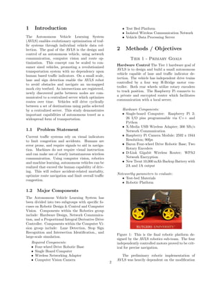
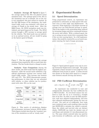
7. trace the vehicle across the frame.
Figure 10: Four trials were conducted using PID
values: P=.011, I=.0006,D=.001. The black line
represents the center of the lane, while colored
lines represent the vehicle’s deviation during each
trial.
In 3 out of 4 trials for the first parameter set,
the car was able to correct its path after deviation.
An average of the four trials is shown in Figure 11.
Figure 11: Four trials were conducted using PID
values: P=.011, I=.0006,D=.001. The black line
represents the center of the lane, while the red line
represents the average deviation of these four tri-
als.
This parameter set resulted in the AV closely
following the line with a max displacement of
around 30 pixels from the median, before return-
ing to the center. When scaled to fit every param-
eter set, as in 12, this set gives a clear and nearly
straight trajectory in relation to the center lane.
Figure 12: This trial represents the average vehi-
cle displacement for each parameter set in relation
to the center. Some parameter sets caused the car
to deviate a far greater distance from the center
of the lane than others. Looking at the averages
of all the PID variations, an optimal set of PID
values was selected.
Based off the results an equation for the PID
controller was determined. The coefficients used
were based off parameter set 1. Compared to the
other parameter sets , set 1 had the least devia-
tion over time and corrected its trajectory quickly
when off course.
Pn(e) = [.011]en + [.0006]
n
0
en + [.001]
den
dn
(2)
After PID implementation, the robot experi-
ences an average 2.93 degree error at the chosen
speed of 2in/sec. The result is a 73.12% decrease
in error from a simple proportional controller. Ad-
ditionally, the PID controller is used to counteract
driving errors that result from photo transfer la-
tency. This correction smoothing helps to prevent
the vehicle from over or under-turning based upon
asynchronous images.
3.3 Network Communication
The server and the Autonomous Vehicle must have
a pipeline through which to relay real time driv-
ing information. The server sends drive commands
based off processed images received from the car.
7

8. 3.3.1 Previous Implementation
Figure 13: The initial implementation of
AVLS’s Network Communication System was
quite lengthy. This was not an optimal process
because it takes too many steps for the car to re-
ceive a single drive command.
In the previously implement communication
system, a camera mounted on the car would cap-
ture and save a single photo at a time. A python
script running on the car reads the image and
transfers it over the network using the TCP proto-
col. Meanwhile, the server actively receives pack-
ets and writes them to a file. Single images are
transferred 1KB(1024 Bytes) at a time. Once an
entire image has been received, computer vision
is used to identify important features. The pro-
cessed drive command is relayed back to the car
which moves accordingly. This is a very lengthy
and convoluted process because the camera needs
to be initialized for each image.
The implementation in Figure 13 has many
points of failure that each induce latency. An
updated version of the process using an MJPEG
Stream is shown in Figure 14.
3.3.2 Current Implementation
Figure 14: The current implementation of AVLS’s
Network Communication System. This process re-
quires fewer steps compared to the original imple-
mentation.
In the current implementation a camera
mounted on the car starts an MJPEG stream
while a computer vision application on the server
processes and analyzes the frames in real time.
The server calculates angle and horizontal dis-
placement which is sent over the network to the
car’s PID controller.
Using the MJPEG stream significantly reduces
network transfer time. Images are read from a net-
work stream as opposed to being written to a file.
This helps to avoid memory leaks and decrease
time devoted to disk I/O.
The frame rate of the MJPEG stream was
adjusted with time to properly utilize the frame
buffer within the computer vision application. Ini-
tially, processing exhibited a 5 second delay during
initialization in order to clear the buffer of previ-
ously collected frames. Trials for frame rate deter-
mination are are discussed in the table below.
Image read configurations
Frame Rate Skipped Lag
24 FPS 0 Frames 5 seconds
24 FPS 1 Frames 4.5 seconds
24 FPS 2 Frames 4.2 seconds
24 FPS 3 Frames 3.9 seconds
24 FPS 4 Frames 3.4 seconds
24 FPS 5 Frames 2.6 seconds
12 FPS 0 Frames 3.7 seconds
12 FPS 1 Frames 3.1 seconds
12 FPS 2 Frames 2.5 seconds
12 FPS 3 Frames 1.5 seconds
12 FPS 4 Frames 1.4 seconds
12 FPS 5 Frames 1.4 seconds
6 FPS 0 Frames 3.3 seconds
6 FPS 1 Frames 2.2 seconds
6 FPS 2 Frames 1.7 seconds
6 FPS 3 Frames 1.3 seconds
Figure 15: Latency was measured using an ap-
proximation of the average time between an ac-
tion and it’s occurrence in the video feed. The
test examines a hand passing over the video feed.
A frame rate of 12 frames per second, with 3
frames being discarded at each loop, was chosen as
the optimal solution. Frames are skipped in order
to avoid an overload of Computer Vision buffer.
Any additional skipped frames would help reduce
lag but at a negative cost to driving accuracy.
8

9. Figure 16: These are example commands called by
the computer vision application to transfer the dis-
placement and angle to the car. The computer vi-
sion application uses a python script, passing two
arguments (displacement,angle), to transfer driv-
ing commands to the vehicle’s PID controller.
During testing, two network protocols were ex-
amined. Both Transmission Control Protocol and
User Datagram Protocol had benefits and draw-
backs for our specific implementation.
Transmission Control Protocol(TCP)
• Benefits: Error Checking.
• Drawbacks: Increased Latency.
User Datagram Protocol (UDP)
• Benefits: Fast Packet Transmission.
• Drawbacks: Potential Packet Loss.
Latency Table below compares the average
transfer time between network protocols: TCP
and UDP. TCP takes approximately 50 times as
long as UDP to send packets. Though the sam-
ple size is small, our preliminary testing indicates
UDP as a sufficient solution for AVLS network
communication. AVLS sends a data packet con-
taining an angle and a displacement value. A
test packet of 15 characters was used to conduct
the test. UDP took .1369 microseconds and TCP
took 7.05 microseconds to send the string message
of 15 characters. This experiment was performed
with packet sizes emulating driving commands,
but will be expanded to encompass image transfer
for a broader view on network communication.
Average Transfer Time
Network Protocol Average Time(s)
TCP 7.0532E-06
UDP 1.36971E-05
Figure 17: TCP v. UDP Latency (in seconds)
This chart shows the average time it takes to send
a data packet over TCP/UDP network Protocol.
Error The TCP network protocol checks for
dropped packets via verification from packet re-
cipients. UDP does not have this fail safe in place
and will occasionally lose packets. Packet loss is
highly detrimental in a real-time reasoning system
in which missing information could result in dam-
age of components.
4 Discussion
4.1 Challenges
The most significant problem with a remote com-
puter vision guiding controller has been the no-
ticeable latency between capturing frames from
the robot and asserting drive commands. When
tested in isolation, Python-based MJPEG stream-
ing over HTTP results in a noticeable but work-
able latency of around 200ms on average. The
primary contribution to this latency is line detec-
tion processing from the camera. This latency is
compensated using a tuned PID controller.
The initial selection of a robotic base proved
to be error prone. Due to manufacturing com-
plications, a misalignment existed between the
front wheels. This resulted in significant devi-
ation from a directed course. Despite attempts
to programmatically compensate for this drift,
experimentation indicated that deviation varied
greatly between multiple necessary driving oper-
ations. A new, more precise, robotic base was
chosen.
The simulation currently relies on data contri-
bution from individual vehicles within the system
and does not implement any learning algorithms
to optimize routes. The current method, referred
to as evolutionary optimization, utilizes random
paths for all the AVs, in order to best understand
the testbed, and optimize traffic flow. A chal-
lenge has been to employ system-wide learning
algorithms that unites the AVLS robot with the
software simulation.
The construction of a test environment has
been a developmental bottleneck that kept us from
properly testing network communication, driving
speed and PID coefficients. A uniform environ-
ment in which to perform repeatable tests is cru-
cial to determining success. The challenge was se-
lecting appropriate yet cost efficient materials and
a location for this test environment. Black elec-
trical tape lanes proved to be extremely reflective
9

10. and would interfere with lane detection. Making
the shift to a matte paper tape significantly im-
proved lane detection rate.
4.2 Future Work
Currently, all Tier 1 & 2 goals have been mostly
achieved and an autonomous vehicle has been im-
plemented. Tier 3 has been partially implemented,
with the AVLS simulation. The vehicle is able
to maintain trajectory while navigating through a
lane. It also capable of detecting stop signs and
QR codes at intersections.
One aspect of the these tiers is navigational
mapping. The goal is to have the autonomous ve-
hicles learn the map of the city as it drives from
intersection to intersection. The car contributes
individual data to enhance a centralized under-
standing of the world. A QR code placed at each
intersection will be used to uniquely identify ve-
hicle location. Therefore, when a car approaches
an intersection, the server will recognize the QR
code and record the intersection as a node acces-
sible from the vehicle’s last location. All vehicles
will recognize this path and continuously build the
map of the city as they drive. Increasing the num-
ber of cars reduces the amount of time needed to
generate the map.
4.3 Potential AVLS Extensions
• Situation Costs: Heuristics can be in-
cluded in navigation and routing based on
a network notification system to simulate
school zones, flood areas, and closed roads.
• Ultrasonic Sensor: A front and optional
rear ultrasonic sensor can be mounted on a
single vehicle for additional collision control.
• Multiple Lane Expansion: Additional
cameras can be mounted onto the vehicle,
and the control system may be updated to
navigate multiple lanes, further increasing
the complexity of navigation.
5 Cost Analysis
5.1 Engineered Implementation
Cost of one vehicle
Item Name Quantity Cost
DFRobot 4WD Robota
1 $56.00
Raspberry Pi 2 1 $35.00
Pi WiFi Adapter 1 $10.00
Pi Camera 1 $20.00
Rechargeable Battery Pack 1 $20.00
Total Cost $141.00
Figure 18: Variable Costs of AVLS. The above
total cost is associated with the cost of one Au-
tonomous Vehicle. Due to a cost of $141 per AV,
sufficient funding would be required to test the
system on a larger scale.
aDFRobot 4WD Arduino-Compatible Platform
w/Encoders
Cost of other materials
Item Name Quantity Cost
16 Sq. Ft Foam Padding 2 $40.00
Rolls of Scotch Tape 2 $6.00
Wi-Fi Router 1 $10.00
Total Cost $56.00
Figure 19: Fixed Costs of AVLS. This cost can be
used by multiple vehicles since all the vehicles will
drive on a single testbed and connect to the same
router.
Total Cost The total cost of this project is
split into two categories.The cost of a vehicle is
$141.00. The other cost for materials are shared.
All cars drive on the same test track and connect
to the same router, therefore the cost of the shared
materials is $56.00. The total cost of this project
is $197.00:
TotalCost = 141 ∗ QCar + 56
= 141 ∗ 1 + 56 = 197
= $197.00
(3)
10

11. 5.2 Commercial Implementation
In a commercial AVLS development scenario, a
test bed environment is not necessary to construct.
The car will house its own computer vision proces-
sor and will not need to offload real time calcula-
tions. Real cars drive at greater speeds so it is
essential to have a higher quality camera with im-
proved frame rate and resolution. The computer
vision should take advantage of a Graphics Pro-
cessing Unit for higher frame throughput. Poor
resolution images or skipped frames can lead to in-
correct commands which can be dangerous to the
passengers. Multiple infrared sensors are also nec-
essary in order to detect objects around the car,
so the car can make the appropriate movement to
avoid them.
The commercial implementation would also re-
quire a higher bandwidth communication network
in order to relay map and location information to
a centralized server.
Estimated cost
Item Name Quantity Cost
High speed camera 1 $250.00
NVIDIA GeForce 750 1 $100.00
Raspberry Pi 2 1 $35.00
Router 1 $200.00
IFARED Sensor 8 $800
Library licensing 1 Unknown
Total $1285+
Unknown
Figure 20: This represents estimates for the cost
of a real world implementation. These estimates
do not include the price of the car itself.
For safety purposes it is recommended to house
2 infrared sensors on each side of the car as well as
2 on the back and front. This is useful for detect-
ing objects next to the car that may in the blind
spot of a human driver. The sensors in the back
and front can aid in the avoidance of front and
rear collisions.
A graphics card like the NVIDIA GeForce 750
is a GPU used mainly on consumer desktops. It
has more power than the typical raspberry pi and
helps reduce latency during processing. The prices
shown above are subject to change as the quality
or quantity of the items are modified. For exam-
ple adding multiple cameras to provide a greater
range of view can increase the price depending on
the camera quality.
11

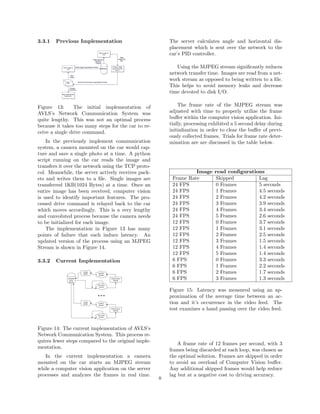
12. 6 Current Trends
Traditional automatic vehicle theory relies heav-
ily on probabilistic and stochastic analysis [5].
Although the scope of most research deviates into
advanced control systems, the basis for vehicle de-
sign relies on optical and gyroscopic sensors much
like the AVLS.
Companies like Google and Tesla are attempt-
ing to create a mass market standard for the
autonomous vehicle platform. Their vision is to
replace the human element in driving within our
lifetime. Many automotive manufacturers have
joined in to bring a small level of autonomy to their
current commercial lineup. New vehicle models
often feature self parking systems and guidance
auto pilots to keep their car in lane. This trend
began with automatic braking and has advanced
to commercial vehicles being summoned from a
remote location for use.
Kettering University One existing solution
of an autonomous vehicle was developed by stu-
dents at Kettering University.
The authors focus on how autonomous cars
would interact with each other while driving. This
alludes to a future where autonomous vehicles are
common place on the roads and humans are un-
necessary in the travel equation. When all vehicles
are autonomous, an individual unit will know its
particular position when compared to other au-
tonomous cars. Autonomous vehicles will be able
to relay this information to each other in order
to optimize traffic and avoid collision.[3] This is
similar to the goal of AVLS. In the future, stop
signs or street lights may not be required as an
autonomous vehicle will relay its information to
other autonomous vehicles and navigate accord-
ingly.
In order to reduce the on-board processing
done by the car, the students developed an exter-
nal Master Station. This master-slave relationship
reduces latency, decreases the number of compu-
tations done on the vehicle microprocessor, and
allows the implementation to be extended to mul-
tiple cars. [3] AVLS also uses an external server
to reduce load on Raspberry Pi. However, AVLS
in its current stage has only one master while
the students at Kettering University elected for a
one to one correlation between vehicles and offline
processing units. This may result in an enhanced
level of security and guaranteed, prioritized pro-
cessing time. [3]
AVLS uses a single camera to capture the
vehicle’s view and the server processes this infor-
mation and gives back an angle and displacement
value. The students’ implementation employs a
wide variety of sensors including a gyroscope, ac-
celerometer, compass and speed encoder to deter-
mine angular and linear position of the car. An IR
range sensor is also added so the car can avoid ob-
stacles it encounters. IR works more efficiently at
small distances which is practical for chaotic city
driving. [3]. The Master Station has an myRIO
real-time FPGA board which takes in local co-
ordinates and formulates the position of the car
in global coordinates.[3] Using this information
and a position sensor the car knows its relative
position in relation to the global coordinate plane.
Unlike AVLS, this implementation relies more on
sensor data rather than the camera feed, to drive
the car autonomously.
In a large scale setting the wireless commu-
nication must have an efficient range. AVLS is
using a local router where the car and server con-
nect. Similarly, the students used a Digi Xbee
Wireless module which gives a range of 300 feet
[3]. Having a greater range allows for a larger
test environment. This implementation also uses
a different protocol to transfer data between the
server and car. AVLS currently uses UDP network
protocol and will in the future use TCP protocol
since it is more reliable. The students used a
serial UART protocol with RTS/CTS handshake
for wireless communication because it reduces the
number of frame collisions that occur in the hid-
den node problem.[3] The hidden node problem
occurs when a particular node can see the host
node but not the nodes around it. This way a
car can communicate locality to other cars in the
system. This can be used to eliminate the need
for stop signs or street lights.
Google Self Driving Car On a larger scale,
Google is using similar methods to develop an au-
tonomous car system to transport passengers to
select destinations. This approach is a reevalua-
tion of conventional transportation systems with
an emphasis on automaticity. With a fleet of au-
tonomous vehicles individuals will not require per-
sonal vehicles and the number of cars on the road
will significantly decrease. Unlike AVLS which
relies on a camera for computer vision, Google
12

13. uses a single 64 beam laser to generate a three-
dimensional map of the car’s surroundings. This
rendering is cross-referenced with Google’s pro-
prietary high resolution world maps to increase
accuracy of the image. The downside of this ap-
proach is that the autonomous vehicles, while
highly accurate, require their environment to be
pre-mapped by another fleet of Google mapping
cars. The vehicle is equipped with four radars, for
long range object detection, a windshield mounted
camera, for traffic lights, a GPS, wheel encoders
and an inertial measurement unit. The culmina-
tion of these sensors provided the vehicle with a
contextual understanding of its environment and
allow it to detect anomalies even at far distances.
Google has been testing these Self Driving Cars
in Bay Area cities, with an supervisory human
driver on board. Although these tests have been
mostly successful, Google cars have been expe-
riencing accidents as a result of being unable to
predict the actions of human drivers. In an world
of entirely autonomous vehicles that communicate
their intentions, this would not be an issue. [2]
Dedicated Short Range Communication
Much like AVLS, DaimlerChrysler has taken a new
approach to autonomous travel through vehicle-
vehicle or vehicle-infrastructure communication.
DSCR piggy backs on IEEE 802.11a at 5.8GHz
with custom protocol modifications. Signals are
intended to be broadcast from each vehicle and re-
ceived by other near-by cars. This provides the ve-
hicle with an ”extended information horizon” that
allows the driver to be aware of situations that
may not yet be visible. Preliminary DSRC im-
plementations examine human operated vehicles
relaying critical safety information to surrounding
cars, in an attempt to reduce accident fatalities.
One proposed example is ”Traffic Signal Violation
Warning” which would notify an operator if their
vehicle is expected to enter an intersection on a
red light. This direct application of DSRC would
address nearly 2,300 yearly fatalities in the US.
One concern expressed with the DSCR is the pos-
sibility of overwhelming a driver with information,
ultimately distracting them from the road. The
research group has focused on the security and
scalability of their design. When receiving over
the air information from other vehicles that dic-
tates your car’s behavior, it is important to verify
that the data is coming from a legitimate source.
A primary concern of this method is the hijacking
of autonomous vehicles or the phishing of drivers
remotely through spoofed packets. Though the
primary directive of DSRC is to increase safety
of navigating road ways, DSCR could be used for
traffic advisory, electronic tolling, and updates to
digital maps. [1]
Cloud Computing for Robots Cloud com-
puting is becoming a cornerstone in a variety of in-
dustries from consumer applications to large-scale
mathematical processing. Companies like Amazon
and Google offer other businesses virtual computer
services hosted at off-site locations. In addition to
data security and redundancy, these shares of com-
putational power allow small and large companies
alike to exceed their own local processing ability at
a cheaper cost. This concept can be applied to the
case of artificial intelligence processing. In order
for artificial intelligence to become an integrated
part of a consumer’s daily life, access to powerful
computers must be cost effective and scalable to
any degree. Companies use cloud computing to
reduce the financial burden of purchasing expen-
sive computers that will be obsolete in a number
of years. This solution simultaneously addresses
the issue of off-site and redundancy backups of in-
formation. Businesses are only required to pay a
monthly or yearly fee to access hosted virtual ma-
chines for its employees.[4]
As electronics get smaller, they tend to rely
less on local processing power and more on of-
floading calculation. This trend also applies to
mass market robotics. The addition of powerful
computers and graphics cards can heavily inflate
the cost and weight of a robot, making them hard
to manufacture on a large scale. Cloud comput-
ing allows robots to become smaller while main-
taining access to increasingly powerful computing
resources. Much like AVLS, cloud computing en-
ables robots to instantaneously access information
from other units while contributing to a collective
of information.[4]
Cloud computing does have some drawbacks.
Slow communication speeds will hinder robotic
functionality, meaning that robots require redun-
dant high speed communication mechanisms. If
a robot were to lose connection to the host pro-
cessor, safety features must ensure graceful fail-
ure, or local computation must temporarily dic-
tate actions.[4]
The architecture for cloud robotics is broken
up into two levels: machine-to-cloud(M2C) and
machine-to-machine(M2M). M2C allows robots to
utilize the processing power of cloud based com-
puters for computation. M2M enables robots
to work synchronously in a collaborative effort
13

14. thus creating an ad-hoc cloud. This encour-
ages rapid information sharing and results in
the increased performance of many computational
units. [4] RobotEarth, an implementation of
cloud-computation, aims to bring these features
to a wide variety of robots. RobotEarth features
plug and play architecture which allows for new
features or nodes to be added without redesign-
ing the system.[4] RobotEarth uses the DAvinCi
framework, a software utility, that provides ac-
cess to parallel and scalable computing. A large
environment of service robots can take advan-
tage of the parallelism and scalability to increase
efficiency and means of communication between
them. RobotEarth uses the Robot Operating sys-
tem (ROS) to facilitate communication with the
DAvinCi server and the other robots. A Hadoop
Distributed File System (HDFS) connected to the
DAvinCi server is used to process complex compu-
tations requested by a robot. The DAvinCi server
acts as the master node and handles processing
and computation when robots do not have enough
resources. [4]
Businesses have used cloud computing to scale
their infrastructure quickly and efficiently. In or-
der for robots to become a part of our daily lives,
they need to take advantage of cloud computing
in order to maintain a cheap and efficient system.
References
[1] Vehicle communication. IEEE Pervasive Com-
puting October-December, 1536-1268, 2006.
[2] Erico Guizzo. How google’s self-driving car
works. IEEE Spectrum Online, October, 18,
2011.
[3] Dwarkesh Iyengar and Diane L Peters. De-
velopment of a miniaturized autonomous vehi-
cle: Modification of a 1: 18 scale rc car for
autonomous operation. In ASME 2015 Dy-
namic Systems and Control Conference, pages
V003T50A008–V003T50A008. American Soci-
ety of Mechanical Engineers, 2015.
[4] D Lorencik and Peter Sincak. Cloud robotics:
Current trends and possible use as a service. In
Applied Machine Intelligence and Informatics
(SAMI), 2013 IEEE 11th International Sym-
posium on, pages 85–88. IEEE, 2013.
[5] Cem ¨Unsal, Pushkin Kachroo, and John S Bay.
Multiple stochastic learning automata for ve-
hicle path control in an automated highway
system. Systems, Man and Cybernetics, Part
A: Systems and Humans, IEEE Transactions
on, 29(1):120–128, 1999.
14