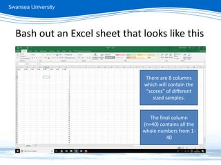
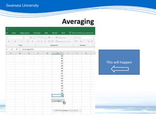
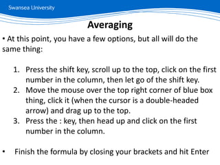
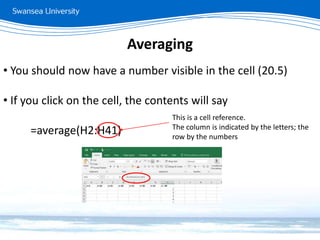
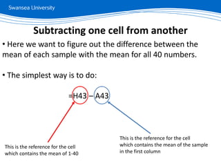
This document provides instructions for using simple formulae in Excel to calculate averages and differences between averages. It describes how to: 1. Enter an "=average()" formula in a cell to automatically calculate the average of a column of numbers. 2. Copy the average formula across multiple columns to calculate the average for each sample size. 3. Subtract one cell containing an overall average from another cell containing a sample average to determine the difference between the two averages. The goal is to use these basic Excel functions and cell references to analyze sample data and answer questions on an exercise sheet. Proper saving of the Excel file is also emphasized for continued use later.

1. Using simple formulae in Excel
David Playfoot
Swansea University

2. Bash out an Excel sheet that looks like this
There are 8 columns
which will contain the
“scores” of different
sized samples.
The final column
(n=40) contains all the
whole numbers from 1-
40

3. Averaging
• We will want to know the mean score for the sample in each
column.
• Excel will figure it out for you
• Select a cell (a box) after the end of the numbers 1-40
• I usually leave a few blank spaces for reasons that
will become apparent later in the module.

4. Averaging
• In your selected cell write
=average(
But do not hit Enter yet
• The = sign tells Excel that this is a formula it needs to work
on and not just information it needs to store.

5. Averaging
• In your selected cell write
=average(
But do not hit Enter yet
• Click on the last number in the column

6. Averaging
This will happen

7. • At this point, you have a few options, but all will do the
same thing:
1. Press the shift key, scroll up to the top, click on the first
number in the column, then let go of the shift key.
2. Move the mouse over the top right corner of blue box
thing, click it (when the cursor is a double-headed
arrow) and drag up to the top.
3. Press the : key, then head up and click on the first
number in the column.
• Finish the formula by closing your brackets and hit Enter
Averaging

8. Averaging
• You should now have a number visible in the cell (20.5)
• If you click on the cell, the contents will say
=average(H2:H41)
This is a cell reference.
The column is indicated by the letters; the
row by the numbers

9. • You should now have a number visible in the cell (20.5)
• Now copy your formula across the other 7 columns you’re
going to use. Keep it in the same row. The first 7 rows will
have “#DIV/0!” in because Excel doesn’t have any numbers to
use yet.
•Fill in your numbers according to the instructions in the
exercises file.
• Note: Excel will ignore any blank cell when it does the
average
Averaging

10. • Here we want to figure out the difference between the
mean of each sample with the mean for all 40 numbers.
• The simplest way is to do:
=H43 – A43
Subtracting one cell from another
This is the reference for the cell
which contains the mean of 1-40
This is the reference for the cell
which contains the mean of the sample
in the first column

11. • You should be able to use these skills to answer the
questions on your exercise sheet for section 1
• IT IS IMPORTANT THAT YOU SAVE THE EXCEL FILE ALONG –
WE WILL BE USING IT AGAIN IN A FEW WEEKS.
Simple formulae in Excel