Download to read offline
![DESCRIPTIVE STATISTICS USING R PROGRAMMING ALONG
WITH THE DEMONSTRATION
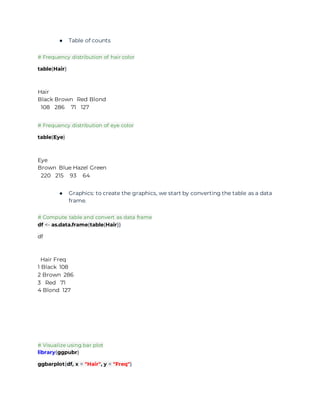
Frequency tables
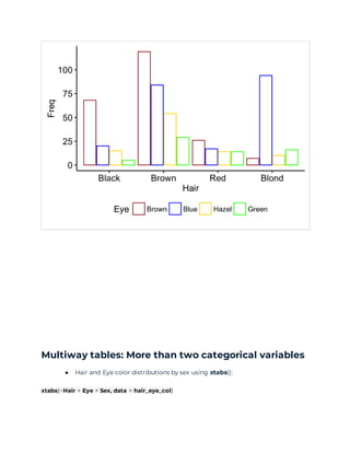
A frequency table (or contingency table) is used to describe categorical variables. It
contains the counts at each combination of factor levels.
R function to generate tables: table()
Create some data
Distribution of hair and eye color by sex of 592 students:
# Hair/eye color data
df <- as.data.frame(HairEyeColor)
hair_eye_col <- df[rep(row.names(df), df$Freq), 1:3]
rownames(hair_eye_col) <- 1:nrow(hair_eye_col)
head(hair_eye_col)
Hair Eye Sex
1 Black Brown Male
2 Black Brown Male
3 Black Brown Male
4 Black Brown Male
5 Black Brown Male
6 Black Brown Male
# hair/eye variables
Hair <- hair_eye_col$Hair
Eye <- hair_eye_col$Eye
Simple frequency distribution: one categorical
variable](https://image.slidesharecdn.com/example-2summerizationnotesfordescriptivestatisticsusingr-201105082316/85/Example-2-summerization-notes-for-descriptive-statistics-using-r-1-320.jpg)
![DESCRIPTIVE STATISTICS USING R PROGRAMMING ALONG
WITH THE DEMONSTRATION
Frequency tables
A frequency table (or contingency table) is used to describe categorical variables. It
contains the counts at each combination of factor levels.
R function to generate tables: table()
Create some data
Distribution of hair and eye color by sex of 592 students:
# Hair/eye color data
df <- as.data.frame(HairEyeColor)
hair_eye_col <- df[rep(row.names(df), df$Freq), 1:3]
rownames(hair_eye_col) <- 1:nrow(hair_eye_col)
head(hair_eye_col)
Hair Eye Sex
1 Black Brown Male
2 Black Brown Male
3 Black Brown Male
4 Black Brown Male
5 Black Brown Male
6 Black Brown Male
# hair/eye variables
Hair <- hair_eye_col$Hair
Eye <- hair_eye_col$Eye
Simple frequency distribution: one categorical
variable](https://image.slidesharecdn.com/example-2summerizationnotesfordescriptivestatisticsusingr-201105082316/75/Example-2-summerization-notes-for-descriptive-statistics-using-r-1-2048.jpg)
![, , Sex = Male
Eye
Hair Brown Blue Hazel Green
Black 32 11 10 3
Brown 53 50 25 15
Red 10 10 7 7
Blond 3 30 5 8
, , Sex = Female
Eye
Hair Brown Blue Hazel Green
Black 36 9 5 2
Brown 66 34 29 14
Red 16 7 7 7
Blond 4 64 5 8
● You can also use the function ftable() [for flat contingency tables]. It returns a
nice output compared to xtabs() when you have more than two variables:
ftable(Sex + Hair ~ Eye, data = hair_eye_col)
Sex Male Female
Hair Black Brown Red Blond Black Brown Red Blond
Eye
Brown 32 53 10 3 36 66 16 4
Blue 11 50 10 30 9 34 7 64
Hazel 10 25 7 5 5 29 7 5
Green 3 15 7 8 2 14 7 8
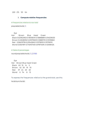
Compute table margins and relative frequency
Table margins correspond to the sums of counts along rows or columns of the table.
Relative frequencies express table entries as proportions of table margins (i.e., row or
column totals).](https://image.slidesharecdn.com/example-2summerizationnotesfordescriptivestatisticsusingr-201105082316/85/Example-2-summerization-notes-for-descriptive-statistics-using-r-7-320.jpg)

This document describes how to generate frequency tables and distributions in R to summarize categorical data. It discusses: 1. Creating simple frequency tables using the table() function to show counts of one or two categorical variables. 2. Generating two-way contingency tables using table() or xtabs() to examine relationships between two categorical variables. 3. Computing table margins with margin.table() and relative frequencies with prop.table() or converting tables to percentages.


![제 23회 보아즈(BOAZ) 빅데이터 컨퍼런스 - [MBOAX] : ABSA를 활용한 소비자 반응 분석 기반 운영 효율화 대시보드 설계](https://cdn.slidesharecdn.com/ss_thumbnails/3-1boaz23rdconferencemboax-260203102709-9d519923-thumbnail.jpg?width=640&height=640&fit=bounds)

![7.__Developing_a_Research_Proposal[1].pptx](https://cdn.slidesharecdn.com/ss_thumbnails/7-260131073037-df92dd7d-thumbnail.jpg?width=640&height=640&fit=bounds)


![Hacking-Uncovered-How-People-Get-Hacked-and-How-to-Stay-Safe[1].pptx](https://cdn.slidesharecdn.com/ss_thumbnails/hacking-uncovered-how-people-get-hacked-and-how-to-stay-safe1-260130170011-4883a9c7-thumbnail.jpg?width=640&height=640&fit=bounds)


