Downloaded 243 times


![Solving for the Estimated Gamma Function
• Select a series of strikes, Ki , and quantities, θi, to create a portfolio of
puts and calls.
• To estimate the gamma function we need to choose the amount of
options for each strike, θi , so as to minimize the distance between the
estimated gamma function and the true gamma function.
• Estimated gamma function equals:
N M
− Γ( P ) =
ˆ
∑Max( P − K , 0) ×θ + ∑Max( K
i =1
i i
i =1
i − P,0 ) ×θi
• Choose the optimal quantities by minimizing the sum of the squared
errors between the true and estimated gamma function over a set of Q
prices. 2
∑ [Γ( P ) − Γ( P )]
Q
min ˆ j j
θ
j =1
Hess Energy · 2010 All Rights Reserved
21](https://image.slidesharecdn.com/eucimay2011ericmeerdink-130308075947-phpapp01/75/Modeling-and-Hedging-the-Risk-in-Retail-Load-Contracts-21-2048.jpg)
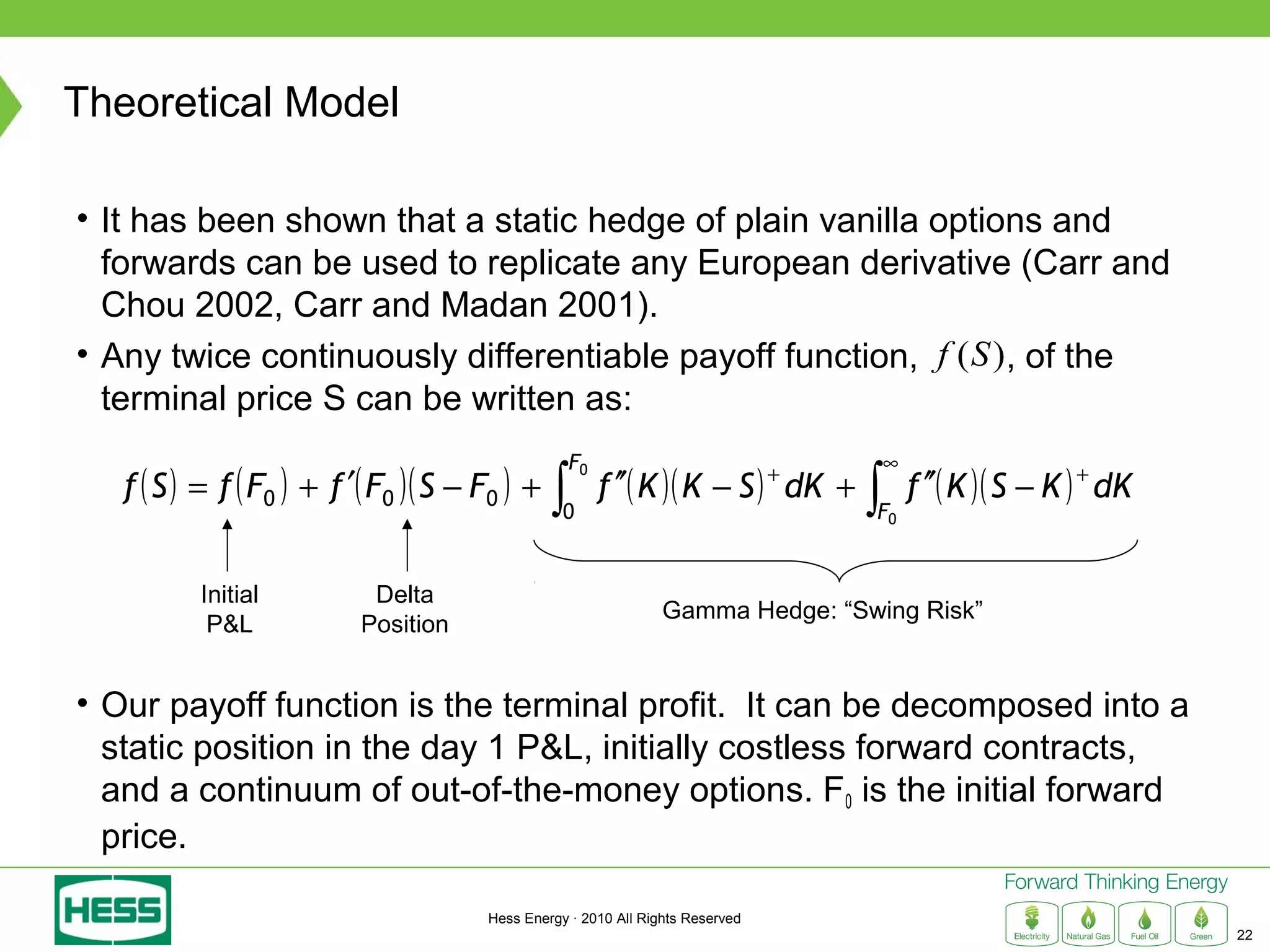
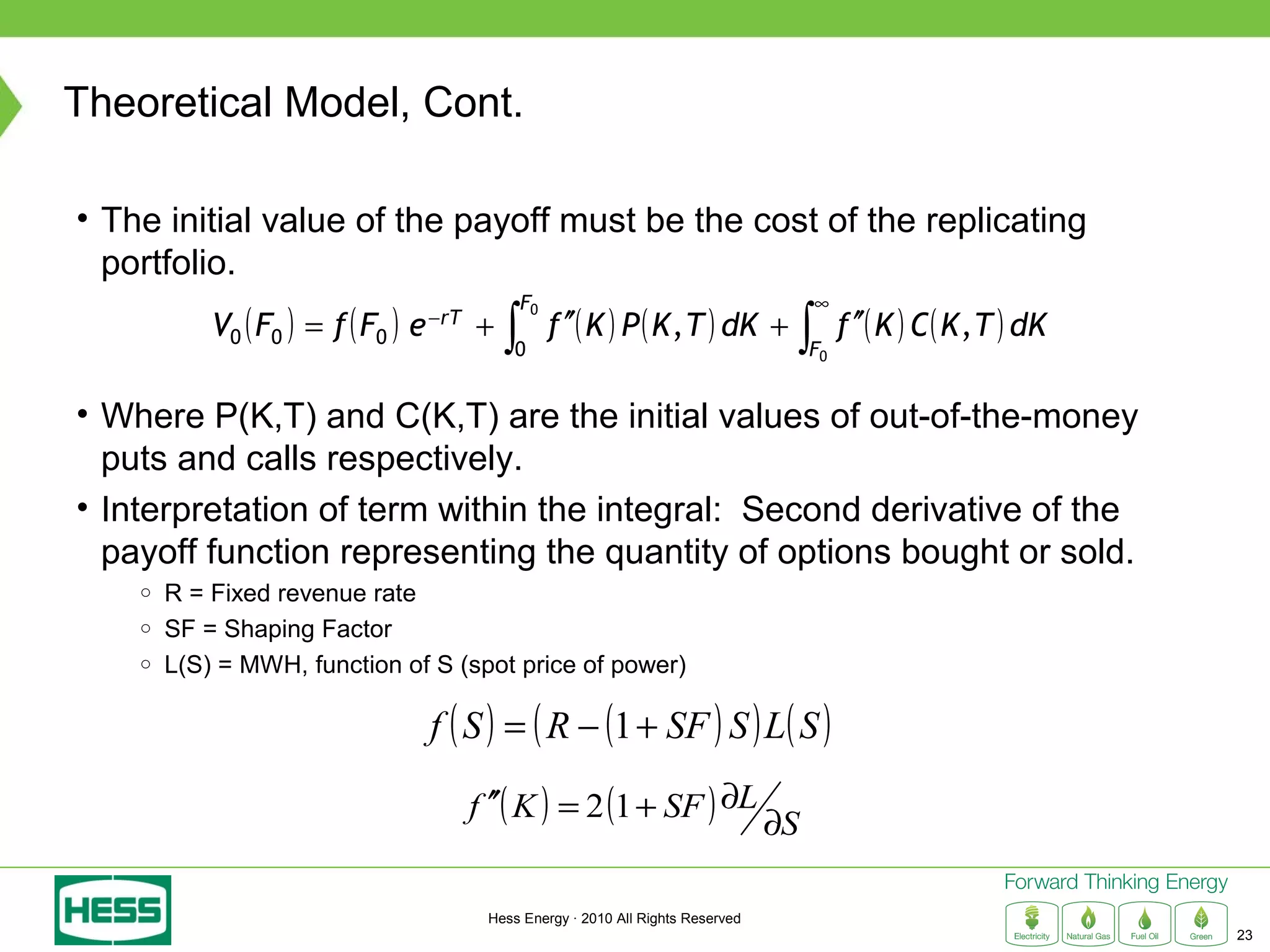
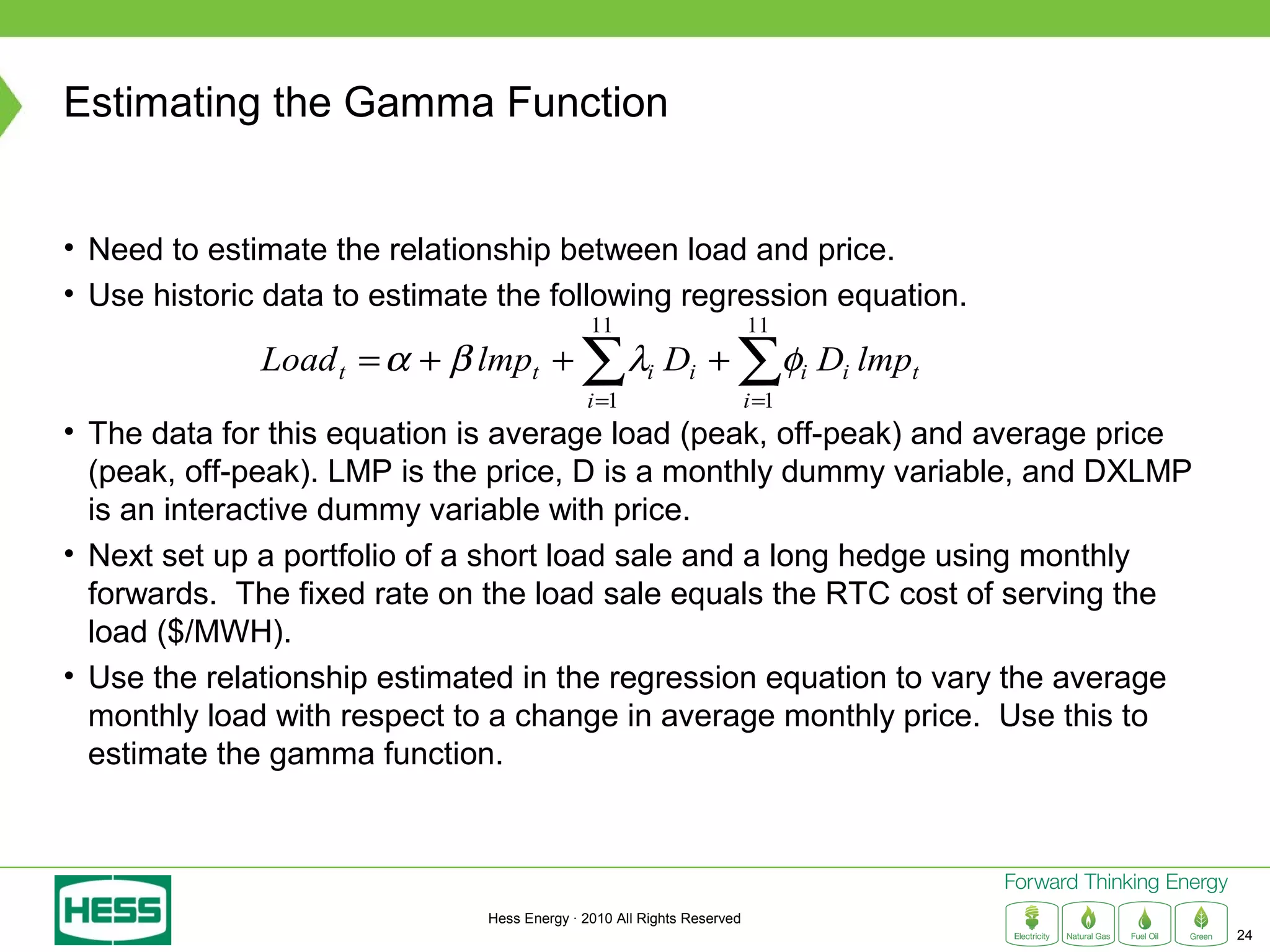
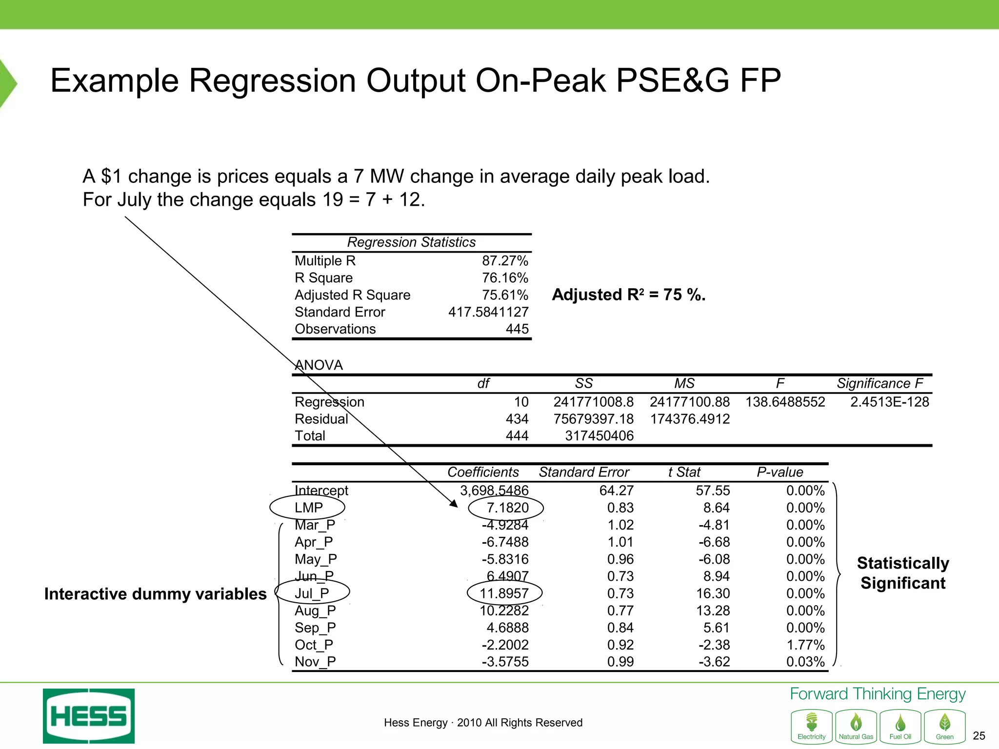
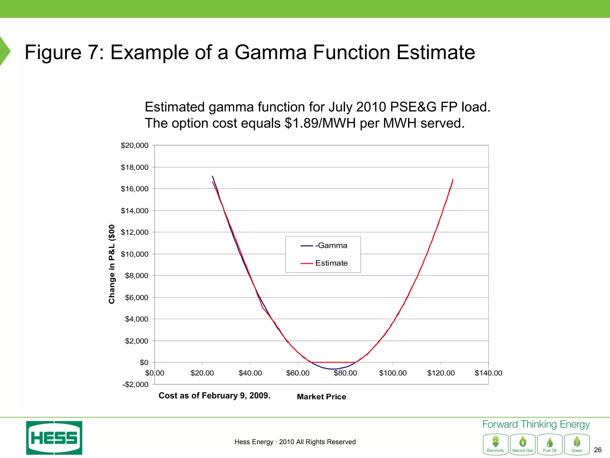
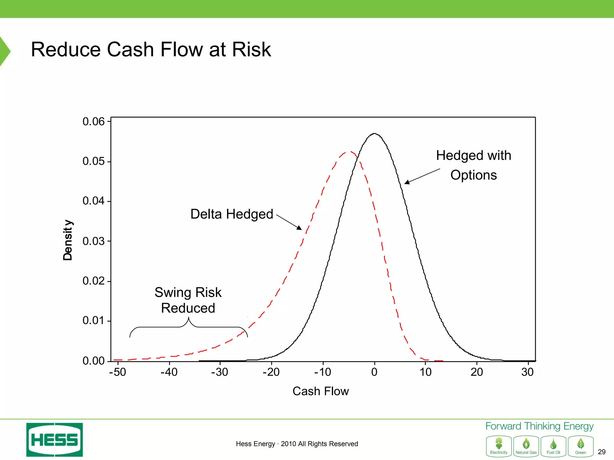
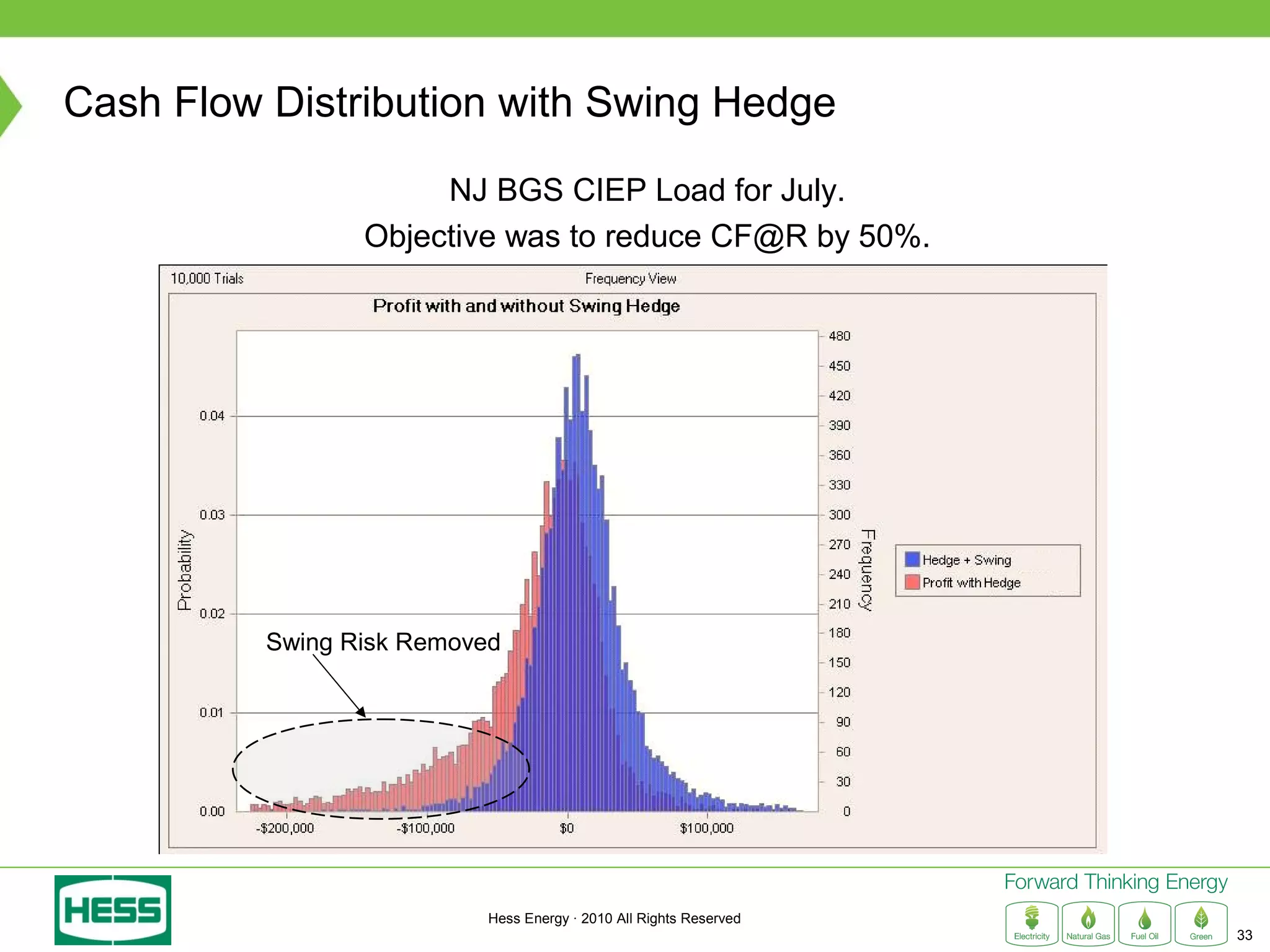
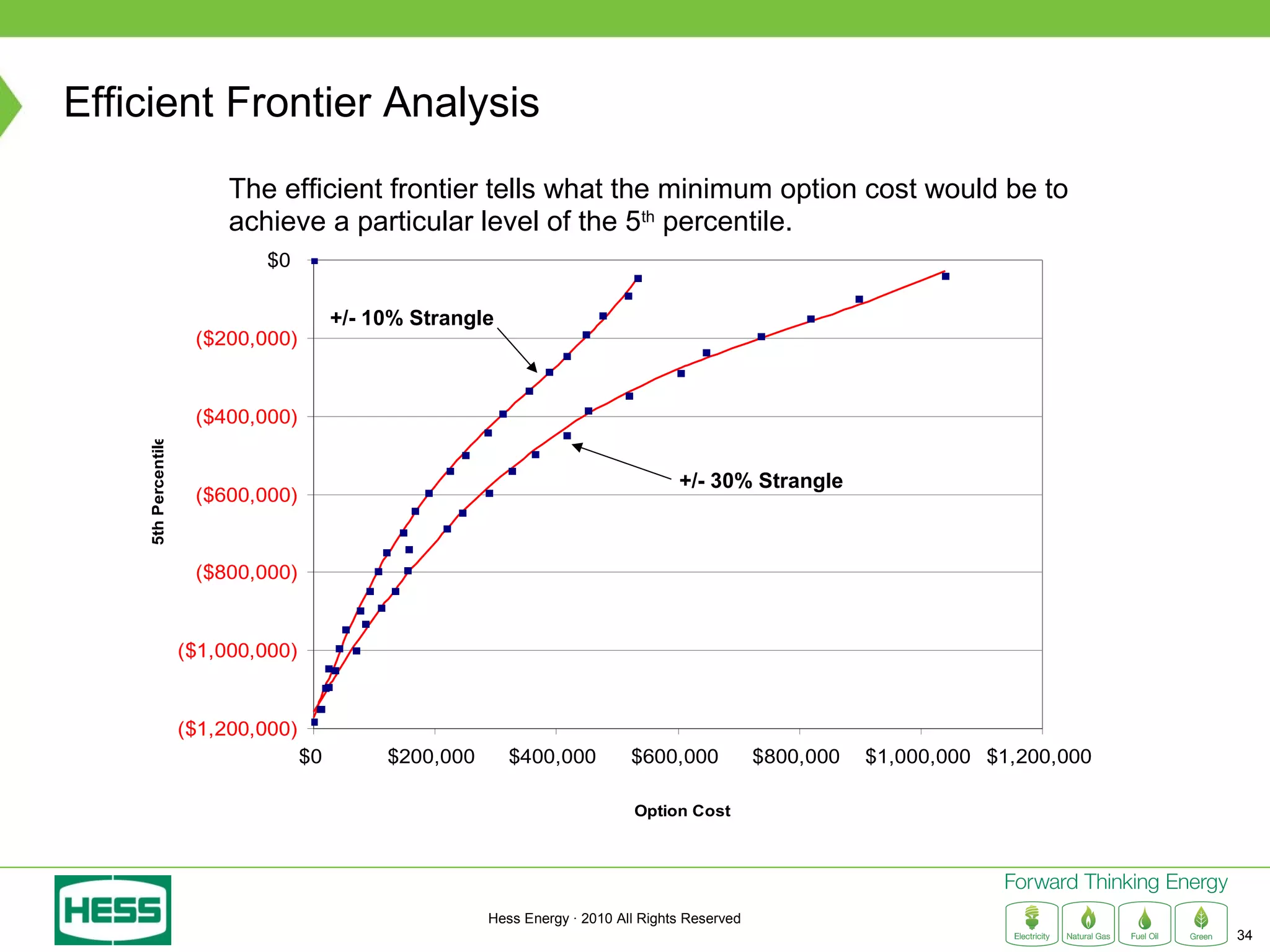


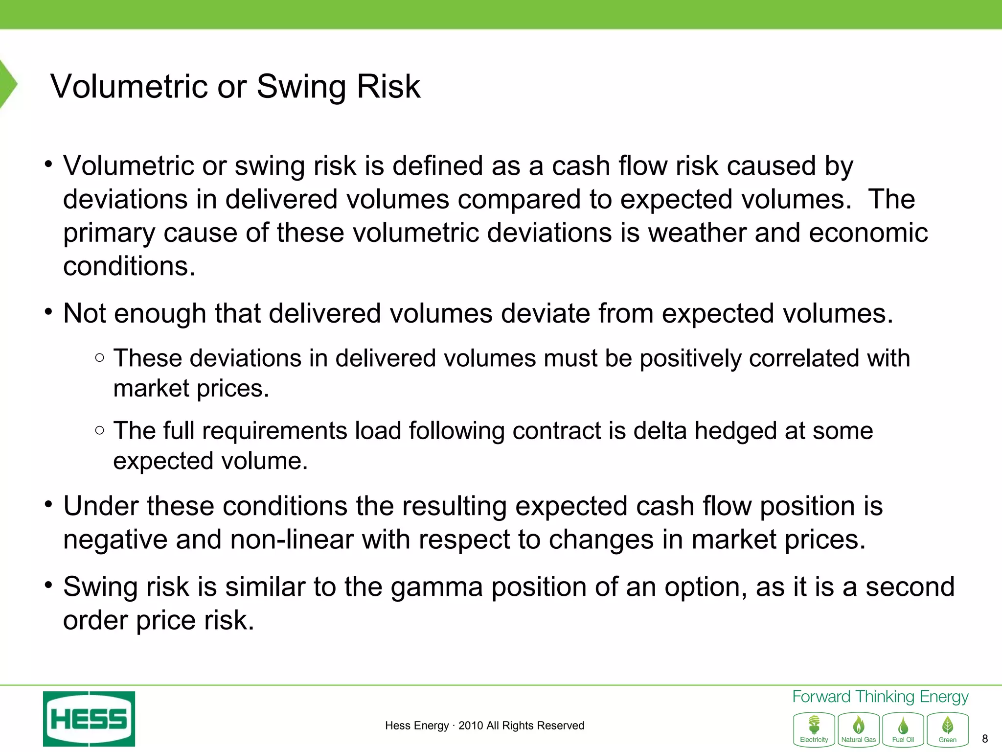
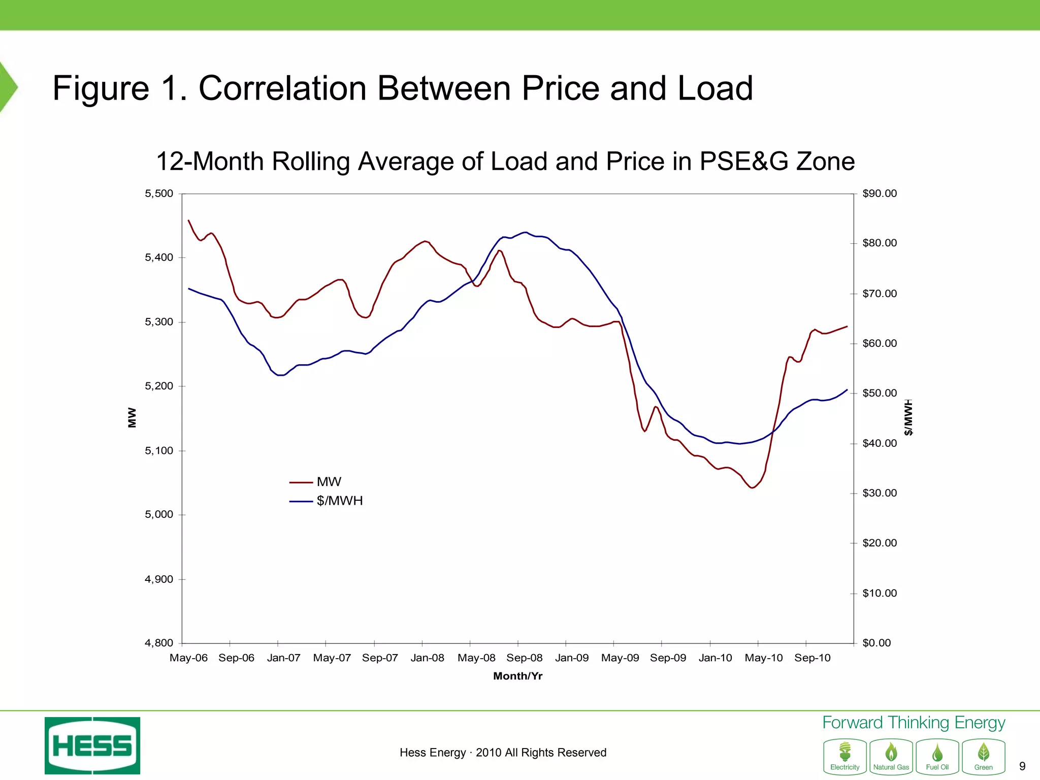
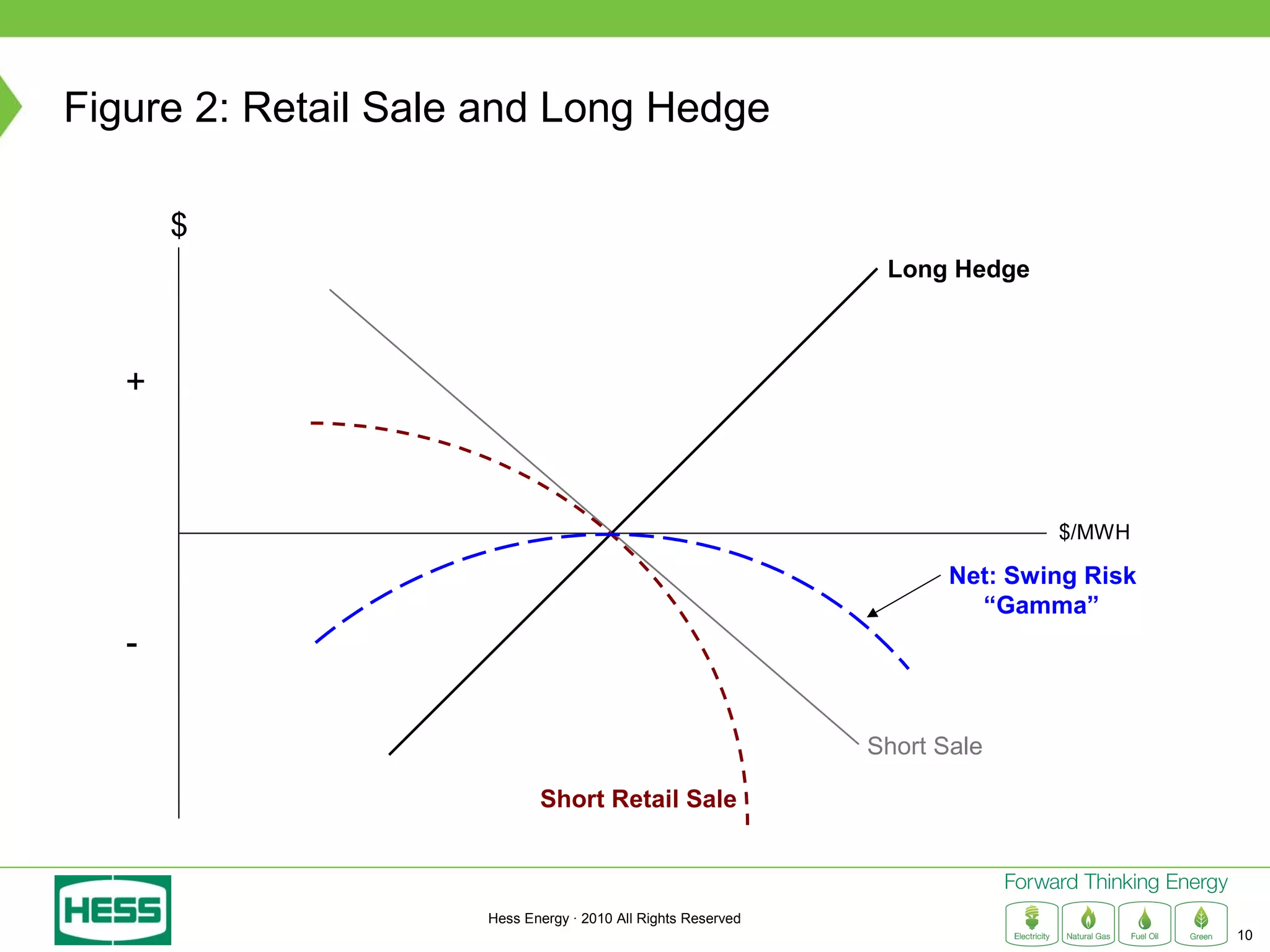
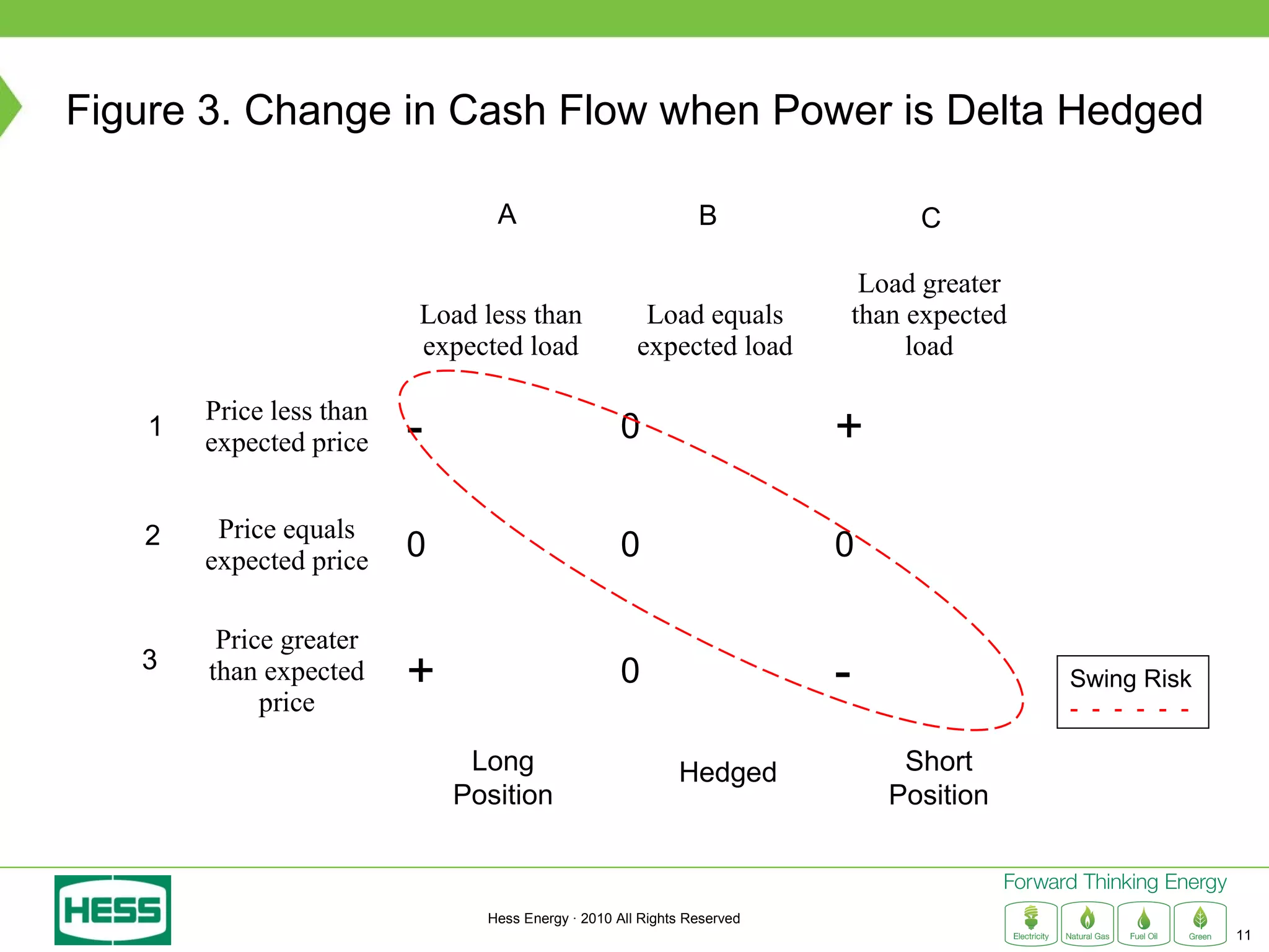
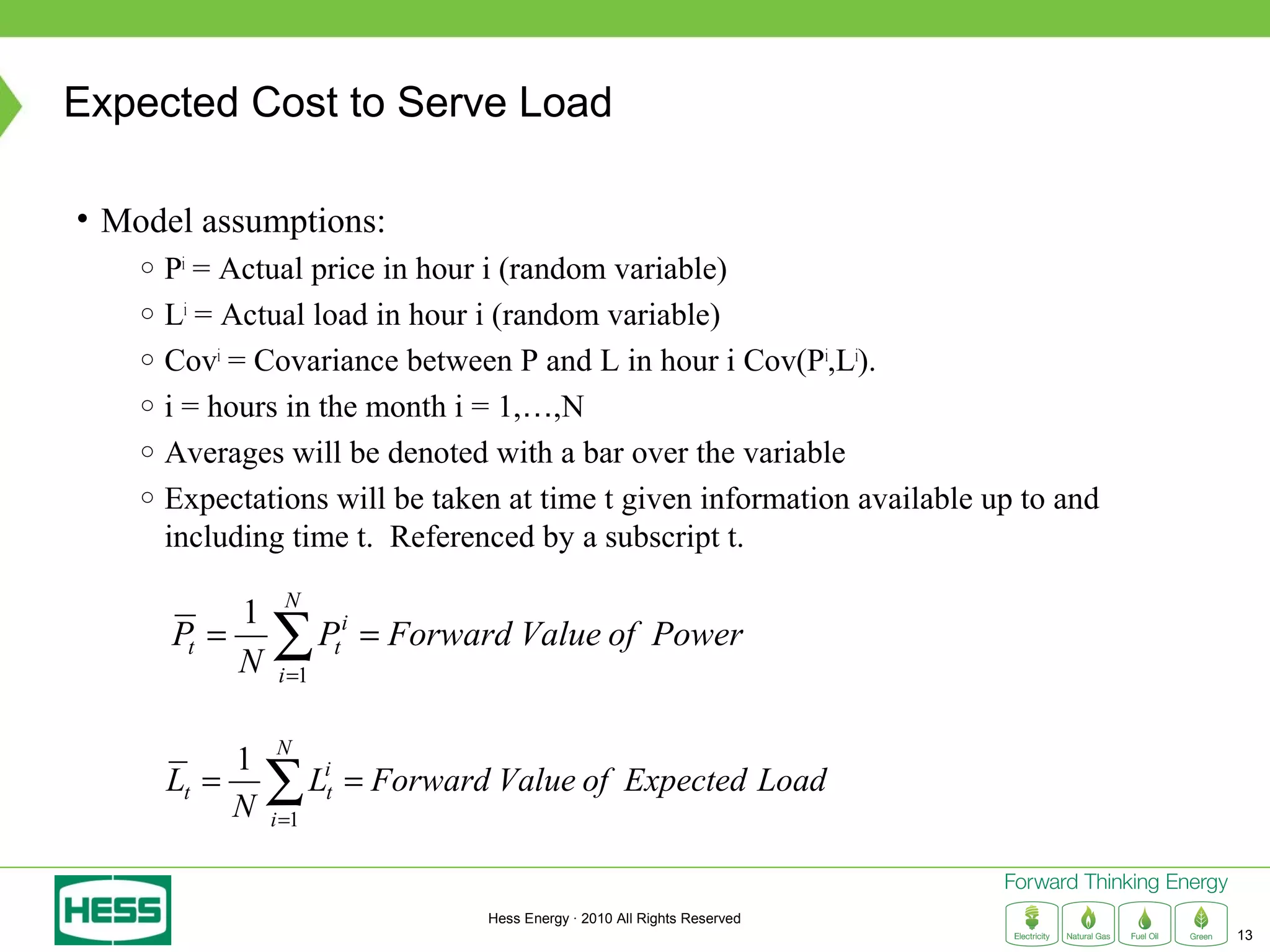
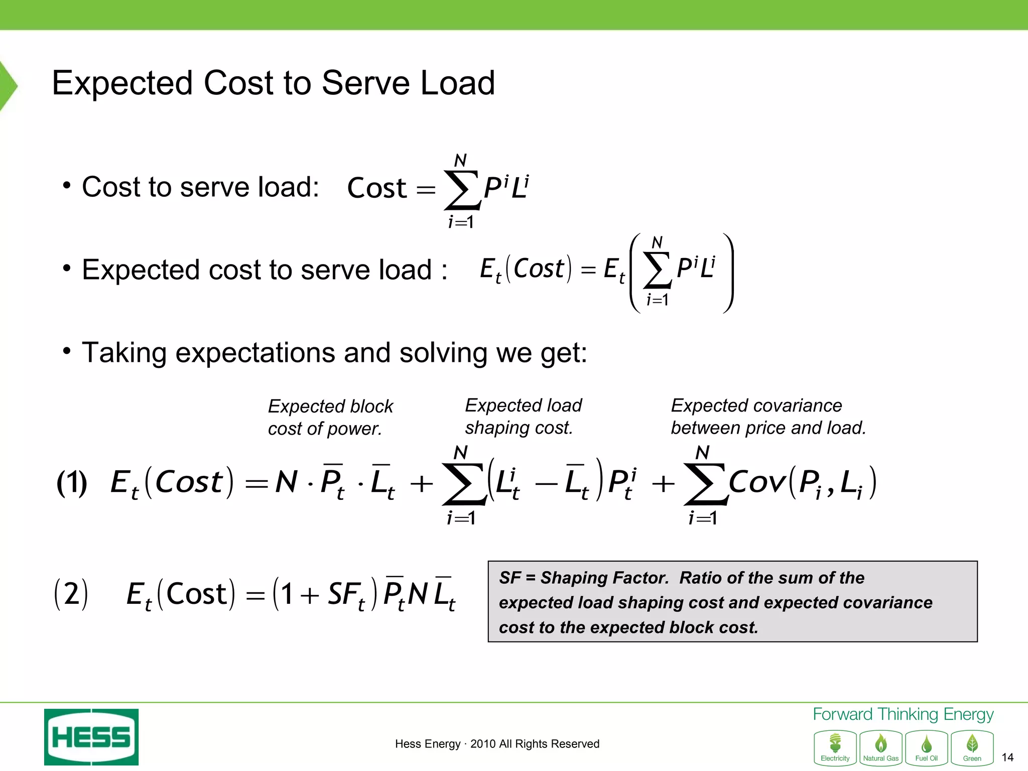
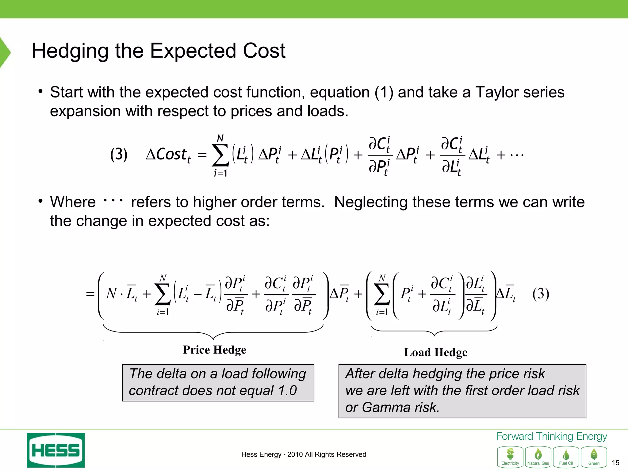
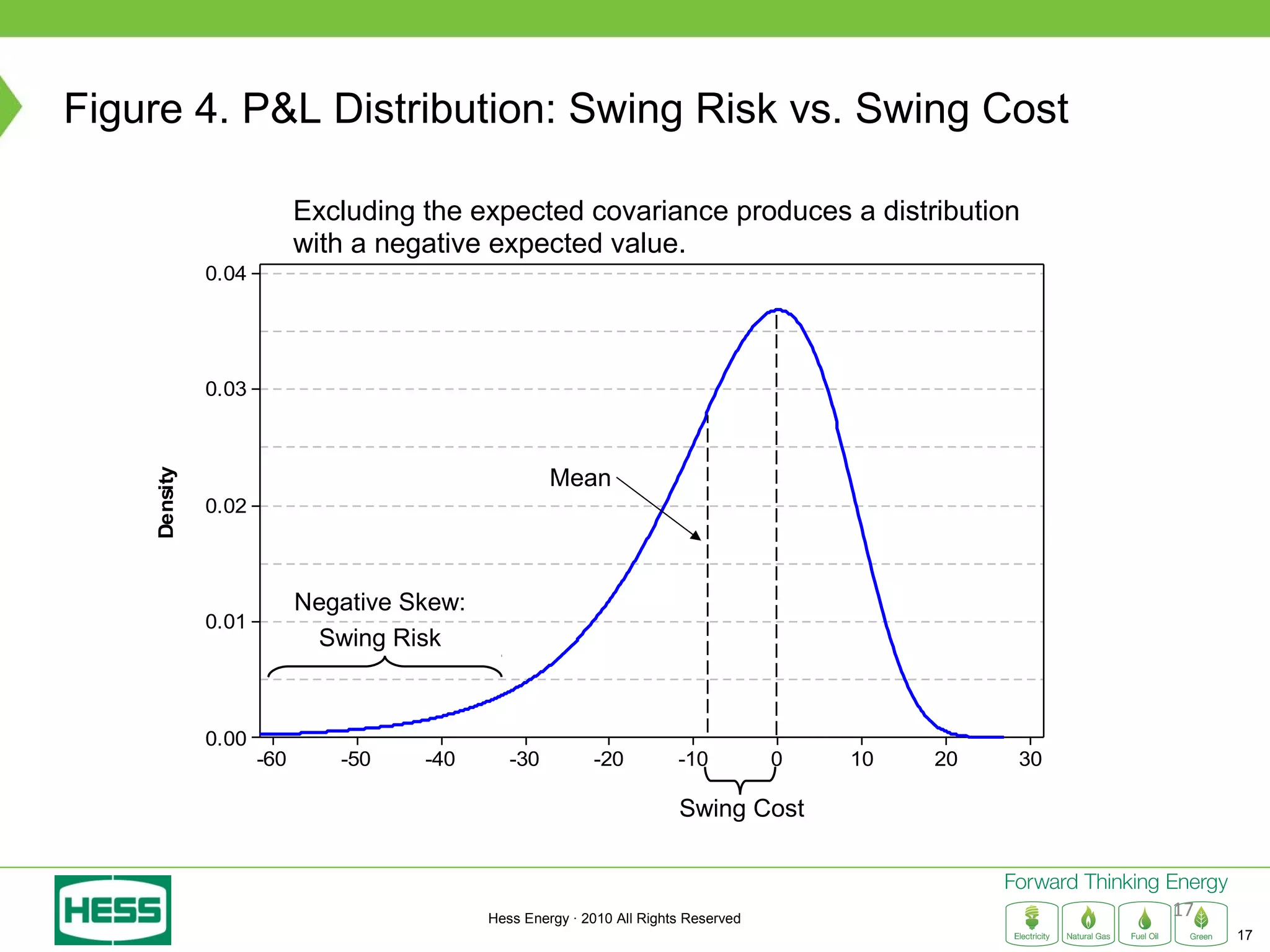
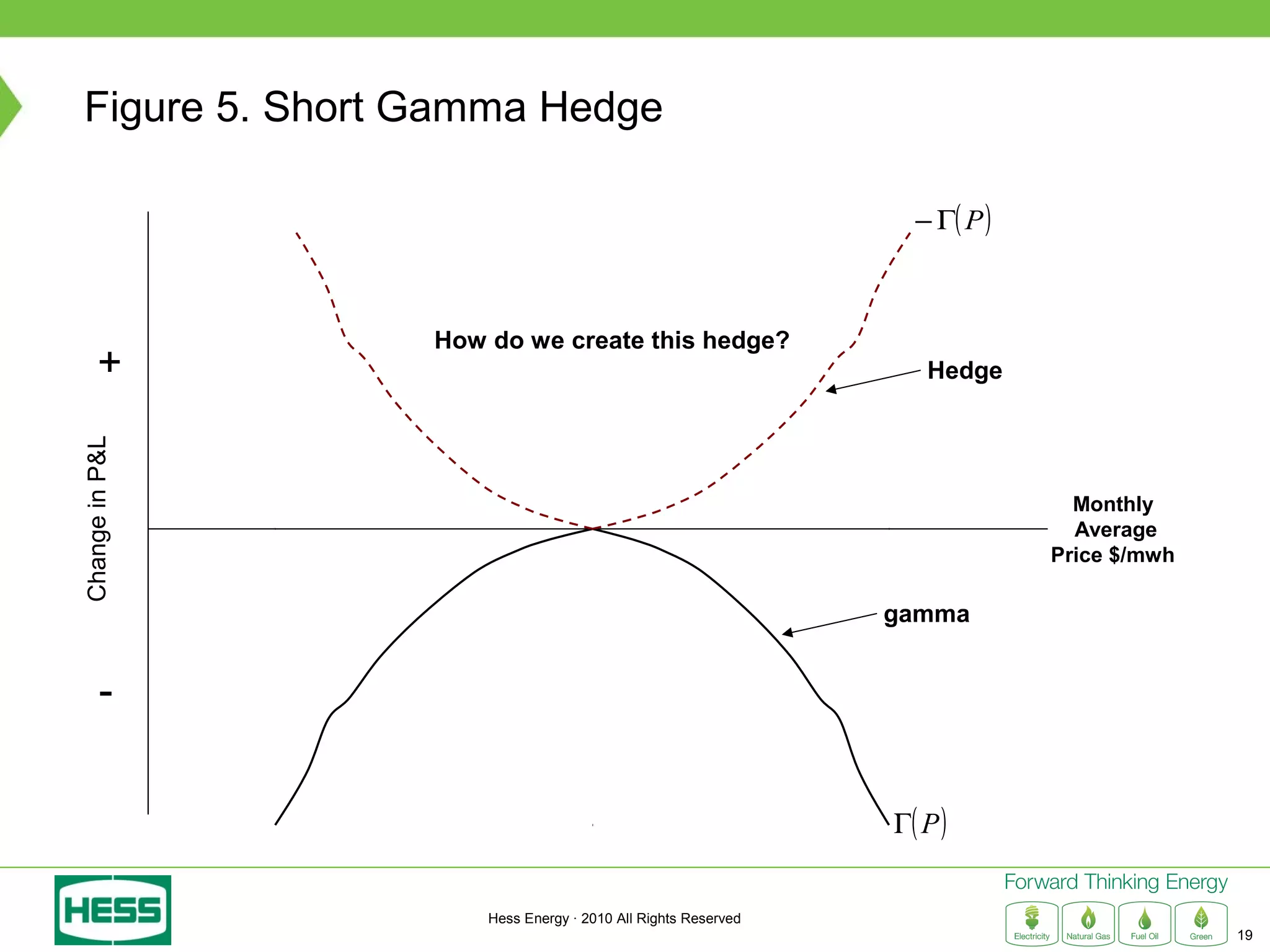
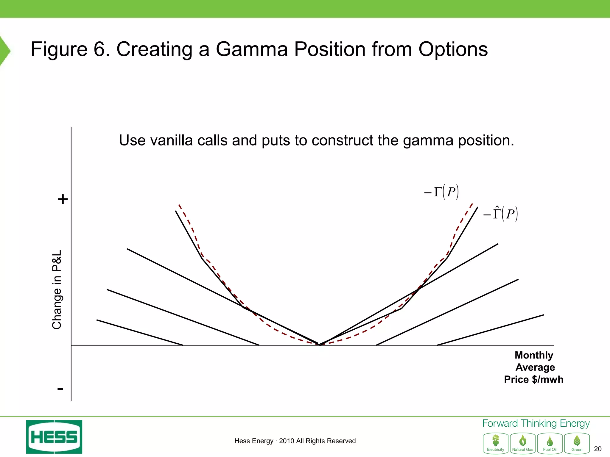
Modeling and Hedging the Risk in Retail Load Contracts discusses volumetric or "swing" risk in full requirements load following contracts for electricity. Swing risk is the cash flow risk from deviations in delivered load volumes from expected levels that are positively correlated with market prices. The document outlines how to estimate the expected cost of serving load including an expected "shaping factor" cost, describes delta hedging price risk but remaining exposed to swing risk, and proposes using options to construct a "gamma hedge" to manage swing risk. Regression analysis is used to estimate the relationship between historic load and price in order to model the gamma exposure and design an optimal options hedge.


