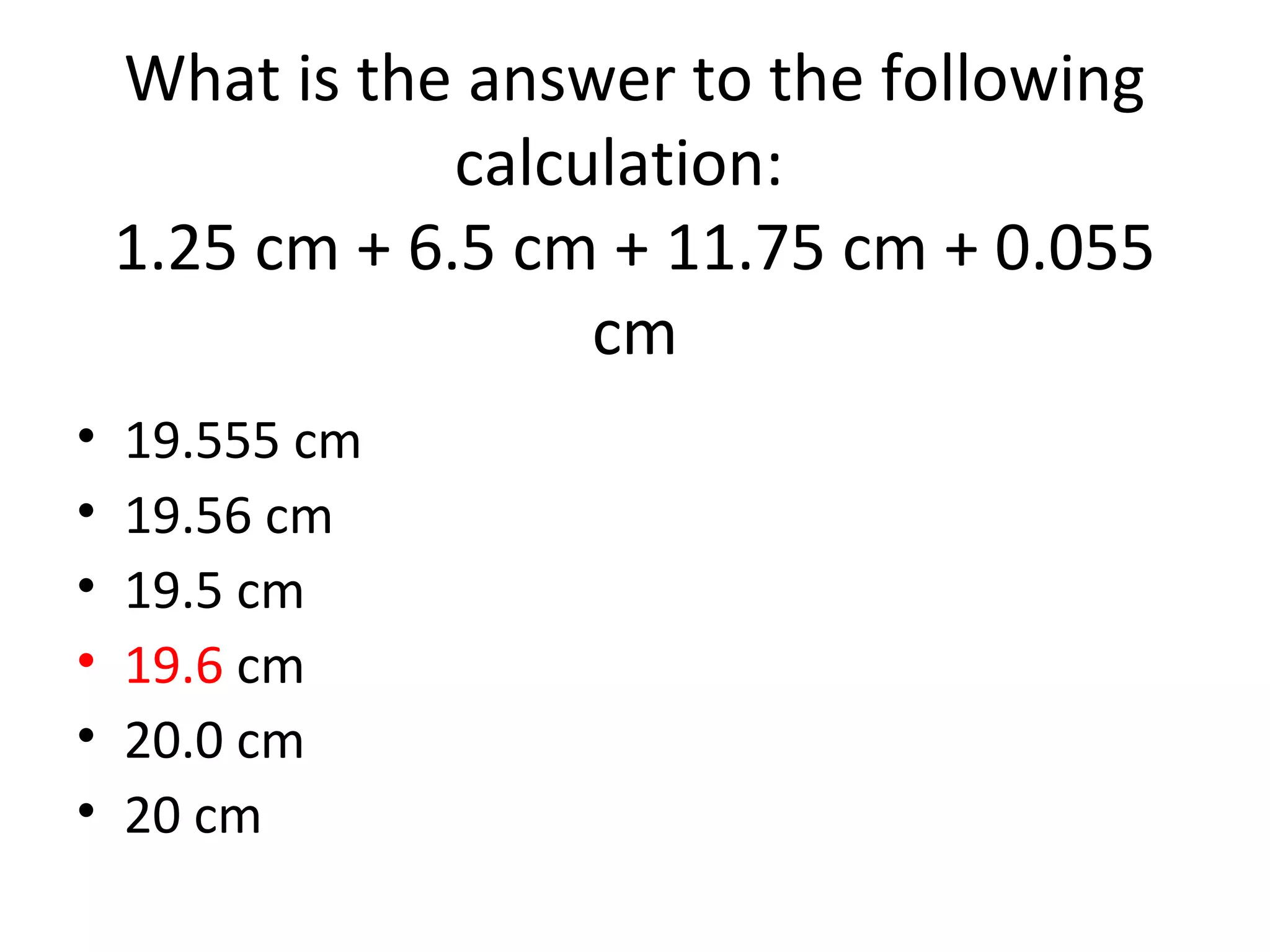
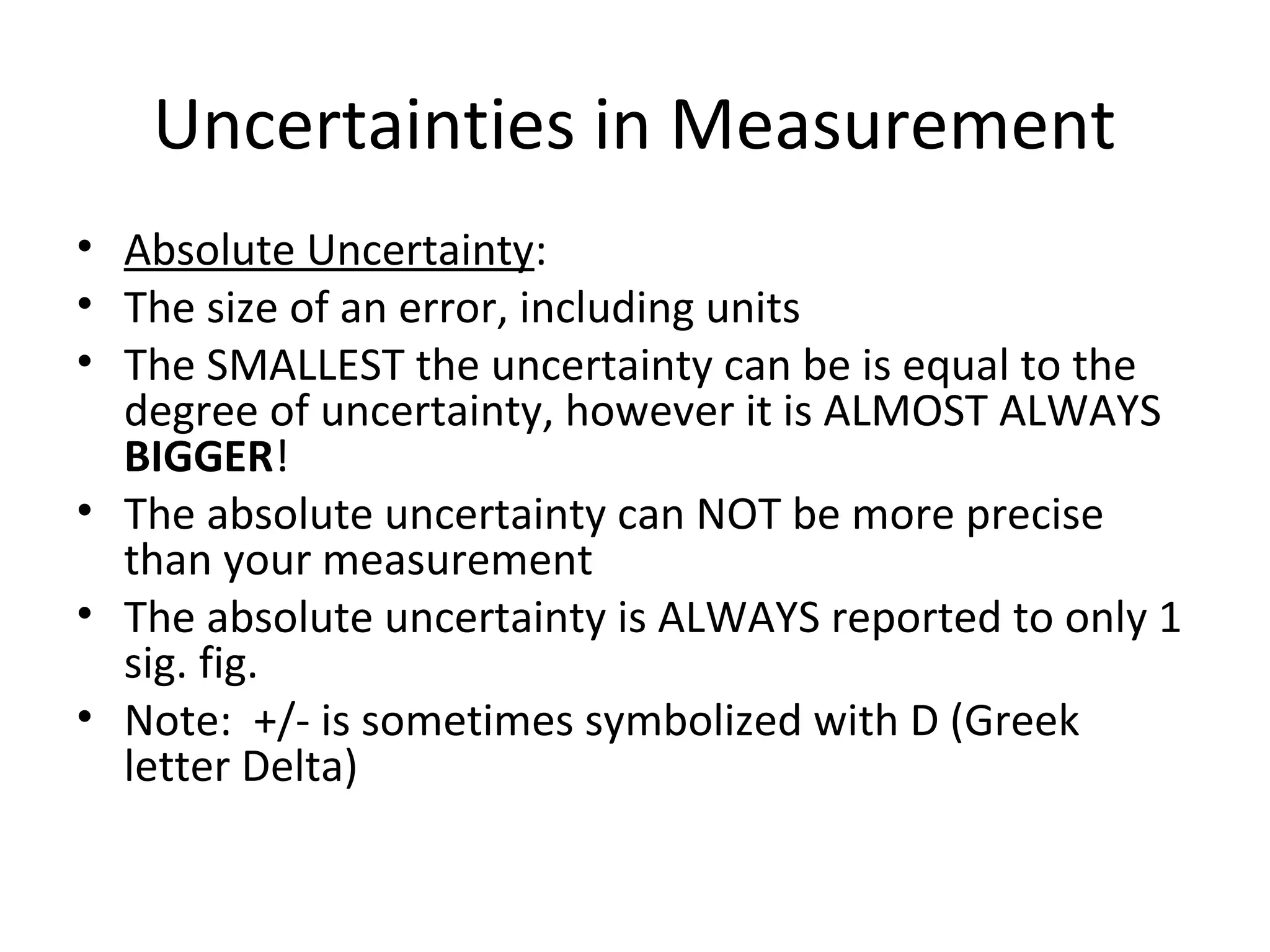
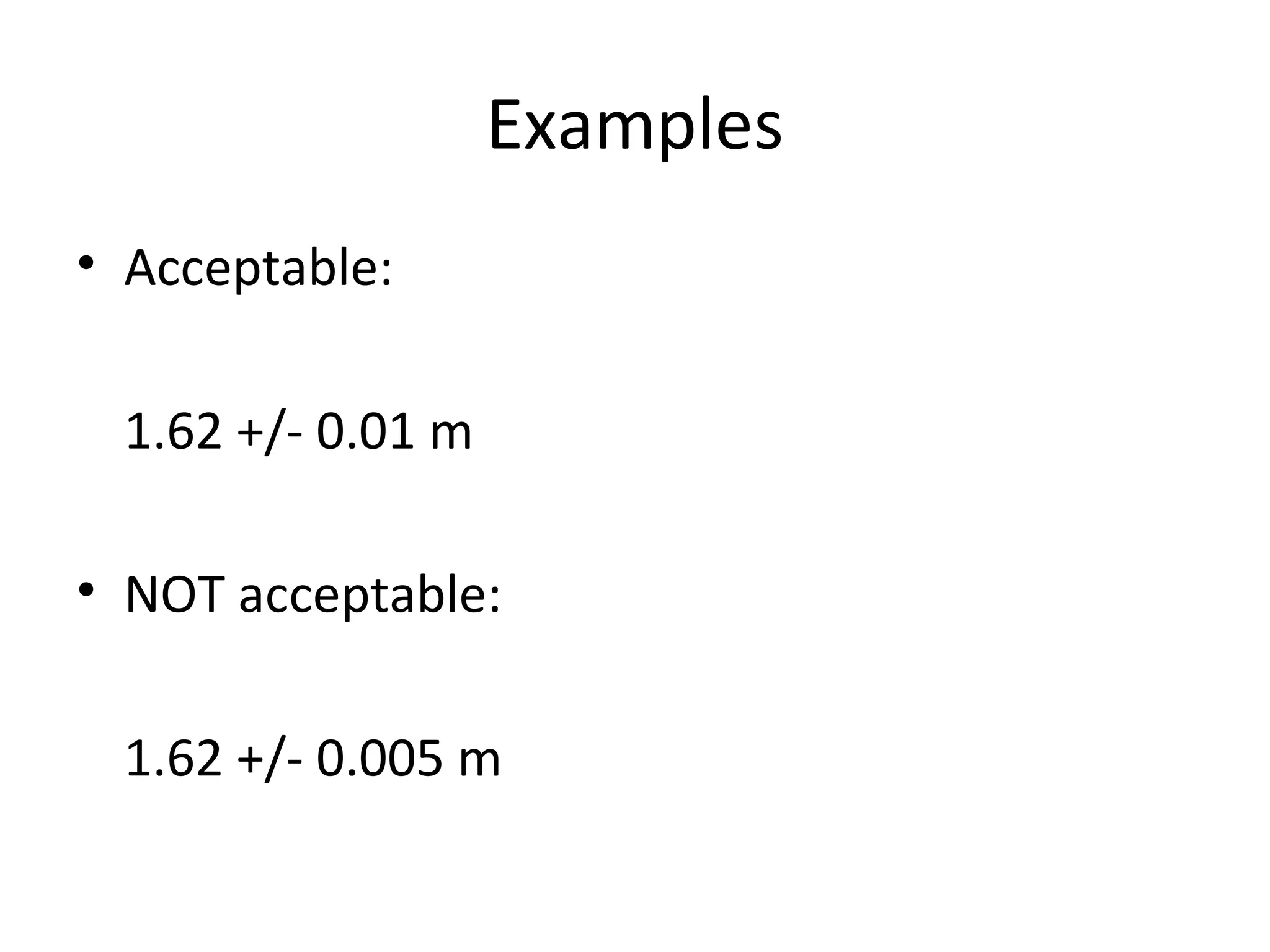
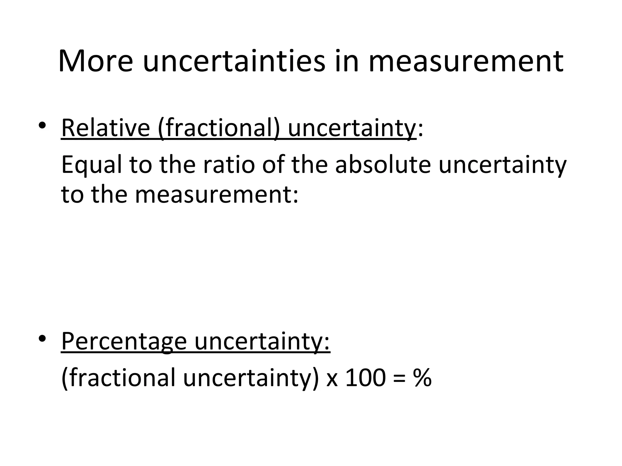
Errors and Uncertainties
in measurements and in calculations
Types of Experimental Errors
• Random Errors:
• A result of variations in the performance of the
instrument and/or the operator
• Do NOT consistently occur throughout a lab
• Some examples:
• Vibrations or air currents when measuring mass
• Inconsistent temperature (i.e. of the air) throughout a
lab
• Irregularities in object being measured (i.e. the wire is
not the same thickness at all points along its length)
• Human parallax error
Types of Experimental Errors
• So what can be done about random errors?
• Don’t rush through your measurements! Be
careful!
• Take as many trials as possible—the more
trials you do, the less likely one odd result will
impact your overall lab results
Types of Experimental Errors
• Systematic Errors:
• Errors that are inherent to the system or the
measuring instrument
• Results in a set of data to be centered around a value
that is different than the accepted value
• Some Examples:
• Non-calibrated (or poorly calibrated) measuring tools
• A “zero offset” on a measuring tool, requiring a “zero
correction”
• Instrument parallax error
Types of Experimental Errors
• What can be done to reduce these?
• Unfortunately, nothing…HOWEVER:
• We can account for the systematic errors
sometimes:
• i.e. if there’s a zero offset, make sure all your
data has been adjusted to account for that.
• Recognizing systematic errors will impact the
size of your absolute uncertainty (more
details soon )
Are these “errors”?
• Misreading the scale on a triple-beam balance
• Incorrectly transferring data from your rough
data table to the final, typed, version in your
report
• Miscalculating results because you did not
convert to the correct fundamental units
• Miscalculations because you use the wrong
equation
Are these “errors”?
• NONE of these are experimental errors
• They are MISTAKES
• What’s the difference?
• You need to check your work to make sure
these mistakes don’t occur…ask questions if
you need to (of your lab partner, me, etc.)
• Do NOT put mistakes in your error discussion
in the conclusion
How many significant figures are in the
following measurement:
415.2 cm
• 1
• 2
• 3
• 4
How many significant figures are in the
following measurement:
0.00065 s
• 2
• 3
• 4
• 5
How many significant figures are in the
following measurement:
1500 g
• 1
• 2
• 3
• 4
How many significant figures are in
the following measurement:
0.007250 W
• 7
• 5
• 4
• 3
How many significant figures are in the
following measurement:
105.00 cm
• 2
• 3
• 4
• 5
How many sig figs will be in the
answer to the following calculation:
1.25 cm + 6.5 cm + 11.75 cm + 0.055
cm
• 1
• 2
• 3
• 4
What is the answer to the following
calculation:
1.25 cm + 6.5 cm + 11.75 cm + 0.055
cm
• 19.555 cm
• 19.56 cm
• 19.5 cm
• 19.6 cm
• 20.0 cm
• 20 cm
What is the answer to the
following calculation:
25.50 m * 12.057 m * 0.095 m
• 29.2080825 m3
• 29.2081 m3
• 29.208 m3
• 29.21 m3
• 29.2 m3
• 29 m3
Significant Figures (sig. figs.)
• All digits in a measurement that are known for
certain, plus the first estimated (uncertain)
digit
• Sig figs give an indication of the degree of
precision for a measurement and/or a
calculation
• ONLY used when a number is (or is assumed
to be) a measurement
• EXACT quantities do not have “sig figs”
Sig Fig Rules—Know and USE these!!
• Rules for determining how many sig figs are in a
measurement:
• All non-zero values ARE significant
i.e. 54 mm has 2 s.f.; 5400 m has 2 s.f.
• All zeros between non-zero digits ARE significant
i.e. 504 N has 3 s.f.
• For numbers LESS THAN 1:
• Zeros directly after the decimal point are NOT
significant
i.e. 0.00565 J has 3 s.f.
Sig Fig Rules—Know and USE these!!
• A zero to the right of a decimal AND following a
non-zero digit IS significant
• 0.150 m has 3 s.f.; 15.0 kg has 3 s.f.;
• All other zeros are NOT significant
• Examples: How many sig figs in each of the
following?
• 15.035 cm
• 0.0560 s
• 35000 kg
Scientific notation and sig figs
• Use Scientific notation when you need to
specify how many zeros are significant
i.e. Write 1500 N with 3 s.f.
• The best way to do this is with scientific
notation: 1.50 x 10³
N
Write 10600 kg with 4 s.f.
Note on book problems
• Most of the problems in your book will have
values which look like they only have 1 s.f.
• Assume that all digits in book problems are
significant
i.e. if a problem says that an object has a mass
of 100 kg, please treat that as 3 s.f.
Sig. Figs in Calculations
• When adding or subtracting:
• Your answer must have the same degree of
precision as the least precise measurement
(that means…go to the fewest number of
decimal places)
i.e.:
24.2 g + 0.51 g + 7.134 g = 31.844 g  31.8 g
• When multiplying and dividing:
• The number of sig figs in the answer is equal
to the least number of sig figs in any of the
measurements used in the calculation
i.e. 3.22 cm * 12.34 cm * 1.8 cm = 71.52264
cm3
 72 cm3
Uncertainties in Measurement
• Limit of Reading:
• Equal to the smallest graduation of the scale
on an instrument
• Degree of Uncertainty:
• Equal to half the limit of reading
• Gives an indication of the precision of the
reading
Uncertainties in Measurement
• Absolute Uncertainty:
• The size of an error, including units
• The SMALLEST the uncertainty can be is equal to the
degree of uncertainty, however it is ALMOST ALWAYS
BIGGER!
• The absolute uncertainty can NOT be more precise
than your measurement
• The absolute uncertainty is ALWAYS reported to only 1
sig. fig.
• Note: +/- is sometimes symbolized with D (Greek
letter Delta)
Examples
• Acceptable:
1.62 +/- 0.01 m
• NOT acceptable:
1.62 +/- 0.005 m
More uncertainties in measurement
• Relative (fractional) uncertainty:
Equal to the ratio of the absolute uncertainty
to the measurement:
• Percentage uncertainty:
(fractional uncertainty) x 100 = %
Uncertainty Propagation
• When we perform calculations with
measurements that have uncertainties, there
is a certain amount of uncertainty in our
calculated answer as well.
• Carrying our errors through the calculations is
called “error propagation” or “uncertainty
propagation”
Rule 1: Addition/Subtraction
• When you are adding or subtracting values in
a calculation, the uncertainty in the calculated
answer is equal to the sum of the absolute
uncertainties for each measurement added: n
24.10 ± 0.05 g
+ 13.05 ± 0.02 g
= 37.15 ± 0.07 g
Rule #2: Multiplying/Dividing
• When multiplying or dividing, the uncertainty
in the calculated value is equal to the sum of
the percentage uncertainties for each of the
individual measurements:
• For example, let’s say we were to calculate
the volume from the following
measurements:
• (12.0 ± 0.2 cm)*(23.1 ± 0.2 cm)*(7.5 ± 0.1 cm)
• Step 1: determine the % uncertainty for each
measurement
• Step 2: Add all of the % uncertainties and
round to 1-2 sig figs (usually a whole number,
although if under 1 keep as a one s.f. decimal
percentage:
• Step 3: convert the percentage uncertainty in
your answer back to an absolute uncertainty:
(12.0 ± 0.2 cm)*(23.1 ± 0.2 cm)*(7.5 ± 0.1 cm)
= 2100 cm3
± 4%
0.04 x 2100 cm3
= 84 cm3
≈ 100cm3
• (note: since the precision of the measurement
and the uncertainty MUST BE THE SAME, always
go with the least precise of the two when
reporting your final answer.)
• V = 2100 ± 100 cm3

Errors and uncertainties

  • 1.
    Errors and Uncertainties inmeasurements and in calculations
  • 2.
    Types of ExperimentalErrors • Random Errors: • A result of variations in the performance of the instrument and/or the operator • Do NOT consistently occur throughout a lab • Some examples: • Vibrations or air currents when measuring mass • Inconsistent temperature (i.e. of the air) throughout a lab • Irregularities in object being measured (i.e. the wire is not the same thickness at all points along its length) • Human parallax error
  • 3.
    Types of ExperimentalErrors • So what can be done about random errors? • Don’t rush through your measurements! Be careful! • Take as many trials as possible—the more trials you do, the less likely one odd result will impact your overall lab results
  • 4.
    Types of ExperimentalErrors • Systematic Errors: • Errors that are inherent to the system or the measuring instrument • Results in a set of data to be centered around a value that is different than the accepted value • Some Examples: • Non-calibrated (or poorly calibrated) measuring tools • A “zero offset” on a measuring tool, requiring a “zero correction” • Instrument parallax error
  • 5.
    Types of ExperimentalErrors • What can be done to reduce these? • Unfortunately, nothing…HOWEVER: • We can account for the systematic errors sometimes: • i.e. if there’s a zero offset, make sure all your data has been adjusted to account for that. • Recognizing systematic errors will impact the size of your absolute uncertainty (more details soon )
  • 6.
    Are these “errors”? •Misreading the scale on a triple-beam balance • Incorrectly transferring data from your rough data table to the final, typed, version in your report • Miscalculating results because you did not convert to the correct fundamental units • Miscalculations because you use the wrong equation
  • 7.
    Are these “errors”? •NONE of these are experimental errors • They are MISTAKES • What’s the difference? • You need to check your work to make sure these mistakes don’t occur…ask questions if you need to (of your lab partner, me, etc.) • Do NOT put mistakes in your error discussion in the conclusion
  • 8.
    How many significantfigures are in the following measurement: 415.2 cm • 1 • 2 • 3 • 4
  • 9.
    How many significantfigures are in the following measurement: 0.00065 s • 2 • 3 • 4 • 5
  • 10.
    How many significantfigures are in the following measurement: 1500 g • 1 • 2 • 3 • 4
  • 11.
    How many significantfigures are in the following measurement: 0.007250 W • 7 • 5 • 4 • 3
  • 12.
    How many significantfigures are in the following measurement: 105.00 cm • 2 • 3 • 4 • 5
  • 13.
    How many sigfigs will be in the answer to the following calculation: 1.25 cm + 6.5 cm + 11.75 cm + 0.055 cm • 1 • 2 • 3 • 4
  • 14.
    What is theanswer to the following calculation: 1.25 cm + 6.5 cm + 11.75 cm + 0.055 cm • 19.555 cm • 19.56 cm • 19.5 cm • 19.6 cm • 20.0 cm • 20 cm
  • 15.
    What is theanswer to the following calculation: 25.50 m * 12.057 m * 0.095 m • 29.2080825 m3 • 29.2081 m3 • 29.208 m3 • 29.21 m3 • 29.2 m3 • 29 m3
  • 16.
    Significant Figures (sig.figs.) • All digits in a measurement that are known for certain, plus the first estimated (uncertain) digit • Sig figs give an indication of the degree of precision for a measurement and/or a calculation • ONLY used when a number is (or is assumed to be) a measurement • EXACT quantities do not have “sig figs”
  • 17.
    Sig Fig Rules—Knowand USE these!! • Rules for determining how many sig figs are in a measurement: • All non-zero values ARE significant i.e. 54 mm has 2 s.f.; 5400 m has 2 s.f. • All zeros between non-zero digits ARE significant i.e. 504 N has 3 s.f. • For numbers LESS THAN 1: • Zeros directly after the decimal point are NOT significant i.e. 0.00565 J has 3 s.f.
  • 18.
    Sig Fig Rules—Knowand USE these!! • A zero to the right of a decimal AND following a non-zero digit IS significant • 0.150 m has 3 s.f.; 15.0 kg has 3 s.f.; • All other zeros are NOT significant • Examples: How many sig figs in each of the following? • 15.035 cm • 0.0560 s • 35000 kg
  • 19.
    Scientific notation andsig figs • Use Scientific notation when you need to specify how many zeros are significant i.e. Write 1500 N with 3 s.f. • The best way to do this is with scientific notation: 1.50 x 10³ N Write 10600 kg with 4 s.f.
  • 20.
    Note on bookproblems • Most of the problems in your book will have values which look like they only have 1 s.f. • Assume that all digits in book problems are significant i.e. if a problem says that an object has a mass of 100 kg, please treat that as 3 s.f.
  • 21.
    Sig. Figs inCalculations • When adding or subtracting: • Your answer must have the same degree of precision as the least precise measurement (that means…go to the fewest number of decimal places) i.e.: 24.2 g + 0.51 g + 7.134 g = 31.844 g  31.8 g
  • 22.
    • When multiplyingand dividing: • The number of sig figs in the answer is equal to the least number of sig figs in any of the measurements used in the calculation i.e. 3.22 cm * 12.34 cm * 1.8 cm = 71.52264 cm3  72 cm3
  • 23.
    Uncertainties in Measurement •Limit of Reading: • Equal to the smallest graduation of the scale on an instrument • Degree of Uncertainty: • Equal to half the limit of reading • Gives an indication of the precision of the reading
  • 24.
    Uncertainties in Measurement •Absolute Uncertainty: • The size of an error, including units • The SMALLEST the uncertainty can be is equal to the degree of uncertainty, however it is ALMOST ALWAYS BIGGER! • The absolute uncertainty can NOT be more precise than your measurement • The absolute uncertainty is ALWAYS reported to only 1 sig. fig. • Note: +/- is sometimes symbolized with D (Greek letter Delta)
  • 25.
    Examples • Acceptable: 1.62 +/-0.01 m • NOT acceptable: 1.62 +/- 0.005 m
  • 26.
    More uncertainties inmeasurement • Relative (fractional) uncertainty: Equal to the ratio of the absolute uncertainty to the measurement: • Percentage uncertainty: (fractional uncertainty) x 100 = %
  • 27.
    Uncertainty Propagation • Whenwe perform calculations with measurements that have uncertainties, there is a certain amount of uncertainty in our calculated answer as well. • Carrying our errors through the calculations is called “error propagation” or “uncertainty propagation”
  • 28.
    Rule 1: Addition/Subtraction •When you are adding or subtracting values in a calculation, the uncertainty in the calculated answer is equal to the sum of the absolute uncertainties for each measurement added: n 24.10 ± 0.05 g + 13.05 ± 0.02 g = 37.15 ± 0.07 g
  • 29.
    Rule #2: Multiplying/Dividing •When multiplying or dividing, the uncertainty in the calculated value is equal to the sum of the percentage uncertainties for each of the individual measurements: • For example, let’s say we were to calculate the volume from the following measurements: • (12.0 ± 0.2 cm)*(23.1 ± 0.2 cm)*(7.5 ± 0.1 cm)
  • 30.
    • Step 1:determine the % uncertainty for each measurement • Step 2: Add all of the % uncertainties and round to 1-2 sig figs (usually a whole number, although if under 1 keep as a one s.f. decimal percentage:
  • 31.
    • Step 3:convert the percentage uncertainty in your answer back to an absolute uncertainty: (12.0 ± 0.2 cm)*(23.1 ± 0.2 cm)*(7.5 ± 0.1 cm) = 2100 cm3 ± 4% 0.04 x 2100 cm3 = 84 cm3 ≈ 100cm3 • (note: since the precision of the measurement and the uncertainty MUST BE THE SAME, always go with the least precise of the two when reporting your final answer.) • V = 2100 ± 100 cm3