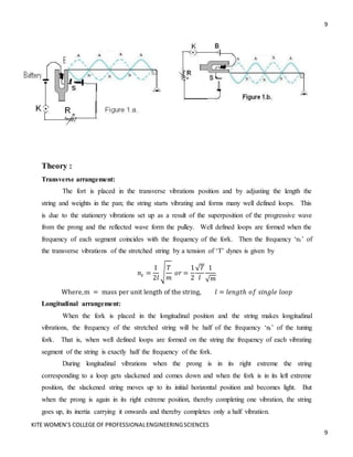
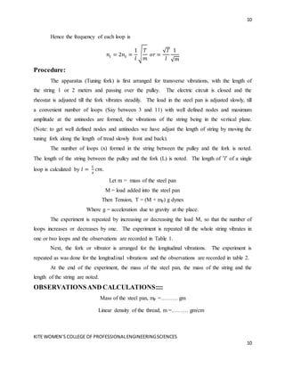
This document contains instructions and procedures for Experiment 2 which involves studying normal modes in a string using forced vibrations in rods (Melde's experiment). The aim is to determine the frequency of a vibrating bar or electrically maintained tuning fork. It describes the apparatus, which includes a tuning fork, stand, pan, weights, and connecting wires. It provides the theory behind determining the transverse and longitudinal frequencies of a stretched string attached to a vibrating tuning fork. The procedure involves arranging the tuning fork for transverse and longitudinal vibrations and adjusting the string and weights to form distinct loops. Key measurements taken include the number of loops formed and the total string length to calculate the length of a single loop.
1. 1
KITE WOMEN’S COLLEGE OF PROFESSIONALENGINEERINGSCIENCES
1
Engineering Physics
Laboratory Manual
CONTENTS
Instructions for Laboratory ……….2
Bibliography ……….3
Experiment 1: Determination of Rigidity modulus of a material – Torsional pendulum ……..4
Experiment 2: Melde’s Experiment – Transverse and Longitudinal Modes ……..8
Experiment 3: Time Constant of RC Circuit ……….12
Experiment 4: Resonance in LCR circuit ……….15
Experiment 5: Evaluation of Numerical Aperture of a given fiber ……….20
Experiment 6: Losses in Optical fiber ………22
Experiment 7: Characteristics of LED source ………25
Experiment 8: Diffraction at a Single slit (Laser) ………28
Experiment 9: Magnetic field along the axis of a current carrying coil. ………31
Experiment 10: Determination of Energy Gap of Semiconductor. ………35
Experiment 11: Characteristics of LASER source ………38
2. 2
KITE WOMEN’S COLLEGE OF PROFESSIONALENGINEERINGSCIENCES
2
Instructions for Laboratory
The objective of the laboratory is learning. The experiments are designed to illustrate phenomena
in different areas of Physics and to expose you to measuring instruments. Conduct the experiments
with interest and an attitude of learning.
You need to come well prepared for the experiment
Work quietly and carefully (the whole purpose of experimentation is to make reliable
measurements!) and equally share the work with your partners.
Be honest in recording and representing your data. Never make up readings or doctor them to get a
better fit for a graph. If a particular reading appears wrong repeat the measurement carefully. In
any event all the data recorded in the tables have to be faithfully displayed on the graph.
All presentations of data, tables and graphs calculations should be neatly and carefully done.
Bring necessary graph papers for each of experiment. Learn to optimize on usage of graph papers.
Graphs should be neatly drawn with pencil. Always label graphs and the axes and display units.
If you finish early, spend the remaining time to complete the calculations and drawing graphs.
Come equipped with calculator, scales, pencils etc.
Do not fiddle idly with apparatus. Handle instruments with care. Report any breakage to the
Instructor. Return all the equipment you have signed out for the purpose of your experiment.
3. 3
KITE WOMEN’S COLLEGE OF PROFESSIONALENGINEERINGSCIENCES
3
Bibliography
Here is a short list of references to books which may be useful for further reading in Physics or
instrumentation relevant to the experiments. Also included are some references to books of general
interest with regard to science and experimentation.
1. "Fundamentals of Physics", 6th Ed., D. Halliday, R. Resnick and J. Walker, John Wiley and Sons, Inc.,
New York, 2001.
2. "Engineering Physics” Basic Edition of S.L.Gaur and Gupta Text Book.
3. Engineering Physics Lab manual from Gurunanak Engineering College, Ibrahimpatnam.
4. Engineering physics Lab manual from Vivekananda Group of Institutions, Batasingaram.
5. Engineering Physics Lab manual from Spoorthy Engineering College, Gurramguda.
4. 4
KITE WOMEN’S COLLEGE OF PROFESSIONALENGINEERINGSCIENCES
4
EXPERIMENT 1
DETERMINATION OF RIGIDITY MODULUS OF THE MATERIAL
OF A WIRE
(Torsional pendulum)
Aim: To determine the Modulus of rigidity of the material of the given wire using a torsional pendulum.
Apparatus: Torsional pendulum (A Circular brass disc provided with a chuck and nut at its centre, steel
wire or brass wire or copper wire any one, another chuck and nut fixed to a wall bracket), Stop watch,
Screw gauge, Vernier Calipers, Meter scale.
Description: The torsional pendulum consists of uniform circular metal disc of about 8 to 10cm diameter
with 1 or 2 cm thickness, suspended by a wire at the centre of the chuck at the centre of the disc and upper
end is gripped into another chuck which is fixed to a wall bracket.
Theory: When the disc is rotated in a horizontal plane to the radial position then the wire gets twisted.
Wire will exert a torque on the disc tending to returns it to the first position. This is the restoring torque.
For small twists, the restoring torque is proportional to the amount of twist or the angular displacement
(From hook’s law) so that
Let be the angle through which the wire is twisted. “a” is the radius of the
Wire, ‘l’ is the length of the wire between chuck and ‘η’ is the rigidity of
Modulus of the material of the wire, Then the restoring couple set up in it is equal to
4
. . .
2
n a
c
l
4
( . . )
2
a n
c
l
-------- Where ‘c’ is the Torsional Constant
(Twisting couple per unit (radian) twist of the wire).
This produces an angular acceleration (dw/dt) in the disc
Therefore if “I” is the moment of inertia of the disc about the wire we have
I. .
dw
c
dt
dw c
dt I
1
1
5. 5
KITE WOMEN’S COLLEGE OF PROFESSIONALENGINEERINGSCIENCES
5
i.e Negative sign shows that torque is directed opposite to the angular displacement’’, the angular
acceleration (
dw
dt
) of the angular displacement() and therefore its motion is simple harmonic hence time
period is given by
T= 2π
I
c
-----------------------
From & 4 2
8 I l
n
a T
In case of a circular disc whose geometric axes coincide with the axis of rotation. The moment of inertia
“I” is given by I=
2
2
MR
where M is the mass of disc and “R” is the radius of the disc.
Procedure:
The circular metal disc is suspended. The length of the wire between the chucks is adjusted to
90cm. When the disc is in equilibrium position, a small mark is made on the curved edge of the disc. This
marking will help to note the number of oscillations made by the disc when the disc oscillates. The disc is
set to oscillate by slowly turning the disc through a small angle.
When the disc is oscillating the time taken for 10 oscillations is noted with the help of a stopwatch
and recorded in the observations table in trail 1. The procedure is repeated for the same length of the wire
and again the time taken for 10 oscillations is noted and recorded in the observations table in trail 2. From
trail 1 and 2 the mean time for 10 oscillations is obtained. The time period (T) i.e. the time taken for one
oscillation is calculated.
The experiment is repeated, by decreasing the length of the wire in steps of 10 cm and the results
are tabulated in table.
The radius of the wire ‘a’ is to be found accurately with the help of a screw gauge since it occurs
as the fourth power in final equation. The radius and the mass of the disc are found with a vernier calipers
and a rough balance respectively.
The mean value of (l/T2) is substituted in final equation and η is calculated.
2
1
2
2
2
6. 6
KITE WOMEN’S COLLEGE OF PROFESSIONALENGINEERINGSCIENCES
6
A graph is also drawn with ‘l’ on the x - axis and T2 on the y – axis. It will linear as shown in the
figure. From the graph, the value of T2 for as large as a value of ‘l’ is noted and this value of (l/T2) is
substituted in final equation and the rigidity of the modulus of material of the material of the wire η is
calculated.
Model Graph:
Observations:
Mass of the disc : M = _______________gm
Radius of the disc : R = ______________cm
Average radius of the wire : a = ___________cm.
Table – 1: Determination of 2
l
T
Sl.No
Length of Wire
l ( cm)
Time for 20 oscillation Time Per one
oscillation
T= (t/20)
2
l
T
Trial1 Trail2 Mean (t) T T2
1 90
2 80
3 70
4 60
5 50
6 40
Y
X
l
T2
7. 7
KITE WOMEN’S COLLEGE OF PROFESSIONALENGINEERINGSCIENCES
7
Table – 2: To measure the radius of the disc with Vernier calipers.
L.C. of Vernier Calipers = 1 M.S.D / Total V.S.D. =1/10 = 0.1mm = 0.01cm
S.No.
Main Scale reading
(MSR)(cm)
A
Vernier
coincidence
(V.C)
V.C. x L.C. = B
(cm)
Diameter
A + B (cm)
Table – 3: To measure the radius of the wire with screw gauge.
Pitch of the screw = Distance travelled by the screw / Number of rotations
L.C. of Screw Gauge =
𝑷𝒊𝒕𝒄𝒉 𝒐𝒇 𝒕𝒉𝒆 𝒔𝒄𝒓𝒆𝒘
𝑻𝒐𝒕𝒂𝒍 𝒏𝒖𝒎𝒃𝒆𝒓 𝒐𝒇 𝑯𝒆𝒂𝒅 𝒔𝒄𝒂𝒍𝒆 𝒅𝒊𝒗𝒊𝒔𝒊𝒐𝒏𝒔
=
𝟏
𝟏𝟎𝟎
= 0.01mm = 0.001cm
Zero Error = Correction =
S.No.
Reading on the
pitch Scale
A(mm)
Head scale
Reading
(H.S.R)
Corrected Head
Scale Reading
(C.H.S.R)
C.H.S.R x L.C.
B(mm)
Diameter of the
wire
A + B (mm)
Calculations:
Formulae: Rigidity Modulus of wire η =
4𝜋
𝑎4
𝑀𝑟2 𝑙
𝑇2
Precautions: 1.The length between the chucks should be measured carefully.
2. Screw gauge and Vernier Calipers readings have to be noted with accuracy.
Result: The rigidity modulus of the material of given wire is determined using Torsional pendulum.
Rigidity modulus of the given wire is
1. From table η =
2. From graph η =
8. 8
KITE WOMEN’S COLLEGE OF PROFESSIONALENGINEERINGSCIENCES
8
EXPERIMENT 2
STUDY OF NORMAL MODES IN A STRING USING FORCED VIBRATIONS IN RODS
(MELDE’S EXPERIMENT)
Aim: To determine the frequency of vibrating bar or electrically maintained Tuning fork.
Apparatus:• Electrically maintained tuning fork, A stand with clamp and pulley, A steel pan, A weight
box, Analytical Balance, A battery with eliminator, connecting wires, meter scale and thread.
Description:
An electrically maintained tuning fork consists of an electro – magnet between the two prongs of a
tuning fork without touching either of prongs, as shown in figure 1. To one of the prongs a thin brass plate
with an adjustable screw is riveted on it. By adjusting screw, contact is established with the thin brass
plate.
Electrical connections are made as shown in figure 1. When plug is inserted in the key, the circuit
is completed and the electrical current flows through the circuit energizing the electromagnet there by
pulling both the prongs inwards. The circuit is broken immediately at the point S, the electro – magnet
loses its magnetism and the prongs fly back to its original position. Consequently contact is once again
established at S, the circuit is closed and the process repeats automatically as before. This causes the
prongs of the tuning fork to vibrate.
One end of a thin thread is connected to a small screw provided on one of the prongs of the tuning
fork. The other end of the tread is connected to a steel pan and the thread is passed over a small friction
free pulley fixed on to a stand kept at a distance of 1 to 2 meters from the fork. Small weights are placed
in the steel pan so that sufficient tension is created to the string. The tension in the string can be altered by
changing the weights in the steel pan.
The tuning fork is arranged as shown in figure 1.a. for longitudinal vibrations, i.e. the vibrations of
the prong are parallel to the length of the string. After noting the observations in the position, the tuning
fork is arranged as shown in figure 1.b. for transverse vibrations, i.e. the vibrations of the prong are
perpendicular to the length of the string.
It is to be noted that in both the cases, the stretched string should at right angles to its length (In the
both cases) in case the stretched string after forming loops rotates, then small weights are either to be
added into the pan or removed from the pan to create sufficient tension in the string and the loops
formation is vertical.
9. 9
KITE WOMEN’S COLLEGE OF PROFESSIONALENGINEERINGSCIENCES
9
Theory :
Transverse arrangement:
The fort is placed in the transverse vibrations position and by adjusting the length the
string and weights in the pan; the string starts vibrating and forms many well defined loops. This
is due to the stationery vibrations set up as a result of the superposition of the progressive wave
from the prong and the reflected wave form the pulley. Well defined loops are formed when the
frequency of each segment coincides with the frequency of the fork. Then the frequency ‘nt’ of
the transverse vibrations of the stretched string by a tension of ‘T’ dynes is given by
𝑛𝑡 =
1
2𝑙
√
𝑇
𝑚
𝑜𝑟 =
1
2
√𝑇
𝑙
1
√𝑚
Where,m = mass per unit length of the string, 𝑙 = 𝑙𝑒𝑛𝑔𝑡ℎ 𝑜𝑓 𝑠𝑖𝑛𝑔𝑙𝑒 𝑙𝑜𝑜𝑝
Longitudinal arrangement:
When the fork is placed in the longitudinal position and the string makes longitudinal
vibrations, the frequency of the stretched string will be half of the frequency ‘nt’ of the tuning
fork. That is, when well defined loops are formed on the string the frequency of each vibrating
segment of the string is exactly half the frequency of the fork.
During longitudinal vibrations when the prong is in its right extreme the string
corresponding to a loop gets slackened and comes down and when the fork is in its left extreme
position, the slackened string moves up to its initial horizontal position and becomes light. But
when the prong is again in its right extreme position, thereby completing one vibration, the string
goes up, its inertia carrying it onwards and thereby completes only a half vibration.
10. 10
KITE WOMEN’S COLLEGE OF PROFESSIONALENGINEERINGSCIENCES
10
Hence the frequency of each loop is
𝑛𝑙 = 2𝑛𝑡 =
1
𝑙
√
𝑇
𝑚
𝑜𝑟 =
√𝑇
𝑙
1
√𝑚
Procedure:
The apparatus (Tuning fork) is first arranged for transverse vibrations, with the length of
the string 1 or 2 meters and passing over the pulley. The electric circuit is closed and the
rheostat is adjusted till the fork vibrates steadily. The load in the steel pan is adjusted slowly, till
a convenient number of loops (Say between 3 and 11) with well defined nodes and maximum
amplitude at the antinodes are formed, the vibrations of the string being in the vertical plane.
(Note: to get well defined nodes and antinodes we have adjust the length of string by moving the
tuning fork along the length of tread slowly front and back).
The number of loops (x) formed in the string between the pulley and the fork is noted.
The length of the string between the pulley and the fork (L) is noted. The length of ′𝑙′ of a single
loop is calculated by 𝑙 =
𝐿
𝑥
𝑐𝑚.
Let m = mass of the steel pan
M = load added into the steel pan
Then Tension, T = (M + mp) g dynes
Where g = acceleration due to gravity at the place.
The experiment is repeated by increasing or decreasing the load M, so that the number of
loops increases or decreases by one. The experiment is repeated till the whole string vibrates in
one or two loops and the observations are recorded in Table 1.
Next, the fork or vibrator is arranged for the longitudinal vibrations. The experiment is
repeated as was done for the longitudinal vibrations and the observations are recorded in table 2.
At the end of the experiment, the mass of the steel pan, the mass of the string and the
length of the string are noted.
OBSERVATIONSAND CALCULATIONS::::
Mass of the steel pan, mp =……… gm
Linear density of the thread, m =……… gm/cm
11. 11
KITE WOMEN’S COLLEGE OF PROFESSIONALENGINEERINGSCIENCES
11
Table 1 - Transverse arrangement
S.No
Load
applied in
the pan
M(gm)
No. of
loops
(x)
Length of
‘x’ loops =
(L) cms
Length of
each loop
𝑙 =
𝐿
𝑥
𝑐𝑚.
Tension (T)
(M+ mp) g
(dynes)
√𝑇
√𝑇
𝑙
Average of
√𝑇
𝑙
= -----------
Table 2 - Longitudinal arrangement
S.No
Load
applied in
the pan
M(gm)
No. of
loops
(x)
Length of
‘x’ loops =
(L) cms
Length of
each loop
𝑙 =
𝐿
𝑥
𝑐𝑚.
Tension (T)
(M+ mp) g
(dynes)
√𝑇
√𝑇
𝑙
Average of
√𝑇
𝑙
= -----------
Result: The frequency of the tuning fork is determined using Melde’s Apparatus.
The frequency of the tuning fork by transverse arrangement = …………..Hz.
The frequency of the tuning fork by longitudinal arrangement = ………….Hz.
PRECAUTIONS:
The thread should be uniform and inextensible.
Well defined loops should be obtained by adjusting the tension with milligram weights.
Frictions in the pulley should be least possible.
12. 12
KITE WOMEN’S COLLEGE OF PROFESSIONALENGINEERINGSCIENCES
12
Experiment 3
Time constant of R-C circuit
Aim: To study the exponential decay of charge in a R.C. Circuit and determine the value of time
constant.
Apparatus: Battery eliminator, resistors, electrolytic capacitors, voltmeter, ammeter, tap key,
stop clock and connecting wires.
Theory: When a condenser “C” is charged through a resistor R, the charge and the voltage
across the condenser increases with time as an exponential function. If ‘v’ is the instantaneous
voltage at time t, we have
𝑽 = 𝑽𝒐 (𝟏 − 𝒆−
𝒕
𝑹𝑪)
When condenser is discharged through a resistance, the voltage falls in accordance with the
formula
𝑽 = 𝑽𝒐 (𝒆−
𝒕
𝑹𝑪)
The product of RC is called time constant.
Vo is the maximum voltage of the capacitor.
We can observe that, smaller is the time constant, more rapid is the discharge of the
capacitor.
Procedure: The circuit is connected as shown in figure taking one set of R and C. The
capacitor “C” is charged for a short time till the reading in the voltmeter is constant
Maximum voltage. Then tap key is released. The capacitor now starts discharging through
the resistor R. The Voltage decreases steadily. The stop clock is started and readings are
noted down at suitable intervals of time. It is continued till the deflection falls below 36%
of starting value. The experiment is repeated for the other set of R and C and observations
are tabulated.
13. 13
KITE WOMEN’S COLLEGE OF PROFESSIONALENGINEERINGSCIENCES
13
Time constant of capacitor charging circuit is the time(in seconds), required by the voltage across
the capacitor to reach equal to 63.2% of the supply voltage (or the charging current to reach equal
to 36.8% of the initial value of charging current) Due to the unavoidable presence of resistance in
the circuit, the charge on the capacitor and its stored energy only approaches a final value after a
period of several times the time constant of the circuit elements employed.
Observations:
S.No.
Set – 1.
R1 = ……… ,
C1 = ………
Set – 2.
R2 = ……… ,
C2 = ………
Set – 3.
R3 = ……… ,
C3 = ………
Time (t)
sec
Voltage(V)
Volts
Time (t)
sec
Voltage(V)
Volts
Time (t)
sec
Voltage(V)
Volts
14. 14
KITE WOMEN’S COLLEGE OF PROFESSIONALENGINEERINGSCIENCES
14
Graph: The graph is drawn between time ‘t’ on X-axis and voltage on Y-axis.
Result:
Time constant of R-C circuit:__________________________________sec.
Precautions:
Pay particular attention to the polarity of the wiring, while using an electrolytic capacitor
which, if wired backwards will leak a measurable current and may be damaged.
15. KITE WOMEN’S COLLEGE OF PROFESSIONALENGINEERINGSCIENCES
15
Experiment 4
Resonance in LCR circuit
Aim: To study frequency response characteristics of LCR series and parallel circuits and
to determine the resonance frequency and determine bandwidth and half power
frequencies.
Apparatus: A signal generator, LCR circuit board, inductor 5mH, capacitor0.022µf, ammeter,
resistors 1kΩ.
Description: The circuit containing a capacitor ‘C’ inductor ‘L’ and resistor ‘R’
connected in series or parallel as shown in figures 1 and 2 respectively. When an
alternating emf is applied to the circuit, an alternating current flows in the circuit. The
impedance of the circuit is given by
………………… (1)
The effective reactance is inductive or capacitive depending upon XL > XC or
XL < XC. respectively. The inductive reactance is proportional to the frequency and
increases as the frequency increases from zero onwards. The capacitive reactance is
inversely proportional to the frequency, decreases from an infinite value to downwards.
At certain frequency both reactance become equal and this frequency is called
the resonant frequency. At resonance the impedance is minimum and is equal to the
resistance.
In a parallel resonant circuit, at resonance, the circuit does not allow the current to flow
and works as a perfect choke for AC. Such a circuit is called tank circuit or rejecter circuit.
Theory: In a series LCR circuit, the impedances of an inductor and capacitor are equal
in magnitude and opposite in direction. Hence, the impedance of the circuit is only the
resistance. Therefore the current is maximum at the resonant frequency.
1
2
r
f
LC
……………..2.
In a parallel circuit, the impedance is maximum at the resonant frequency and the
current is minimum. The resonant frequency is given by
………………… (3)
The band width (Δf) of the circuit is defined as the difference in half power frequencies.
These can be determined by drawing a half power line on the characteristic curve at
70.7% of the resonant or maximum value of the curve
16. KITE WOMEN’S COLLEGE OF PROFESSIONALENGINEERINGSCIENCES
16
Procedure:
Procedure:
(a) Series resonance: The circuit is connected as shown in figure 1. A fixed amplitude
o f v o l t a g e is applied at all frequencies to the circuit through a frequency generator.
By changing the frequency in steps of 100 Hz, the current in the circuit is noted. The
readings are tabulated in table 1. A graph is drawn between frequency on X-axis and
current on Y-axis. The shape of the curve is as shown in figure 3.
fr = frequency at which the current is maximum(I0). The frequencies f1 and f2
corresponds to I=0.707I0 then f2 –f1 =Δfcalled bandwidth and fr / f2 – f1 = Q
called the Quality factor of the circuit.
Observations: Table 1.
Calculations:
S.No. Frequency (Hz) Current (𝝁𝑨)
17. KITE WOMEN’S COLLEGE OF PROFESSIONALENGINEERINGSCIENCES
17
(b) Parallel resonance:
Connect the circuit as per figure 2. Constant amplitude of voltage at all frequencies is
to be applied to t h e circuit t h r o u g h the f u n c t i o n generator. By changing the
frequency in steps of 100 Hz, the current in the circuit is noted. The readings are
tabulated in table 2 and graph is drawn between frequency o n X-axis and current
on Y-axis. The shape of the curve is as shown in figure 4.
f2 –f1 =Δf(bandwidth) and
fr/f2 –f1 =Q(Quality factor)
Observations: Table 2.
S.No. Frequency (Hz) Current (𝝁𝑨)
18. KITE WOMEN’S COLLEGE OF PROFESSIONALENGINEERINGSCIENCES
18
Observations and results:
Part A: Series LCR Circuit.
L = _______________________ mH
C = _______________________ µF.
Part B: Parallel LCR Circuit.
L = _______________________ mH
C = _______________________ µF.
19. KITE WOMEN’S COLLEGE OF PROFESSIONALENGINEERINGSCIENCES
19
Calculations and Results:
1. Plot the graph of frequency (f) vs current ‘I’ for series and parallel cases.
2. Read off the resonant frequency
1
2
r
f
LC
by locating the maxima / minima in the graphs
i). Resonance frequency for series LCR circuit =________________kHz
ii) Resonance frequency for parallel LCR circuit =________________kHz
iii). Calculate the value of resonance frequency =________________kHz
Results :
1. Estimated value of Q for series resonance from graph =
2. Calculated value of
1
r
f L
Q
R C
=
3. % errors in Q =
20. KITE WOMEN’S COLLEGE OF PROFESSIONALENGINEERINGSCIENCES
20
Experiment 5
Evaluation of Numerical Aperture of a given fiber
AIM: The aim of the experiment is to determine the numerical aperture of the optical fibers
available
EQUIPMENT: 1.Numerical Aperture Kit 2.One meter PMMA fiber patch card 3.Inline SMA
adaptors 4.Numerical Aperture Measurement Jig
FORMULE:NA = sinөmax =
𝑤
√(4𝐿2+𝑊2)
THOERY: Numerical aperture of any optical system is a measure of how much light can be
collected by the optical system. It is the product of the refractive index of the incident medium
and the sine of the maximum ray angle.
NA = ni.sinөmax; ni for air is 1, hence NA = sinөmax
For a step-index fibre, as in the present case, the numerical aperture is given by N=(Ncore
2 –
ncladding
2)1/2 For very small differences in refractive indices the equation reduces to
NA = ncore (2∆)1/2, where ∆ is the fractional difference in refractive indices. I and record
the manufacture’s NA, ncladding and ncore, and ө.
BLOCK DIAGRAM:
21. KITE WOMEN’S COLLEGE OF PROFESSIONALENGINEERINGSCIENCES
21
PROCEDURE:The schematic diagram of the numerical aperture measurement system is
shown below and is self explanatory.
Step1: Connect one end of the PMMA FO cable to Po of LED and the other end to the NA Jig,
as shown.
Step2: Plug the AC mains. Light should appear at the end of the fiber on the NA Jig. Turn the
Set Po knob clockwise to set to maximum Po. The light intensity should increase.
Step 3: Hold the white scale-screen, provided in the kit vertically at a distance of 15 mm (L)
from the emitting fiber end and view the red spot on the screen. A dark room will facilitate good
contrast. Position the screen-cum-scale to measure the diameter (W) of the spot. Choose the
largest diameter.
Step: 4 Compute NA from the formula NA = sinөmax = W/(4L2 +W2)1/2. Tabulate the reading and
repeat the experiment for 10mm, 20mm, and 25mm distance.
Step5: In case the fiber is under filled, the intensity within the spot may not be evenly
distributed. To ensure even distribution of light in the fiber, first remove twists on the fiber and
then wind 5 turns of the fiber on to the mandrel as shown. Use an adhesive tape to hold the
windings in position. Now view the spot. The intensity will be more evenly distributed within the
core.
OBSERVATIONS:
Sl. No L (mm) W(mm) NA ө (degrees)
1 10
2 15
3 20
4 25
5 30 - - -
RESULT:Numerical aperture of the available optical fibers is Determined
22. KITE WOMEN’S COLLEGE OF PROFESSIONALENGINEERINGSCIENCES
22
Experiment 6
Losses in Optical fibers
AIM: The aim of the experiment is to study various types of losses that occur in optical fibers
and measure losses in dB of two optical fiber patch cords at wavelength of LED(660nm). The
coefficients of attenuation per meter at this wavelength are to be computed from the results.
EQUIPMENT: 1.Numerical Aperture Kit. 2. One meter & Five meter PMMA fiber patch
card 3.Inline SMA Adaptors
THOERY: Attenuation in an optical fiber is a result of a number of effects. We will confine
our study to measurement of attenuation in two cables (Cable1 and Cable2) employing and
SMA-SMA In-line-adaptor. We will also compute loss per meter of fiber in dB. The optical
power at a distance, L, in an optical fiber is given by PL = Po 10 (-αL10) where Po is the
launched power and α is the attenuation coefficient in decibels per unit length. The typical
attenuation coefficient value for the fiber under consideration here is 0.3 dB per meter at a
wavelength of 660nm. Loss in fibers expressed in decibels is given by -10log (Po/PF) where, Po
is the launched power and PF is power at the far end of the fiber. Typical losses at connector
junctions may very from 0.3 dB to 0.6 dB.
Losses in fibers occur at fiber-fiber joints or splices due to axial displacement, angular
displacement, separation (air core), mismatch of cores diameters, mismatch of numerical
apertures, improper cleaving and cleaning at the ends. The loss equation for a simple fiber optic
link is given as:
Pin(dBm)-Pout(dBm)= LJ1+LFIB1+LJ2+ LFIB1+LJ3(db): where, LJ1(db) is the loss at the LED-
connector junction, LFIB1 (dB) is the loss in cable1, LJ2 (dB) is the insertion loss at a splice or in-
line adaptor, LFIB2 (dB) is the loss cable2 and LJ3 (dB) is the loss at the connector-detector
junction.
PROCEDURE: The schematic diagram of the optical fiber loss measurement system is
shown below and is self explanatory. The step by step procedure is given here:
23. KITE WOMEN’S COLLEGE OF PROFESSIONALENGINEERINGSCIENCES
23
BLOCK DIAGRAM
Step 1: Connect one and of Cable1 to the LED
port of the Numerical Aperture Kit and the other end to the FO PIN
port (power meter port) of Pin Diode.
Step2:. Connect the terminals marked on power meter
is now ready for use. (+ to + And – to - )
Step3: Connect the optical fiber patchcord, Cable1
securely, as shown, after relieving all twists and strains on
the fibre. While connecting the cable please note that minimum force should be applied. At
the same time ensure that the connector is not loosely coupled to the receptacle. After
connecting the optical fibre cable properly, adjust SET Po knob to set power of LED to a
suitable value, say, - 20 dBm. Note this as P01
Step 4: Wind one turn of the fiber on the mandrel, and note the new reading of the power meter
Po2. Now the loss due to bending and strain on the plastic fiber is Po1-Po2dB. For more accurate
24. KITE WOMEN’S COLLEGE OF PROFESSIONALENGINEERINGSCIENCES
24
readout set the Power Meter Reading to the 20 dBm range and take the measurement. Typically
the loss due to the strain and bending the fiber is 0.3 to 0.8 db.
Step5: Next remove the mandrel and relieve Cable1 of all twists and strains. Note the reading
P01. Repeat the measurement with Cable2 (5 meters) and note the reading Po2. Use the in-line
SMA adaptor and connect the two cables in series as shown. Note the measurement Po3.
Loss in Cable1=Po3-Po2-Lila Loss in Cable2=Po3Po1-Lila
Assuming a loss of 06 to 1.0dB in the in-line adaptor (Lila=1.0dB), we obtain the loss in each
cable. The difference in the losses in the two cables will be equal to the loss in 4 meters of fiber
(assuming that the losses at connector junctions are the same for both the cables). The
experiment may be repeated in the higher sensitivity range of 20dBm. The experiment also may
be repeated for other Po settings such as, -25 dBm, -30dBm etc.
OBSERVATIONS FOR LED(660nm)
Sl No
Po1
(dBm)
Po2
(dBm)
Po3
(dBm)
Loss in
Cable 1
(dB)
Loss in
Cable2
(dB)
Loss in 4
metres fibre
(dB)
Loss per
metre (dB)
1 -15.0
2 -20.0
3 -25.0
4
RESULT: Studied the various types of losses that occur in optical fibers and measured the
losses in dB of two optical fiber patch cords at a wavelength, namely, 660nm. The coefficient
of attenuation per meter at this wavelength is computed from the results.
25. KITE WOMEN’S COLLEGE OF PROFESSIONALENGINEERINGSCIENCES
25
Experiment 7
Study the characteristics of LED Sources.
Aim: To study the characteristics of Light Emitting Diode Sources.
Apparatus: LED Characteristics Kit Board, 20V Voltmeter and 200mA Ammeter.
Theory: An LED consists of a P-type layer and an N-type layer with an active layer sandwiched
in between. When no voltage is applied, the active layer prevents electron – hole recombination.
When a forward bias voltage is applied, electrons from the n-type and holes from the p-type meet
in the active layer and emit light. In order to change the colour of light emitted, one has to
change the material used for p and n-types. The following are some of the examples of materials
used for different colours.
Frequency P – type N - type
Red GaAlAs GaAs
Yellow GaAsP GaP
Green Gap GaP
White SiC GaN
The advantage of LED over a conventional light source is it does not contain a filament.
Therefore no energy is lost in the form of heat. So the energy consumption is lower. It has a
long lifetime. For communication applications, it has a fast switching time. The applications of
LEDs are diverse: 1. Indicators and signs 2. Lighting and illumination 3. Data transport.
Circuit Diagram:
Procedure: 1. The main component of the apparatus is circuit board containing LEDs, each with a different
emission wavelength. A Particular LED can be connected to the circuit as shown in figure.
2. The voltage is varied with the help of power supply which is externally connected.
3. Turn the power supply on and very slowly increase the voltage until the LED just starts to glow.
4. Continuously monitor the current as function of voltage across the LED.
5. Plot the graph voltage on X – axis and current on Y – axis, which gives the current voltage characteristics
of LED.
26. KITE WOMEN’S COLLEGE OF PROFESSIONALENGINEERINGSCIENCES
26
6. To avoid errors plotting I-V data on a semi log graph. Data should fit in a straight line, indicating the
exponential nature of the current voltage relationship. The threshold Voltage (V0) is the voltage when the
current reaches 0.01mA.
7. Repeat for remaining all LEDs.
Observations:
For Blue LED
S.No Voltage (V) Current(mA)
For Green LED
S.No Voltage (V) Current(mA)
For Yellow LED
S.No Voltage (V) Current(mA)
For White LED
S.No Voltage (V) Current(mA)
27. KITE WOMEN’S COLLEGE OF PROFESSIONALENGINEERINGSCIENCES
27
X
CurrentmA
Y
Voltage (mV)
Threshold Voltage
V0
0.01mA
Led Characteristics
Precautions:
1. Make sure that the volt meter is measuringthe voltage
across the LED only.
2. Increase thepower supply veryslowly until LED Just
starts toglow.
3. Continuously monitor the current so that it do not exceed
the maximum current with this thedamage of theLED
with high current can be avoided.
Result :
1. The I-Vcharacteristic ofLEDs is studiedandThreshold
value of Voltages for different LEDs is observed.
2. V0 for Blue LED =
3. V0 for Green LED =
4. V0 for YellowLED =
5. V0 for While LED=
28. KITE WOMEN’S COLLEGE OF PROFESSIONALENGINEERINGSCIENCES
28
Experiment 8
Diffraction at a Single slit (LASER)
Aim: To determine slit width of single slit by using Laser Diode.
Apparatus: Laser Diode, Single Slit, Screen, Scale, tape etc.
Theory: If the waves have the same sign (are in phase), then the two waves constructively interfere,
the net amplitude is large and the light intensity is strong at that point. If they have opposite signs,
however, they are out of phase and the two waves destructively interfere: the net amplitude is small and
the light intensity is weak. It is these areas of strong and weak intensity, which make up the
interference patterns we will observe in this experiment. Interference can be seen when light from a
single source arrives at a point on a viewing screen by more than one path. Because the number of
oscillations of the electric field (wavelengths) differs for paths of different lengths, the electromagnetic
waves can arrive at the viewing screen with a phase difference between their electromagnetic fields. If
the Electric fields have the same sign then they add constructively and increase the intensity of light, if
the Electric fields have opposite signs they add destructively and the light intensity decreases.
Diffraction at single slit can be observed when light travels through a hole (in the lab it is usually a
vertical slit) whose width, a, is small. Light from different points across the width of the slit will take
paths of different lengths to arrive at a viewing screen (Figure 1). When the light interferes
destructively, intensity minima appear on the screen. Figure 1 shows such a diffraction pattern, where
the intensity of light
is shown as a graph placed along the screen.
For a rectangular slit it can be shown that the
minima in the intensity pattern fit the formula
asin = m
where m is an integer (±1, ±2, ±3….. ), a is the
width of the slit, is the wavelength of the
light and is the angle to the position on the
screen. The mth spot on the screen is called
29. KITE WOMEN’S COLLEGE OF PROFESSIONALENGINEERINGSCIENCES
29
the mth order minimum. Diffraction patterns for other shapes of holes are more complex but also result
from the same principles of interference.
Small Angle Approximation: The formulae given above are derived using the small angle
approximation. For small angles (given in radians) it is a good approximation to say that sin
tan (for in radians). For the figures shown above this means that sin tan =
y
L
Procedure:Diffraction at single slit
The diffraction plate has slits etched on it of different widths and separations. For this part use the area
where there is only a single slit.
For two sizes of slits, examine the patterns formed by single slits. Set up the slit in front of the laser.
Record the distance from the slit to the screen, L. For each of the slits, measure and record a value for y
on the viewing screen corresponding to the center of a dark region. Record as many distances, y, for
different values of m as you can. Use the largest two or three values for m which you are able to
observe to find a value for a. The laser source has a wavelength of 6600x10-8cm.
Precautions: Look through the slit (holding it very close to your eye). See if you can see the effects
of diffraction. Set the laser on the table and aim it at the viewing screen. DO NOT LOOK
DIRECTLY INTO THE LASER OR AIM IT AT ANYONE! DO NOT LET REFLECTIONS
BOUNCE AROUND THE ROOM.
Pull a hair from your head. Mount it vertically in front of the laser using a piece of tape.
Place the hair in front of the laser and observe the diffraction around the hair. Use the formula above to
estimate the thickness of the hair, a. (The hair is not a slit but light diffracts around its edges in a
similar fashion.) Repeat with observations of your lab partners' hair.
30. KITE WOMEN’S COLLEGE OF PROFESSIONALENGINEERINGSCIENCES
30
Observations:
L = ……. = 6600x10-8cm
Diffraction
Order, m
Distance, y y/L
Angle θ in
Degrees
sinθ a=
𝑚𝜆
𝑠𝑖𝑛𝜃
Repeat for one more slit width.
Result: 1. Slit width 1= …….cm.
2. Slit width 2= …….cm.
31. KITE WOMEN’S COLLEGE OF PROFESSIONALENGINEERINGSCIENCES
31
Experiment 9
Magnetic field along the axis of a current carrying coil
(STEWART AND GEE’S METHOD)
Aim: To study the variation of magnetic field along the axis of a circular coil carrying
current.
Apparatus: Stewart & Gee’s galvanometer, battery, key, rheostat, ammeter and
connecting wires
Description: The apparatus consists of a circular frame made up of non-magnetic
substance. Insulated wires are connected to the terminals and two taping from the coil
are connected to the other two terminals. By selecting a pair of terminals the number of
turns used can be changed. The frame is fixed to a long base B at the middle in a
vertical plane along the breadth side. The base has leveling screws. A rectangular non-
magnetic metal frame is supported on the up rights. The plane of the frame contains
the axis of the coil and these frame posses through the circular coil. A magnetic compass
like that one used in deflection magnetometer is supported on a movable platform.
This platform can be moved on the frame along the axis of the coil. The compass is so
arranged that the center of the magnetic needle always lies on the axis of the coil.
The apparatus is arranged so that the plane of the coil is on the magnetic
meridian. The frame with compass is kept at the center of the coil and the base is
rotated so that the plane of the coil is parallel to the magnetic needle in the compass. The
compass is rotated so that the aluminum pointer read 00
-00
. Nowthe rectangular frame is
along East-West directions.
32. KITE WOMEN’S COLLEGE OF PROFESSIONALENGINEERINGSCIENCES
32
Theory: When a current of i-amperes flows through a circular coil of n-turns, each of
radius ‘a’, the magnetic induction at any point ‘p’on the axis of the coil is given by
𝐵 =
𝜇0𝑛𝑖𝑎2
2(𝑥2 + 𝑎2)3/2
… (1)
Where ‘𝑥’ is the distance of the point ‘𝑝’ from the centre of the coil.
When the coil is placed in the magnetic meridian, the direction of the magnetic
field will be perpendicular to the magnetic meridian; i.e., perpendicular to the
direction of the horizontal component of the earth’s field; say Be. When the deflection
magnetometer is placed at any point on the axis of the coil such that the centre of the
magnetic needle lies exactly on the axis of the coil, then the needle is acted upon by two
fields B and Be, which are at right angles to one another. Therefore, the needle deflects
obeying the tangent law,
𝑩 = 𝑩𝒆 𝐭𝐚𝐧 𝜽 … (𝟐)
Be, the horizontal component of the earth’s field is taken from standard
tables. The intensity of the field at any point is calculated from equation (2) and verified
using equation (1).
Procedure: The magnetometer is kept at the center of the coil and rotated so that the
aluminum pointer reads 00
− 00
. Two terminals of the coil having proper number of
turns are selected and connected to the two opposite terminals of the commutators.
A battery, key, ammeter and a rheostat is adjusted so that the deflection is about 600
.
The ammeter reading ‘i’ is noted. The two ends of the aluminum pointer are read (θ1,
θ2). Then the current through the coil reversed using commutators and the two ends
of aluminum pointer are read (θ3, θ4). The average deflections θ is calculated. The
magnetometer is moved towards east in steps of 2cm each time and the deflections
before and after reversal of current are noted, until deflections falls to 300
. The
experiment is repeated by shifting the magnetometer towards west from the centre of
the coil in steps of 2cm, each time and deflections are noted before and after reversal of
current.
Observations: Current through the coil (i)= _____amps
Number of turns in coil(n)=_______;
Radius of coil (a)= ______m,
µ0=4π x 10-7
𝐵𝑒 = 30.23 𝜇0
33. KITE WOMEN’S COLLEGE OF PROFESSIONALENGINEERINGSCIENCES
33
Calculations:
S.No
Distance
from
centre of
coil (x)
cm
Deflections on East Deflections on West
𝜽 =
𝛉𝐄 + 𝛉𝐖
𝟐
𝑻𝒂𝒏 𝜽 𝑩 = 𝑩𝒆 𝐭𝐚𝐧𝜽 𝑩 =
𝝁𝟎𝒏𝒊𝒂𝟐
𝟐(𝒙𝟐 + 𝒂𝟐)𝟑/𝟐
𝜽𝟏 𝜽𝟐 𝜽𝟑 𝜽𝟒 Avg
𝜽𝑬
𝜽𝟏 𝜽𝟐 𝜽𝟑 𝜽𝟒 Avg
𝜽𝑾
34. KITE WOMEN’S COLLEGE OF PROFESSIONALENGINEERINGSCIENCES
34
Graph: A graph is drawn between the distance (x) and the magnetic field (or) tanθ. It
gives the variation of the magnetic field.
Precautions:
1. Galvanometer should not be disturbed while making primary adjustments.
2. Ferromagnetic materials must be kept away.
Results:The variation of magnetic field with the distance is studied.
The value of B = ………………………
35. KITE WOMEN’S COLLEGE OF PROFESSIONALENGINEERINGSCIENCES
35
Experiment 10
DETERMINATION OF ENERGY GAP
Aim: To determine the energy gap of a semiconductor diode.
Apparatus: Germanium diode (0A79), thermometer, copper vessel, regulated
DC power supply, micro ammeter, heater and Bakelite lid.
Theory: The energy gap Egof a material is defined as the minimum amount of energy
required by an electron to get excited from the top of the valence band to the bottom
of conduction band. The energy gap in case of a metal is zero and in case of insulator it
is very high in few eV. The energy gap of the semiconductors is less and lies between
the metals and insulators. The variation of resistance of a semiconductor with
temperature is given by
𝑹 = 𝑹𝟎 𝐞𝐱𝐩(
𝑬𝒈
𝒌𝑻
)
Where ‘R0’ is the resistance of the semiconductor at absolute zero, ‘k’ is the Boltzmann
constant and ‘T’ is the absolute temperature of the material
Formula: Energy gap 𝐸𝑔 =
(𝑠𝑙𝑜𝑝𝑒) 𝑋 2𝑘
log10 𝑒
(𝑒𝑉)
Where slope is obtained from the graph between log10R and 1/T.
Circuit Diagram:
36. KITE WOMEN’S COLLEGE OF PROFESSIONALENGINEERINGSCIENCES
36
Procedure: Connections are made as per the circuit diagram. Pour some oil in the
copper vessel. Fix the diode to the Bakelite lid such that it is reverse biased. Bakelite lid is
fixed to the copper vessel, a hole is provided on the lid through which the thermometer
is inserted into the vessel. With the help of heater, heat the copper vessel till the
temperature reaches up to 800
C. Note the current reading at 800
C, apply suitable voltage
say 1.5 V and note the corresponding current with every 50
C fall of temperature, till the
temperature reaches the room temperature.
Observations:
S No.
Temperature
(0
C)
T = t + 273
K
Current
(µA)
R=V/I Ω Log 10R 1/T
(K-1)
37. KITE WOMEN’S COLLEGE OF PROFESSIONALENGINEERINGSCIENCES
37
Graph:
Eg = 2 x 1.983 x 10-4
x slope (eV)
Calculations:
Precautions:
1. The current flow should not be too high in order to avoid the device from
damaging.
2. The connections should be checked thoroughly.
Results:The energygap of a given semiconductor is ___________________
38. KITE WOMEN’S COLLEGE OF PROFESSIONALENGINEERINGSCIENCES
38
Experiment 11
CHARACTERISTICS OF LASER SOURCE
Aim: To determine the angular divergence of LASER beam.
Apparatus: Laser Source, Optical bench, Graph sheet, meter scale.
Formula: Angular divergence of LASER beam is given by
𝜃 =
√𝑤2
2 − 𝑤1
2
𝐷
Where, w1 = Diameter of LASER spot at position 1.
w2 = Diameter of LASER spot at position 2.
D = Distance between position 1 and position 2.
Procedure:
1. Record the diameter of the bright spot on the graph paper. Measure the diameter of the Laser spot
w1 by holding a graph paper in front of LASER source.
2. The screen is moved further, say 20cm and the diameter of the spot w2 on the graph in the second
position is measured.
3. The distance between the two positions of the graph ‘D’ is measured.
4. This procedure is repeated for different separations between position 1 and position 2.
5. The angular divergence ‘θ’ is calculated by formula.
39. KITE WOMEN’S COLLEGE OF PROFESSIONALENGINEERINGSCIENCES
39
𝜃 =
√𝑤2
2 − 𝑤1
2
𝐷
Table:
Precautions:
1. Do not see the LASER beam with eyes directly. It is dangerous to human eyes.
2. Do not focus the LASER towards anyone.
Result:
Angular divergence of given LASER source is determined.
Angular divergence of LASER beam = ……………………….
S.No. W1(cm) W2(cm) D(cm) 𝜃 =
√𝑤2
2 − 𝑤1
2
𝐷
θ
(Degrees)