This document discusses efficient solving techniques for answer set programming (ASP). It begins with an introduction to ASP, including its declarative programming paradigm based on stable model semantics. Computational tasks for ASP like model generation, optimum answer set search, and cautious reasoning are described along with their complexities. The document outlines the architecture of an ASP solver, covering input preprocessing, propagation methods, and learning heuristics. Model-guided and core-guided algorithms for optimum answer set search are also summarized.

1. Efficient Solving Techniques for
Answer Set Programming
Carmine Dodaro
Department of Mathematics and Computer Science
University of Calabria
Klagenfurt am Wörthersee, 19th April 2016

2. Outline
1 Answer Set Programming (ASP)
2 ASP computational tasks
3 Conclusion
2 / 48

3. Outline
1 Answer Set Programming (ASP)
2 ASP computational tasks
3 Conclusion
3 / 48

4. Context and motivation (1)
Answer Set Programming (ASP)
Declarative programming paradigm
Based on the stable model (answer set) semantics
Idea:
1. Logic programs represent computational problems
2. Answer sets correspond to solutions
3. Use a solver to find solutions
4 / 48

5. Context and motivation (2)
Applications in several fields
5 / 48

6. Context and motivation (2)
Applications in several fields
Developing effective systems is a crucial research topic
5 / 48

7. ASP Computation
Grounder
Eliminates variables
Produces an equivalent propositional theory
Solver
Works on propositional theory
6 / 48

8. Solving ground ASP programs
Computational tasks and applications
1. Model generation
Given a ground ASP program Π, find an answer set of Π
→ [Balduccini et al., LPNMR 2001; Gebser et al, TPLP 2011]
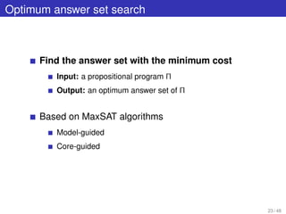
2. Optimum answer set search
Given a ground ASP program Π, find an answer set of Π
with the minimum cost
→ [Marra et al., JELIA 2014; Koponen et al., TPLP 2015]
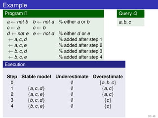
3. Cautious reasoning
Given a ground ASP program Π and a ground atom a,
check whether a is true in all answer sets of Π
→ [Arenas et al., TPLP 2003; Eiter, LPNMR 2005]
7 / 48

9. Computational tasks: complexity
Computational Normal Disjunctive
Task Programs Programs
Model
Generation NP-complete ΣP
2 -complete
Optimum
Answer Set ∆P
2 -complete ∆P
3 -complete
Search
Cautious
Reasoning coNP-complete ΠP
2 -complete
8 / 48

10. ASP syntax and semantics
Syntax:
a1 ∨ · · · ∨ an ← b1, . . . , bk , ∼ bk+1, . . . , ∼ bm
head body
Intuitive meaning:
“The head must be true whenever the body is true.”
9 / 48

11. ASP syntax and semantics
Syntax:
a1 ∨ · · · ∨ an ← b1, . . . , bk , ∼ bk+1, . . . , ∼ bm
head body
Intuitive meaning:
“The head must be true whenever the body is true.”
Definition (Stable models)
An interpretation I is a stable model (answer set) of a program
Π if I is a minimal model of ΠI, i.e., Π where the interpretation of
negative literals is fixed by I.
9 / 48

12. Example
Program Π
a | b ← c
a ← b
b ← a
c ← ∼d
d ← ∼c
Interpretation I1
a, b, c
Interpretation I2
a, b, d
10 / 48

13. Example
Program Π
a | b ← c
a ← b
b ← a
c ← ∼d
d ← ∼c
Interpretation I1
a, b, c
Reduct ΠI1
a | b ← c
a ← b
b ← a
c ← ∼d
d ← ∼c
Interpretation I2
a, b, d
10 / 48

14. Example
Program Π
a | b ← c
a ← b
b ← a
c ← ∼d
d ← ∼c
Interpretation I1
a, b, c
Reduct ΠI1
a | b ← c
a ← b
b ← a
c ← ∼d
d ← ∼c
I1 is stable
Interpretation I2
a, b, d
10 / 48

15. Example
Program Π
a | b ← c
a ← b
b ← a
c ← ∼d
d ← ∼c
Interpretation I1
a, b, c
Reduct ΠI1
a | b ← c
a ← b
b ← a
c ← ∼d
d ← ∼c
I1 is stable
Interpretation I2
a, b, d
Reduct ΠI2
a | b ← c
a ← b
b ← a
c ← ∼d
d ← ∼c
10 / 48

16. Example
Program Π
a | b ← c
a ← b
b ← a
c ← ∼d
d ← ∼c
Interpretation I1
a, b, c
Reduct ΠI1
a | b ← c
a ← b
b ← a
c ← ∼d
d ← ∼c
I1 is stable
Interpretation I2
a, b, d
Reduct ΠI2
a | b ← c
a ← b
b ← a
c ← ∼d
d ← ∼c
I2 is not stable
d is a model of ΠI2
10 / 48

17. Properties of answer sets
Supportedness: All atoms in answer set must be
supported
Example
b ← a
a ← b, ∼ c
I = {a, b} is an answer set and a and b are supported
Unfounded-free: an answer set is unfounded-free
Example
b ← a
a ← b
I = {a, b} is a supported model but it is not an answer set
11 / 48

18. ASP encoding of TSP
Example (Travelling Salesman Problem)
Input: A weighted, directed graph G = V, E, φ
A vertex s ∈ V
Goal: Find the Hamiltonian cycle of minimum weight
% Guess a cycle
in(x, y) ∨ out(x, y) ← ∀(x, y) ∈ E
% A vertex can be reached only once
← #count{1 : in(x, y) | y ∈ V} = 1 ∀x ∈ V
← #count{1 : in(x, y) | x ∈ V} = 1 y ∈ V
% All vertices must be reached
← not reached(x) ∀x ∈ V
reached(y) ← in(s, y) ∀y ∈ V
reached(y) ← reached(x), in(x, y) ∀(x, y) ∈ E
% Minimize the sum of distances
← in(x, y) [φ(x, y)] ∀(x, y) ∈ E
Guess
Check
Aux. Rules
Optimize
12 / 48

19. Outline
1 Answer Set Programming (ASP)
2 ASP computational tasks
3 Conclusion
13 / 48

20. Architecture of an ASP solver
Input pre-
processing
Numeric format
Simplifications
Controller
Model
generator
Optimum
answer set
interface
Cautious
reasoning
interface
Answer
14 / 48

21. Input preprocessing and simplifications
Preprocessing of the input program
Deletion of duplicate rules
- Even more than 80% in some benchmarks
Deterministic inferences
- Deletion of satisfied rules
Clark’s completion
- Constraints for discarding unsupported models
Simplifications
In the style of SATELITE [Eén and Biere, SAT 2005]
- Subsumption, self-subsumption, literals elimination
15 / 48

22. Model Generator
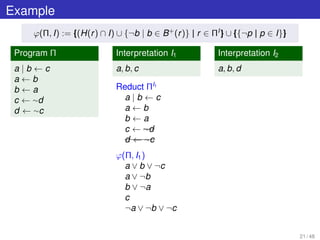
I := preprocessing()
I := propagation(I)
AnswerSet := I
I := chooseUndefinedLiteral(I)
analyzeConflict(I))
I := restoreConsistency(I)
Incoherent AnswerSet
[inconsistent]
learning
backjumping
[consistent]
[no undefined literals]
[fail]
[succeed]
16 / 48

23. Propagation
Derivation Rules
1. Unit propagation (from SAT)
2. Aggregates propagation (from Pseudo-Boolean)
3. Unfounded-free propagation (ASP specific)
17 / 48

24. Unit and Aggregate propagation
Infer a literal if it is the only one which can satisfy a rule
Example (Unit propagation)
a ← b, c.
If b and c are true then a must be true
Uses aggregates for further inferences
Example (Aggregate propagation)
← #sum{1 : d; 2 : e; 1 : f} =2
If d is true then e and f must be false
18 / 48

25. Unfounded-free propagation
All atoms in an unfounded set are inferred as false
Example (Unfounded set)
a ← b
b ← a
{a, b} is an unfounded set, thus a and b are inferred as false
19 / 48

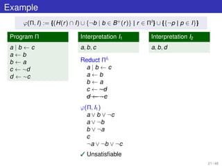
26. Unfounded-free check
HCF programs
Unfounded-free check can be done in polynomial time
Algorithm based on source pointers [Simons et al., Artif.
Intell. 2002]
non-HCF programs
Unfounded-free check is co-NP complete
Algorithm based on calls to a SAT oracle [Koch et al., Artif.
Intell. 2003]
Input: an input program Π and an interpretation I
Output: a formula ϕ such that I is unfounded-free if and only
if ϕ is unsatisfiable
20 / 48

27. Example
ϕ(Π, I) := {(H(r) ∩ I) ∪ {¬b | b ∈ B+
(r)} | r ∈ ΠI
} ∪ {{¬p | p ∈ I}}
Program Π
a | b ← c
a ← b
b ← a
c ← ∼d
d ← ∼c
Interpretation I1
a, b, c
Interpretation I2
a, b, d
21 / 48

28. Example
ϕ(Π, I) := {(H(r) ∩ I) ∪ {¬b | b ∈ B+
(r)} | r ∈ ΠI
} ∪ {{¬p | p ∈ I}}
Program Π
a | b ← c
a ← b
b ← a
c ← ∼d
d ← ∼c
Interpretation I1
a, b, c
Reduct ΠI1
a | b ← c
a ← b
b ← a
c ← ∼d
d ← ∼c
Interpretation I2
a, b, d
21 / 48

29. Example
ϕ(Π, I) := {(H(r) ∩ I) ∪ {¬b | b ∈ B+
(r)} | r ∈ ΠI
} ∪ {{¬p | p ∈ I}}
Program Π
a | b ← c
a ← b
b ← a
c ← ∼d
d ← ∼c
Interpretation I1
a, b, c
Reduct ΠI1
a | b ← c
a ← b
b ← a
c ← ∼d
d ← ∼c
ϕ(Π, I1)
a ∨ b ∨ ¬c
a ∨ ¬b
b ∨ ¬a
c
¬a ∨ ¬b ∨ ¬c
Interpretation I2
a, b, d
21 / 48

30. Example
ϕ(Π, I) := {(H(r) ∩ I) ∪ {¬b | b ∈ B+
(r)} | r ∈ ΠI
} ∪ {{¬p | p ∈ I}}
Program Π
a | b ← c
a ← b
b ← a
c ← ∼d
d ← ∼c
Interpretation I1
a, b, c
Reduct ΠI1
a | b ← c
a ← b
b ← a
c ← ∼d
d ← ∼c
ϕ(Π, I1)
a ∨ b ∨ ¬c
a ∨ ¬b
b ∨ ¬a
c
¬a ∨ ¬b ∨ ¬c
Unsatisfiable
Interpretation I2
a, b, d
21 / 48

31. Example
ϕ(Π, I) := {(H(r) ∩ I) ∪ {¬b | b ∈ B+
(r)} | r ∈ ΠI
} ∪ {{¬p | p ∈ I}}
Program Π
a | b ← c
a ← b
b ← a
c ← ∼d
d ← ∼c
Interpretation I1
a, b, c
Reduct ΠI1
a | b ← c
a ← b
b ← a
c ← ∼d
d ← ∼c
ϕ(Π, I1)
a ∨ b ∨ ¬c
a ∨ ¬b
b ∨ ¬a
c
¬a ∨ ¬b ∨ ¬c
Unsatisfiable
Interpretation I2
a, b, d
Reduct ΠI2
a | b ← c
a ← b
b ← a
c ← ∼d
d ← ∼c
21 / 48

32. Example
ϕ(Π, I) := {(H(r) ∩ I) ∪ {¬b | b ∈ B+
(r)} | r ∈ ΠI
} ∪ {{¬p | p ∈ I}}
Program Π
a | b ← c
a ← b
b ← a
c ← ∼d
d ← ∼c
Interpretation I1
a, b, c
Reduct ΠI1
a | b ← c
a ← b
b ← a
c ← ∼d
d ← ∼c
ϕ(Π, I1)
a ∨ b ∨ ¬c
a ∨ ¬b
b ∨ ¬a
c
¬a ∨ ¬b ∨ ¬c
Unsatisfiable
Interpretation I2
a, b, d
Reduct ΠI2
a | b ← c
a ← b
b ← a
c ← ∼d
d ← ∼c
ϕ(Π, I2)
a ∨ ¬b
b ∨ ¬a
d
¬a ∨ ¬b ∨ ¬d
21 / 48

33. Example
ϕ(Π, I) := {(H(r) ∩ I) ∪ {¬b | b ∈ B+
(r)} | r ∈ ΠI
} ∪ {{¬p | p ∈ I}}
Program Π
a | b ← c
a ← b
b ← a
c ← ∼d
d ← ∼c
Interpretation I1
a, b, c
Reduct ΠI1
a | b ← c
a ← b
b ← a
c ← ∼d
d ← ∼c
ϕ(Π, I1)
a ∨ b ∨ ¬c
a ∨ ¬b
b ∨ ¬a
c
¬a ∨ ¬b ∨ ¬c
Unsatisfiable
Interpretation I2
a, b, d
Reduct ΠI2
a | b ← c
a ← b
b ← a
c ← ∼d
d ← ∼c
ϕ(Π, I2)
a ∨ ¬b
b ∨ ¬a
d
¬a ∨ ¬b ∨ ¬d
{d} is a model
21 / 48

34. Heuristics and learning
Learning
Detect the reason of a conflict
Learn constraints using 1-UIP schema
Deletion Policy
Exponentially many constraints → forget something
Less “useful” constraints are removed
Search Restarts
Avoid unfruitful branches by restarting the search
Based on some heuristic sequence
Branching Heuristics
Look back MINISAT heuristic
22 / 48

35. Optimum answer set search
Find the answer set with the minimum cost
Input: a propositional program Π
Output: an optimum answer set of Π
Based on MaxSAT algorithms
Model-guided
Core-guided
23 / 48

36. Optimum answer set search
Model-guided algorithms: OPT, BASIC and MGD
+ Easy to implement
+ Work well on particular domains
+ Produce feasible solutions during the search
- Poor performances on industrial instances
Core-guided algorithms: PMRES and OLL
+ Good performances on industrial instances
- Do not produce feasible solutions (in general)
- The implementation is usually nontrivial
24 / 48

37. Model-guided algorithms
I need a solution! Give me any answer set
remove weak constraints from the program
model generator
add violated weak constraints to the program
update upper bound
Optimum found
[coherent]
[incoherent]
25 / 48

38. Core-guided algorithms
I feel lucky! Try to satisfy all weak constraints
consider weak constraints as hard
model generator
analyze unsatisfiable core
update lower bound
Optimum found
[incoherent]
[coherent]
26 / 48

39. Stratification
1. Generic technique
→ can be applied to PMRES, OLL, . . .
2. Force the ASP solver to concentrate on weak constraints
with higher weights
27 / 48

40. Stratification
wmax := +∞
wmax := max{wi | ri ∈ weak(Π) ∧ wi wmax}
consider weak constraints in {ri | wi ≥ wmax} as hard
model generator
analyze unsatisfiable core
Optimum found
[incoherent]
[coherent]
[wmax = 0]
[wmax 0]
28 / 48

41. Cautious reasoning
Formally, an atom a is a cautious consequence of a
program Π if a belongs to all stable models of Π
Compute cautious consequences
Input: a propositional program Π
Output: all cautious consequences of Π
29 / 48

42. Cautious reasoning: algorithms
Enumeration of models (DLV)
Overestimate reduction (CLASP)
Iterative coherence testing (WASP)
30 / 48

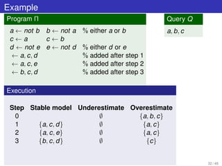
43. Cautious reasoning by enumeration of models
Answers := ∅; Candidates := Query
model generator
Answers := Candidates
Answers
Candidates := Candidates ∩ AnswerSet
Π := Π ∪ Constraint(AnswerSet)
[coherent]
[incoherent]
31 / 48

44. Example
32 / 48
Query Q
a, b, c
Program Π
a ← not b b ← not a % either a or b
c ← a c ← b
d ← not e e ← not d % either d or e
Execution
Step Stable model Underestimate Overestimate
0 ∅ {a, b, c}

45. Example
32 / 48
Query Q
a, b, c
Program Π
a ← not b b ← not a % either a or b
c ← a c ← b
d ← not e e ← not d % either d or e
← a, c, d % added after step 1
Execution
Step Stable model Underestimate Overestimate
0 ∅ {a, b, c}
1 {a, c, d} ∅ {a, c}

46. Example
32 / 48
Query Q
a, b, c
Program Π
a ← not b b ← not a % either a or b
c ← a c ← b
d ← not e e ← not d % either d or e
← a, c, d % added after step 1
← a, c, e % added after step 2
Execution
Step Stable model Underestimate Overestimate
0 ∅ {a, b, c}
1 {a, c, d} ∅ {a, c}
2 {a, c, e} ∅ {a, c}

47. Example
32 / 48
Query Q
a, b, c
Program Π
a ← not b b ← not a % either a or b
c ← a c ← b
d ← not e e ← not d % either d or e
← a, c, d % added after step 1
← a, c, e % added after step 2
← b, c, d % added after step 3
Execution
Step Stable model Underestimate Overestimate
0 ∅ {a, b, c}
1 {a, c, d} ∅ {a, c}
2 {a, c, e} ∅ {a, c}
3 {b, c, d} ∅ {c}

48. Example
32 / 48
Query Q
a, b, c
Program Π
a ← not b b ← not a % either a or b
c ← a c ← b
d ← not e e ← not d % either d or e
← a, c, d % added after step 1
← a, c, e % added after step 2
← b, c, d % added after step 3
← b, c, e % added after step 4
Execution
Step Stable model Underestimate Overestimate
0 ∅ {a, b, c}
1 {a, c, d} ∅ {a, c}
2 {a, c, e} ∅ {a, c}
3 {b, c, d} ∅ {c}
4 {b, c, e} ∅ {c}

49. Example
32 / 48
Query Q
a, b, c
Program Π
a ← not b b ← not a % either a or b
c ← a c ← b
d ← not e e ← not d % either d or e
← a, c, d % added after step 1
← a, c, e % added after step 2
← b, c, d % added after step 3
← b, c, e % added after step 4
Execution
Step Stable model Underestimate Overestimate
0 ∅ {a, b, c}
1 {a, c, d} ∅ {a, c}
2 {a, c, e} ∅ {a, c}
3 {b, c, d} ∅ {c}
4 {b, c, e} ∅ {c}
5 Incoherent {c} {c}

50. Example
32 / 48
Query Q
a, b, c
Program Π
a ← not b b ← not a % either a or b
c ← a c ← b
d ← not e e ← not d % either d or e
← a, c, d % added after step 1
← a, c, e % added after step 2
← b, c, d % added after step 3
← b, c, e % added after step 4
Execution
Step Stable model Underestimate Overestimate
0 ∅ {a, b, c}
1 {a, c, d} ∅ {a, c}
2 {a, c, e} ∅ {a, c}
3 {b, c, d} ∅ {c}
4 {b, c, e} ∅ {c}
5 Incoherent {c} {c}

51. Cautious reasoning by enumeration of models
Cautious reasoning by enumeration of models
+ Easy to be implemented
- Redundant computation
- Poor performances
- Does not produce answers during the computation
33 / 48

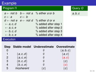
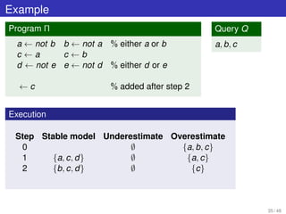
52. Cautious reasoning by overestimate reduction
Answers := ∅; Candidates := Query
model generator
Answers := Candidates
Answers
Candidates := Candidates ∩ AnswerSet
Π := Π ∪ Constraint(Candidates)
[coherent]
[incoherent]
34 / 48

53. Example
35 / 48
Query Q
a, b, c
Program Π
a ← not b b ← not a % either a or b
c ← a c ← b
d ← not e e ← not d % either d or e
Execution
Step Stable model Underestimate Overestimate
0 ∅ {a, b, c}

54. Example
35 / 48
Query Q
a, b, c
Program Π
a ← not b b ← not a % either a or b
c ← a c ← b
d ← not e e ← not d % either d or e
← a, c % added after step 1
Execution
Step Stable model Underestimate Overestimate
0 ∅ {a, b, c}
1 {a, c, d} ∅ {a, c}

55. Example
35 / 48
Query Q
a, b, c
Program Π
a ← not b b ← not a % either a or b
c ← a c ← b
d ← not e e ← not d % either d or e
← c % added after step 2
Execution
Step Stable model Underestimate Overestimate
0 ∅ {a, b, c}
1 {a, c, d} ∅ {a, c}
2 {b, c, d} ∅ {c}

56. Example
35 / 48
Query Q
a, b, c
Program Π
a ← not b b ← not a % either a or b
c ← a c ← b
d ← not e e ← not d % either d or e
← c % added after step 2
Execution
Step Stable model Underestimate Overestimate
0 ∅ {a, b, c}
1 {a, c, d} ∅ {a, c}
2 {b, c, d} ∅ {c}
3 Incoherent {c} {c}

57. Example
35 / 48
Query Q
a, b, c
Program Π
a ← not b b ← not a % either a or b
c ← a c ← b
d ← not e e ← not d % either d or e
← c % added after step 2
Execution
Step Stable model Underestimate Overestimate
0 ∅ {a, b, c}
1 {a, c, d} ∅ {a, c}
2 {b, c, d} ∅ {c}
3 Incoherent {c} {c}

58. Cautious reasoning by overestimate reduction
Cautious reasoning by overestimate reduction
+ Force each stable model to remove at least one candidate
from the overestimate
- Does not produce answers during the computation
36 / 48

59. Cautious reasoning by iterative coherence testing
Answers := ∅; Candidates := Query
a := OneOf(Candidates Answers)
model generator on Π ∪ {← a}
Answers
Candidates := Candidates ∩ AnswerSet
Answers := Answers ∪ {a}
[Answers = Candidates]
[coherent]
[incoherent]
37 / 48

60. Example
38 / 48
Query Q
a, b, c
Program Π
a ← not b b ← not a % either a or b
c ← a c ← b
d ← not e e ← not d % either d or e
Execution
Step OneOf Stable model Underestimate Overestimate
0 ∅ {a, b, c}

61. Example
38 / 48
Query Q
a, b, c
Program Π
a ← not b b ← not a % either a or b
c ← a c ← b
d ← not e e ← not d % either d or e
Execution
Step OneOf Stable model Underestimate Overestimate
0 ∅ {a, b, c}
1 {a, c, d} ∅ {a, c}

62. Example
38 / 48
Query Q
a, b, c
Program Π
a ← not b b ← not a % either a or b
c ← a c ← b
d ← not e e ← not d % either d or e
Execution
Step OneOf Stable model Underestimate Overestimate
0 ∅ {a, b, c}
1 {a, c, d} ∅ {a, c}
2 c Incoherent {c} {a, c}

63. Example
38 / 48
Query Q
a, b, c
Program Π
a ← not b b ← not a % either a or b
c ← a c ← b
d ← not e e ← not d % either d or e
Execution
Step OneOf Stable model Underestimate Overestimate
0 ∅ {a, b, c}
1 {a, c, d} ∅ {a, c}
2 c Incoherent {c} {a, c}
3 a {b, c, d} {c} {c}

64. Example
38 / 48
Query Q
a, b, c
Program Π
a ← not b b ← not a % either a or b
c ← a c ← b
d ← not e e ← not d % either d or e
Execution
Step OneOf Stable model Underestimate Overestimate
0 ∅ {a, b, c}
1 {a, c, d} ∅ {a, c}
2 c Incoherent {c} {a, c}
3 a {b, c, d} {c} {c}

65. Cautious reasoning by iterative coherence testing
Cautious reasoning by iterative coherence testing
+ Produce sound answers during the computation
+ Good performances
- The function OneOf is crucial for the performances
39 / 48

66. Anytime variants
Often termination cannot be achieved in reasonable time
Anytime algorithms are crucial for such cases to produce
some sound answers
It is important to be anytime
The problem is ΠP
2 -complete
⇓
There are a few instances that are ΠP
2 -hard
40 / 48

67. Anytime variants
Often termination cannot be achieved in reasonable time
Anytime algorithms are crucial for such cases to produce
some sound answers
It is important to be anytime
The problem is ΠP
2 -complete
⇓
There are a few instances that are ΠP
2 -hard
Good news!
Any algorithm for cautious reasoning can be anytime
40 / 48

68. Anytime variants
Often termination cannot be achieved in reasonable time
Anytime algorithms are crucial for such cases to produce
some sound answers
It is important to be anytime
The problem is ΠP
2 -complete
⇓
There are a few instances that are ΠP
2 -hard
Good news!
Any algorithm for cautious reasoning can be anytime
Just check for new sound answers after each restart
40 / 48

69. Cautious reasoning
0
0%25%50%75%100%
10 seconds 1 minute 2 minutes 5 minutes Up to timeout
OvRed
OvRed*
ICT*
OvRed
OvRed*
ICT*
OvRed
OvRed*
ICT*
0 20 40 60 80 100
MCS
CQA
SBB
41 / 48

70. State of the art
42 / 48

71. Outline
1 Answer Set Programming (ASP)
2 ASP computational tasks
3 Conclusion
43 / 48

72. Conclusion (1)
ASP solving require solutions for several computational
tasks
Model generation
Preprocessing, CDCL-like algorithm
Optimum answer set search
Model and core-guided algorithms
Cautious reasoning
Framework of anytime algorithms
44 / 48

73. Conclusion (2)
ASP systems
CLASP (http://potassco.sourceforge.net/)
CMODELS (http:
//www.cs.utexas.edu/users/tag/cmodels/)
DLV (http://www.dlvsystem.com/)
IDP
(https://dtai.cs.kuleuven.be/software/idp)
LP2SAT (http://research.ics.aalto.fi/
software/asp/download/)
MEASP
(https://www.mat.unical.it/ricca/me-asp/)
WASP (http://alviano.github.io/wasp/)
45 / 48

74. Thank you!
46 / 48

75. Bibliography (1)
[Arenas et al., TPLP 2003] M. Arenas, L. E. Bertossi, J. Chomicki. Answer
sets for consistent query answering in inconsis-
tent databases. TPLP 3(4-5): 393-424 (2003).
[Balduccini et al., LPNMR 2001] M. Balduccini, M. Gelfond, R. Watson, M.
Nogueira. The USA-Advisor: A Case Study in
Answer Set Planning. LPNMR 2001: 439-442.
[Eén and Biere, SAT 2005] N. Eén, A. Biere. Effective Preprocessing in SAT
Through Variable and Clause Elimination. SAT
2005: 61-75.
[Eiter, LPNMR 2005] T. Eiter. Data Integration and Answer Set Pro-
gramming. LPNMR 2005: 13-25.
[Gebser et al., TPLP 2011] M. Gebser, T. Schaub, S. Thiele, P. Veber. De-
tecting inconsistencies in large biological net-
works with answer set programming. TPLP 11(2-
3): 323-360 (2011).
47 / 48

76. Bibliography (2)
[Koch et al., Artif. Intell. 2003] C. Koch, N. Leone, G. Pfeifer. Enhancing
disjunctive logic programming systems by SAT
checkers. Artif. Intell. 151(1-2): 177-212 (2003).
[Koponen et al., TPLP 2015] L. Koponen, E. Oikarinen, T. Janhunen, L. Säilä.
Optimizing phylogenetic supertrees using an-
swer set programming. TPLP 15(4-5): 604-619
(2015).
[Marra et al., JELIA 2014] G. Marra, F. Ricca, G. Terracina, D. Ursino. Ex-
ploiting Answer Set Programming for Handling
Information Diffusion in a Multi-Social-Network
Scenario. JELIA 2014: 618-627.
[Simons et al., Artif. Intell. 2002] P. Simons, I. Niemelä, T. Soininen. Extending
and implementing the stable model semantics.
Artif. Intell. 138(1-2): 181-234 (2002).
48 / 48