jelia2002-tutorial.ppt answer set programming

Answer Set Programming
Basics, Knowledge Representation,
Systems, and Computational Issues
Gerald Pfeifer
TU Wien
http://www.dbai.tuwien.ac.at/~pfeifer/

Roadmap
 Setting
 Syntax and Semantics
 Language by Examples
 Guess&Check Paradigm
 Optimization / Weak Constraints
 Implementations
 [ Computational Issues ]
 [ Bibliography ]

Keywords
 „Solving problems in a fast and declarative way“
 Knowledge Representation
 Disjunctive Databases / Datalog
 Disjunctive Logic Programming
 Logic (stable models, answer sets)

Applications
 Knowledge Representation
 Incomplete Information
 Artificial Intelligence
 Diagnosis
 Planning
 Complex problems not easily and/or polynomially
translatable to SAT
 Emerging Applications Areas
 Knowledge Management
 Information Integration

Roots  Declarative
Programming
 Algorithm = Logic + Control (Kowalski, 1979)
 First-order logic as a programming language
 Expectations, hopes
 - easy programming, fast prototyping
 - handle on program verification
 - advancement of software engineering

Enter ASP: Advantages
 Sound theoretical foundation
- Model Theory
 Nice formal properties (clear semantics)
 Real Declarativeness
 Ordering of Rules/Goals is Immaterial!
 Termination always guaranteed
 High expressive power

ASP: Drawbacks
 Computing Answer Sets is rather hard:
 NP ... without (full) disjunction,
 ... with full disjunction,
 a bit higher, when we use optimization.
 Few solid and efficient implementations.
 ...but this has started to change:
DLV, Smodels, ASSAT, ...
P
2
P
2


Syntax and Semantics
Possibly boring, but needed....
getFunLater :- persistNow.
[Nicola Leone]

ASP: The Language
Classic Logic Programming extended with
 disjunction
 default negation
 strong negation
 integrity constraints
 weak constraints
 integers, arithmetic, and comparison builtins
 no „full“ function symbols

ASP Syntax
Rules: a1  …  an :-b1, …, bk , not bk+1 , …, not bm.
Constraints: :- b1 , …, bk , not bk+1 , …, not bm.
Program: A finite set P of rules and constraints.
 as and bs are atoms or strongly negated atoms (-p),
 variables are allowed in arguments of atoms.
 „Read“ rules from right to left!
boy(X) v girl(X) :- child(X).
mother(Par,Child) v father(Par,Child) :-parent(Par,Child).

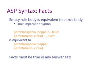
ASP Syntax: Facts
Empty rule body is equivalent to a true body.
 Omit implication symbol.
parent(eugenio, peppe) :- „true“.
parent(mario, ciccio) :- „true“.
is equivalent to.
parent(eugenio, peppe).
parent(mario, ciccio).
Facts must be true in any answer set!

Semantics: Rules
a1  …  an :- b1, …, bk , not bk+1 , …, not bm.
 If all b1,…,bk are true and all bk+1,…,bm are false,
then at least one among a1,…,an is true.
interestedInTutorial(you) v curious(you)
:- attendsTutorial(you).
attendsTutorial(you).
 Two (minimal) models, encoding plausible scenarios:
 M1: {attendsTutorial(you), interestedInTutorial(you)}
 M2: {attendsTutorial(you), curious(you)}

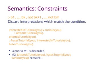
Semantics: Constraints
:- b1 , …, bk , not bk+1 , …, not bm
Discard interpretations which match the condition.
interestedInTutorial(you) v curious(you)
:- attendsTutorial(you).
attendsTutorial(you).
:- hatesTutorial(you), interestedInTutorial(you).
hatesTutorial(you).
 Scenario M1 is discarded.
 M2‘ {attendsTutorial(you), hatesTutorial(you),
curious(you)} remains.

Semantics: Program Instantiation
Herbrand Universe, UP: set of constants occurring in program P
Herbrand Base, BP: set of ground atoms constructible from UP and Predicates
Ground instance of a rule R: replace all variables in R by constants in UP
Instantiation ground(P) of a program P: set of all ground instances of all rules
Example: interestedInTutorial(X) v curious(X) :- attendsTutorial(X).
attendsTutorial(peppe).
attendsTutorial(tina).
UP={ peppe, tina }
interestedInTutorial(peppe) v curious(peppe) :- attendsTutorial(peppe).
interestedInTutorial(tina) v curious(tina) :- attendsTutorial(tina).
attendsTutorial(peppe). attendsTutorial(tina).
A program with variables is a shorthand for its ground instantiation!

Semantics: Interpretation I of
P
Consistent set of (classical) atoms of P, where
 an atom q is true in I if q belongs to I;
otherwise it is false.
 a literal not q is true in I if q is false in I;
otherwise it is false.
 An interpretation I is closed under P if, for
every R in P, the head of R is true in I,
whenever the body of R is true in I.
 Bodies of constraint must be false!

Semantics: Positive
Programs
 Assume programs are ground (replace
P by ground(P)) and positive (not-free).
 I is an answer set for a positive
program P if it is a minimal set
(wrt. set inclusion) closed under P.
 Uhh???

Semantics: Positive Programs – Example 1
interestedInTutorial(peppe) v curious(peppe) :-
interestedInTutorial(tina) v curious(tina) :- attendsTutorial(tina).
attendsTutorial(tina).
I1 = { attendsTutorial(peppe) } (not closed)
I2 = { attendsTutorial(peppe), curious(peppe), attendsTutorial(tina),
interestedInTutorial(tina), curious(tina) } (closed, non minimal)
I3 = {attendsTutorial(peppe), curious(peppe), attendsTutorial(tina),
interestedInTutorial(tina) } (answer set)
I4={ attendsTutorial(peppe), interestedInTutorial(peppe),
attendsTutorial(tina), interestedInTutorial(tina) } (answer set)
I5 = {attendsTutorial(peppe), curious(peppe), attendsTutorial(tina) ,
curious(tina) } (answer set)
I6={attendsTutorial(peppe), interestedInTutorial(peppe),
attendsTutorial(tina) , curious(tina) } (answer set)

Semantics: Positive Programs – Example 2
Let us add:
:- hatesTutorial(peppe), interestedInTutorial(peppe).
hatesTutorial(peppe).
(Same interpretations as before + {hatesTutorial(peppe)} )
I1 = { attendsTutorial(peppe), hatesTutorial(peppe) } (not closed)
I2 = {attends...(peppe), curious(peppe), attends...(tina), interested...(tina),
curious(tina), hatesTutorial(peppe) } (closed, not minimal)
interestedInTutorial(tina), hatesTutorial(peppe) } (answer set)
I4={attendsTutorial(peppe), interested...(peppe), attendsTutorial(tina),
interested...(tina), hatesTutorial(peppe) } (not closed!!)
curious(tina), hatesTutorial(peppe) } (answer set)
I6={attendsTutorial(peppe), interestedInTutorial(peppe),
attendsTutorial(tina), curious(tina), hatesTutorial(peppe) } (not closed!!)

Semantics: Programs with Negation
The Gelfond-Lifschitz reduct of a program P wrt. An interpretation I is the positive
program PI
, obtained from P by
 deleting all rules with a negative literal false in I;
 deleting the negative literals from the bodies of the remaining rules.
An Answer Set of a program P is an interpretation I such that I is an answer set of
PI
.
Answer Sets are also called Stable Models.

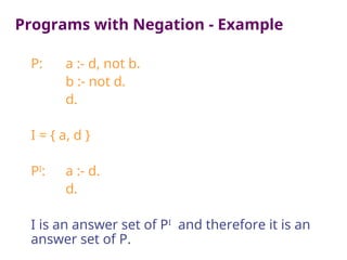
Programs with Negation - Example
P: a :- d, not b.
b :- not d.
d.
I = { a, d }
PI
: a :- d.
d.
I is an answer set of PI
and therefore it is an
answer set of P.

Derivation
Relations can be expressed intentionally
through logical rules.
Parent (a, b).
Parent (b, c).
Grandparent (X, Y) :- Parent (X,Z), Parent (Z,Y).
M = { GrandParent (a, c), Parent (a, b), Parent (b, c) }

Recursion: Ancestor
To define the relation of arbitrary
ancestors rather than grandparents, we
make use of recursion:
 ancestor(A,B) :- parent(A,B).
ancestor(A,C) :- ancestor(A,B), ancestor(B,C).
An equivalent representation is
ancestor(A,C) :- ancestor(A,B), parent(B,C).

ASP offers Full
Declarativeness!
The order of rules and of goals is immaterial:
ancestor(A,C) :- ancestor(A,B), ancestor(B,C).
is fully equivalent to
 ancestor(A,C) :- ancestor(A,B), ancestor(B,C).
ancestor(A,B) :- parent(A,B).
and also to
 ancestor(A,C) :- ancestor(B,C), ancestor(A,B).
ancestor(A,B) :- parent(A,B).
No infinite loop!

Recursion: Reachability
Input: A set of direct connections between
cities represented by facts of the form
connected(_,_).
Problem: For each city C, find the cities
which are reachable from C.
reaches(A,O) :- connected(A,O).
reaches(A,Inter) :- reaches(A,Inter), connected(Inter,C).

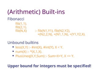
(Arithmetic) Built-ins
Fibonacci
fib(1,1).
fib(2,1).
fib(N,X) :- fib(N1,Y1), fib(N2,Y2),
+(N2,2,N), +(N1,1,N), +(Y1,Y2,X).
Unbound builtins
 less(X,Y) :- #int(X), #int(Y), X < Y.
 num(X) :- *(X,1,X).
 PlusUneq(X,Y,Sum) :- Sum=X+Y, X <> Y.
Upper bound for integers must be specified!

Default Negation: „not“
Often, it is desirable to express negation in
the following sense: “If we do not have
evidence that X holds, conclude Y.”
Example: an agent could act according to the
following rule:
“At a railroad crossing, cross the rails if no train
approaches.”
cross(A) :- crossing(A), not train_approaches(A).

Strong (or True) Negation
However, in our example default negation is
not really acceptable:
 A train might approach, though we don‘t have
evidence for it (e.g. we do not hear the train).
 It would be desirable to definitely know that no
train approaches.
This concept is called strong (or true) negation:
cross(A) :- crossing(A), -train_approaches(A).
 Can lead to inconsistencies!
{a, -a}

Disjunction 1/2
Programs with disjunction can have
more than one model.

Disjunction 2/2
 is minimal:
a v b v c  { a }, { b }, { c }
 actually subset minimal:
a v b.
a v c.  {a}, {b,c}
 but not exclusive:
a v b.
a v c.  {a,b}, {a,c}, {b,c}
b v c.

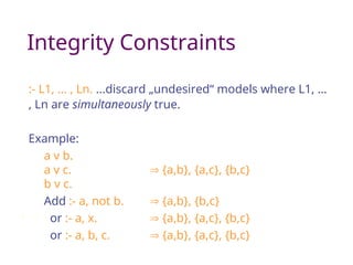
Integrity Constraints
:- L1, … , Ln. ...discard „undesired“ models where L1, …
, Ln are simultaneously true.
Example:
a v b.
a v c.  {a,b}, {a,c}, {b,c}
b v c.
Add :- a, not b.  {a,b}, {b,c}
or :- a, x.  {a,b}, {a,c}, {b,c}
or :- a, b, c.  {a,b}, {a,c}, {b,c}
.

Aggregate Functions
 Vary greatly from system to system!
 DLV: #count, #min, #max, #sum, #avg
 Compute the project cost by summing up the
salaries of all the employees working in the
project.
 globalCost(X) :-
X= #sum ( S : salary(E,S),
employee(E) ).

The Guess&Check Paradigm
Idea: encode a search problem PROB by an ASP
program P.
The answer sets of P correspond one-to-one to
the solutions of PROB.
Methodology:
 Generate-and-test programming:
 Generate possible structures.
 Weed out unwanted solutions by adding constraints.
 Separate data from program.

Guess&Check (ASP)
 Disjunctive rules “guess” solution candidates.
 Integrity constraints check their admissibility.
From another perspective:
 The disjunctive rule defines the search space.
 Integrity constraints prune illegal branches.

3-colorability
Input: a Map represented by state(_) and border(_,_).
Problem: assign one color out of 3 colors to each state such
that two neighbouring states always have different colors.
Solution:
col(X,red) v col(X,green) v col(X,blue) :-state(X). } Guess
:- border(X,Y), col(X,C), col(Y,C). } Check

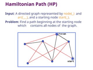
Hamiltonian Path (HP)
Input: A directed graph represented by node(_) and
arc(_,_), and a starting node start(_).
Problem: Find a path beginning at the starting node
which contains all nodes of the graph.

Hamiltonian Path - Encoding
inPath(X,Y) v outPath(X,Y) :- arc(X,Y). Guess
:- inPath(X,Y), inPath(X,Y1), Y <> Y1.
:- inPath(X,Y), inPath(X1,Y), X <> X1. Check
:- node(X), not reached(X).
reached(X) :- start(X). Auxiliary Predicate
reached(X) :- reached(Y), inPath(Y,X).

Strategic Companies
Input: There are various products, each one is produce
by several companies.
Problem: We now have to sell some companies.
What are the minimal sets of strategic companies, such
that all products can still be produced?
A company also belong to the set, if all its controlling
companies belong to it.
strategic(Y) v strategic(Z) :- produced_by(X, Y, Z). Guess
strategic(W) :- controlled_by(W, X, Y, Z), Constraints
strategic(X), strategic(Y), strategic(Z).

Strategic Companies -
Example
pasta
wine
tomatoes
barilla
frutto
saiwa
budweiser
heineken
panino bread
beer
barilla
frutto
saiwa
budweiser
heineken

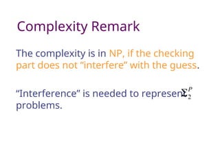
Complexity Remark
The complexity is in NP, if the checking
part does not “interfere” with the guess.
“Interference” is needed to represent
problems.
P
2


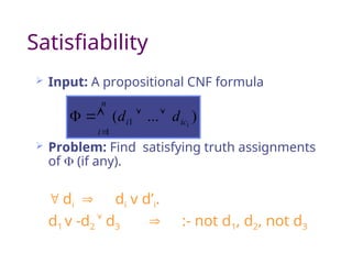
Satisfiability
 Input: A propositional CNF formula
 Problem: Find satisfying truth assignments
of  (if any).
 di  di v d’i.
d1 v -d2  d3  :- not d1, d2, not d3
)
...
( 1
1
i
ic
i
n
i
d
d 


 

Planning - Blocksworld
Objects: Some blocks and a table.
Fluent on(B, L, T): Exactly one block may be on
another block, and arbitrary many blocks may be on
the table. Every block must be on something.
Action move(B, L, T): Move a block from one location
to another. The block must be clear and the goal
location must be clear (unless it is the table).
Time: finite number of timeslots. An action is carried
out between two timeslots. Only one action at a
time.

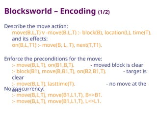
Blocksworld – Encoding (1/2)
Describe the move action:
move(B,L,T) v -move(B,L,T) :- block(B), location(L), time(T).
and its effects:
on(B,L,T1) :- move(B, L, T), next(T,T1).
Enforce the preconditions for the move:
:- move(B,L,T), on(B1,B,T). - moved block is clear
:- block(B1), move(B,B1,T), on(B2,B1,T). - target is
clear
:- move(B,L,T), lasttime(T). - no move at the
end
No concurrency:
:- move(B,L,T), move(B1,L1,T), B<>B1.
:- move(B,L,T), move(B1,L1,T), L<>L1.

Blocksworld – Encoding (2/2)
Inertia:
on(B,L,T1) :- on(B,L,T), next(T,T1), not -on(B,L,T1).
-on(B,L,T1) :- -on(B,L,T), next(T,T1), not on(B,L,T1).
A block cannot be at two locations or on itself:
- on(B,L1,T), on(B,L,T), L<>L1.
:- on(B,B,T).
Background Knowledge (time and objects):
time(T) :- #int(T). lasttime(#maxint).
next(T,T1) :- #succ(T,T1).
location(table). location(L) :- block(L).

Blocksworld - Sussman
anomaly
c
a
b
b
a
c
initial: goal:
Define blocks and the initial and goal situations:
block(a). block(b). block(c).
on(a,table,0). on(b,table,0). on(c,a,0).
on(a,table,#maxint), on(b,a,#maxint), on(c,b,#maxint) ?
The number of timeslots is given when invoking DLV:
$ dlv blocksworld sussman -N=3 -pfilter=move
{move(c,table,0), move(b,a,1), move(c,b,2)}

Optimization / Weak
Constraints
Express desiderata - constraints which should
possibly be satisfied, like Soft Constraints in CSP.
:~ B.
 Avoid B if possible.
Weak constraints can be weighted and prioritized:
:~ B. [w:p]
 higher weights/priorities -> higher importance
A useful tool to encode optimization problems.

Weak Constraints: Semantics
Rules(P): set of the rules (facts, strong constraints)
WC(P): weak constraints of P
Programs without priorities in WC(P):
 Answer sets of Rules(P) minimize the sum of the weights
of the violated constraints in WC(P).
 Weight = „Penalty“ or „Cost“.
Programs with priorities:
 first, minimize the sum of the weights of the violated
constraints in the highest priority level;
 Then, minimize the sum of the weights of the violated
constraints in the next lower level, etc.

Exams Scheduling
1. Assign course exams to time slots avoiding
overlapping of exams of courses with common
students
assign(X,time1) v ... v assign(X,time5) :- course(X).
:- assign(X,Time), assign(Y,Time), commonStuds(X,Y,N), N>0.
2. If overlapping is unavoidable, then reduce it “As
Much As Possible” – find an approximate
solution:
:~ assign(X,S), assign(Y,S), commonStudents(X,Y,N). [N:]
Scenarios that minimize the total number of “lost”
exams are preferred.

Team Building
(Prioritized Constraints)
Divide employees in two project groups p1 and p2.
A) Skills of group members should be different.
B) No married couples should be in the same group.
C) Members of a group should possibly know each other.
Plus: A) is more important than B) and C).
assign(X,proj1) v assign(X,proj2) :- employee(X).
:~ assign(X,P), assign(Y,P), same_skill(X,Y). [:2]
:~ assign(X,P), assign(Y,P), married(X,Y). [:1]
:~ assign(X,P), assign(Y,P), X<>Y, not know(X,Y). [:1]

Guess/Check/Optimize (GCO)
Programming
Generalization of Guess and Check paradigm.
Programs consists of 3 modules:
[Guessing Part] defines the search space;
[Checking Part] checks solution admissibility;
[Optimizing Part] specifies preference criterion
(by means of weak constraints).
Guideline: develop encoding incrementally!

Example – Traveling Salesperson
Hamiltonian Path
inPath(X,Y) v outPath(X,Y) :- arc(X,Y,Cost). Guess
:- inPath(X,Y), inPath(X,Y1), Y <> Y1.
:- inPath(X,Y), inPath(X1,Y), X <> X1. Check
reached(X) :- start(X). Auxiliary Predicate
reached(X) :- reached(Y), inPath(Y,X).
+ Optimization
:~ inPath(X,Y), arc(X,Y,Cost). [Cost:] Optimize

Minimum Spanning Tree
Given a weighted graph by means of edge(Node1,Node2,Cost)
and node(N), compute a tree that starts at a root node, spans
that graph, and has minimum cost.
% Guess the edges that are part of the tree.
inTree(X,Y)  outTree(X,Y) :- edge(X,Y,C). Guess
% Check that we are really dealing with a tree...
:- root(X), inTree(_,X,C).
:- inTree(X,Y), inTree(X1,Y), X <> X1.
% ...and that the tree is connected. Check
% Minimize the cost of the tree.
:~ inTree(X,Y), edge(X,Y,C). [C:] Optimize
reached(X) :- root(X). Auxiliary Predicate
reached(X) :- reached(Y), inTree(Y,X).

DLV:
System Architecture
Diagnosis
Frontend
Filtering
Model
Checker
Model
Generator
Intelligent
Grounding
Inheritance
Frontend
Brave/Cautious
Frontend
SQL3
Frontend
User Interface
Output
Ground
Program
File
System
Ground
Program
Relational
Database
ODBC

DLV: Frontends
 (Model-based) Diagnosis
 Planning
 Inheritance
 SQL3
 External Frontends (Meta-Interpreter,...)

Smodels/GnT
 Smodels is the most widely used system
for v-free programs.
 Uses a parser/grounder called Lparse.
 also used by other system (ASSAT,...)
 GnT extends Smodels by disjunction.
 rewriting + nested calls to Smodels for answer
set checking.
 Powerful constructs for representing
cardinality and weight constraints:
 3 { f(X) : something(X,Y) } 5 :- ... .

Other ASP Systems
Most systems do not support disjunction!
 ASSAT (v-free programs, rewriting to SAT)
 Cmodels (v-free, tight programs, rewriting to SAT)
 NoMoRe (v-free programs, graph-colorings)
 Dislop (model elimination, hyper-tableau calculi)
 DeReS (Default Logic)
 CCALC (acyclic V-free programs, rewriting to SAT)
 XSB (well-founded semantics)
 aspps (logic of propositional schemes)
 QUIP(based on QBF evaluators)
 SLG (Meta-Interpreter over prolog systems)
 DisLog

Availability
 http://www.dlvsystem.com
 http://www.tcs.hut.fi/Software/smodels/
 http://assat.cs.ust.hk/
 http://www.cs.utexas.edu/users/tag/
cmodels.html

Computational Issues
ASP has high complexity: P
2 and evenP
3!
Problem: how to deal with that?
Tackle high complexity by isolating
simpler subtasks.
Tool: in-depth Complexity Analysis

Main Decision Problems
[Brave Reasoning]
Given a ASP program P, and a ground atom A,
is A true in some answer sets of P?
[Cautious Reasoning]
Given an ASP program P, and a ground atom
A, is A true in all answer sets of P?

A relevant subproblem
[Answer Set Checking]
Given a ASP program P and an interpretation
M, is M an answer set of Rules(P)?

Syntactic restrictions on ASP programs
Head-Cycle Freeness
[Ben-Eliyahu, Dechter]
Stratification
[Apt, Blair, Walker]
Level Mapping: a function || || from ground (classical)
literals of the Herbrand Base BP of P to positive integers.

Stratified Programs
Idea: Forbid recursion through negation.
P is (locally) stratified if there is a level mapping
|| ||s of P such that for every rule r of P
 for any l in Body+(r), and for any l' in Head(r),
|| l ||s <= || l’ ||s ;
 for any not l in Body-(r), and for any l' in Head(r),
|| l ||s < || l’ ||s.

Stratified Programs - Example
P1: p(a) v p(c) :- not q(a).
p(b) :- not q(b).
P1 is stratified:
||p(a)||s = 2, ||p(b)||s = 2, ||p(c)||s = 2
||q(a)||s = 1, ||q(b)||s = 1

Stratified programs - Example
P2: p(a) v p(c) :- not q(b).
q(b) :- not p(a).
P2 is not stratified:
No stratified level mapping exists, as there
is recursion through negation.

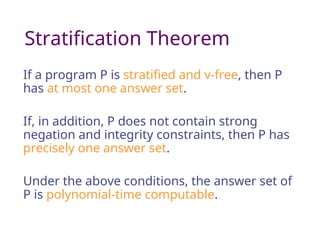
Stratification Theorem
If a program P is stratified and v-free, then P
has at most one answer set.
If, in addition, P does not contain strong
negation and integrity constraints, then P has
precisely one answer set.
Under the above conditions, the answer set of
P is polynomial-time computable.

Head-Cycle Free Programs
Idea: Forbid recursion through disjunction.
P is head-cycle free if there is a level mapping
|| ||h of P such that for every rule r of P:
 For any atom l in Body+(r), and for any l' in Head(r),
|| l ||h <= || l’ ||h ;
 For any pair of atoms, l and l’ in Head(r),
|| l ||h <> || l’ ||h

Head-Cycle Free Programs -
Example
P3: a v b.
a :- b.
P3 is head-cycle free:
|| a ||h = 2; || b ||h = 1

Head-Cycle Free Programs -
Example
P4: a v b.
a :- b.
b :- a.
P4 is not head-cycle free:
No head-cycle free level mapping exists;
there is recursion through disjunction!

Head-Cycle Free Theorem
Every head-cycle free program P is equivalent
to an v-free program shift(P) where disjunction
is “shifted” to the body.
P: a v b :- c. shift(P): a :- c, not b.
b :- c, not
a.

Complexity of Answer Set
Checking
{} nots not
{} P P P
vh P P P
v coNP coNP coNP

Complexity of Brave Reasoning
{} nots w w,nots not w, not
{} P P P P NP P
2
vh NP NP P
2 P
2 NP P
2
V P
2 P
2 P
3 P
3 P
2 P
3
Completeness under Logspace reductions

Intuitive Explaination
Three main sources of complexity:
1. exponential number of answer set
“candidates”;
2. difficulty of checking whether a candidate M is
an answer set of Rules(P) (Minimality of M can
be disproved by exponentially many subsets);
3. difficulty of determining optimality of the
answer set wrt. weak constraints.
Absence of source 1 eliminates both sources 2 and 3!

Complexity of Cautious Reasoning
{} nots w w,nots not w, not
{} P P P P
coN
P
P
2
Vh coNP coNP P
2 P
2
coN
P
P
2
V coNP P
2 P
3 P
3 P
2 P
3
Note that < V, {} > is “only” coNP-complete!

Bibliography: Foundations of DLP/ASP
 M. Gelfond and V. Lifschitz, Classical Negation in Logic
Programs and Disjunctive Databases. New Generation
Computing, 9:365-385, 1991.
 J. Minker. On Indefinite Data Bases and the Closed World
Assumption. In Proceedings 6th Conference on
Automated Deduction (CADE '82), D. Loveland, Ed.
Number 138 in Lecture Notes in Computer Science.
Springer, New York, 1982, pp. 292--308.
 N. Leone, P. Rullo, F. Scarcello, Disjunctive Stable Models:
Unfounded Sets, Fixpoint Semantics and Computation,
Information and Computation, Academic Press, New
York, Vol. 135, N. 2, 15 June 1997, pp. 69-112.

Bibliography: Knowledge
Representation
 M. Gelfond, N. Leone, Logic Programming and
Knowledge Representation --- the A-Prolog perspective.
Artificial Intelligence, Elsevier, 138(1&2), June, 2002.
 F. Buccafurri, N. Leone, P. Rullo, Enhancing Disjunctive
Datalog by Constraints. IEEE Transactions on Knowledge
and Data Engineering, 12(5) 2000, pp 845-860.
 T. Eiter, W. Faber, N. Leone, G. Pfeifer. Declarative
Problem-Solving Using the DLV System. In Jack Minker,
editor, Logic-Based Artificial Intelligence, pages 79-103.
Kluwer Academic Publishers, 2000.

Bibliography: DLV System (Overview)
 T. Eiter, N. Leone, C. Mateis, G. Pfeifer, F. Scarcello, The
Knowledge Representation System dlv: Progress Report,
Comparisons, and Benchmarks, in Proc. of KR'98, pp.
406-417, Morgan Kaufman, 1998.
 T. Eiter, W. Faber, N. Leone, G. Pfeifer, Declarative
Problem-Solving Using the DLV System in Logic in
Artificial Intelligence. J. Minker editor, Kluwer Academic
Publisher, 2000, pp 79-103.
 DLV Manual and Tutorial at http://www.dlvsystem.com

Bibliography: DLV (Algorithms and
Optimizations)
 W. Faber, N. Leone, G. Pfeifer, "Experimenting with Heuristics for
Answer Set Programming”. Proceedings of the 17th International
Joint Conference on Artificial Intelligence - IJCAI '01, Morgan
Kaufmann Publishers, Seattle, USA, August 2001, pp. 635-640.
 C. Koch, N. Leone, "Stable Model Checking Made Easy”.
Proceedings of the 16th International Joint Conference on
Artificial Intelligence - IJCAI '99, Morgan Kaufmann Publishers,
pp. 70-75, Stockolm, August 1999.
 N. Leone, S. Perri, F. Scarcello. “Improving ASP Instantiators by
Join-Ordering Methods”. Proceedings of the 6th International
Conference on Logic Programming and Non-Monotonic
Reasoning - LPNMR'01, LNAI 2173, Springer-Verlag, Vienna,
Austria, 17-19 September 2001.

jelia2002-tutorial.ppt answer set programming

More Related Content

Similar to jelia2002-tutorial.ppt answer set programming

More from kaliaragorn

Recently uploaded

jelia2002-tutorial.ppt answer set programming

Editor's Notes