Money: The Root of All Solutions
How Quantitative Easing Pull The Economy Out of the Great Recession
By Christopher Shanley
Introduction
One of the FED’s main purposes is to ensure the constant well being of
the economy. They accomplish this by maintaining the overnight interbank
lending rate, which is used to ensure that all banks have their required amount of
deposits on reserve at the end of the day. This overnight interbank lending rate is
known as the Federal Funds Rate. To ensure the economy stays in a constant
state the FED can manipulate this rate.1 They do this by increasing or decreasing
the amount of cash supply in the economy by means of purchasing or selling
securities, usually low risk short term treasury bonds.
In economic crisis banks supply of cash dwindles and the demand for
cash skyrockets, so the Federal Fund Rate increases because money is scarce.
The banks loose the ability to serve its customers needs because they need the
money to be kept on reserve and cannot lend it out to its customers. To solve this
problem the FED buys short-term low risk securities to increase the money
supply while lowering the demand for money. This will effectively lower the
Federal Funds Rate and the economy should recover. But what if it doesn’t?
Throughout the past seven years the Federal Reserve (FED) has initiated
a program of quantitative easing (QE) which directly infuses money into certain
1 This serves as bases of economic regulation in US economy and is not always
accurate.
areas of the economy. The goal of this process is to increase the supply of cash
in these struggling sectors of the economy to lower the long-term interest rate. In
doing this demand for investment in this sectors will increase, which will increase
the overall well being of the economy. This paper will be used to describe the
processes of the FEDs recent QE programs in comparison to other similar
programs used globally. Then it will discuss the impact of the programs on the
present economy’s health and discuss speculations of the future impacts of the
economy in relations to these programs.
When the FED lowered the Federal Funds Rates from 5% to nearly 0% in
2008 the crisis in theory should have been solved, but it didn’t. The factors that
caused this crisis we based on the creation of mortgaged backed securities and
subprime mortgage loan defaults. The creation of mortgaged backed securities
(MBS) fed the demand for more mortgages, which in turn relaxed regulations on
subprime lending. Subprime borrowers were now able to get mortgages on loans
that under previous circumstances they could not. In 2006 the housing credit
bubble burst when many of these subprime borrower could not make the
payments and defaulted on their loans. This cause the eventual collapse of MBS
market threw the US economy like many others into turmoil. As stated before the
FED lowered the Federal Funds Rate to an all time low and there was no
improvement. Many central banks around the world had to turn to unconventional
means to stimulate the economy.
Unconventional Stimuli: Quantitative Easing
In this section we will discuss the different forms of quantitative easing
(QE) used in the US by the FED and other centralized banks around the world.
QE is the process of buying unconventional securities for two reasons. (1)
To supply more money into the economy, (2) to liquated certain struggling
markets. In late 2008 and early 2009 that is exactly what the FED did. They
increased the money supply of the US economy by 1.775 trillion purchasing
assets like MBS, government sponsored enterprise debt and long-term treasury
bonds. Similar, the Bank of England in the same period of time launch an asset
purchasing program of their own to help stabilizes their economy. While
European Central Bank and Bank of Japan had QE programs in place at the
same time, their programs focused around directly lending money to banks.
The first QE program used by the FED uniquely isolated certain struggling
areas of the economy (e.g. mortgaged backed securities market, government
sponsored enterprise, as well as banks). Krishnamurthy and Vissing-Jorgensen
(2011) state, “For riskier bonds such as lower grade corporate bonds and MBS,
QE1 had affects through a reduction in default risk/default risk premia and a
reduced prepayment risk premium”. It also lowered yields on low risk long-term
bonds. The FED purchased these bonds by issuing reserve, increasing the
monetary base by 29%2. One of the major accomplishments of this the first QE
program was on the receiving side of the stimulus. Banks voluntary held the
excess supply cash in reserve deposits instead of using it to lend out to
2 This information was created by myself using data from Federal Reserve
customers. This provided the economy with the necessary time to react properly
to the stimulus.
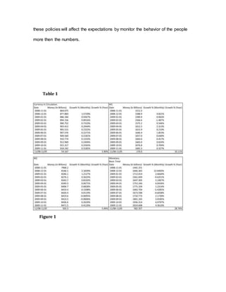
In the process of the first QE program we can notice many economic
factors. First the quantity equation from the quantity theory of money was not
effect. While the monetary base did rise 29%, mostly all other money supply
factors stayed relative to constant growth. The reasons I concluded was by
looking at the M1, M2, and currency in circulation growth from November 1, 2008
to November 1, 2009 in comparison to monetary base growth for the same
period. The only inference I could conclude was that while the supply of money
had risen banks did not use the excess supply, this kept M2 relatively growth
normal. My findings can be found in Table 1.
The second QE came in late 2010 with a new purpose behind it. Unlike
the first QE program the second program was designed to increase the still
stagnate economy. This program, usually called “QE2,” was explicitly designed to
lower long-term real interest rates and increase the inflation rate to levels
deemed more consistent with the Fed’s mandate from Congress (Fawley and
Neely 2013). Understanding rational expectations, when the FED announced the
second QE program would take affect in the future, inflation and bond yields
already adapted to the new monetary policy. This meant the overall effectiveness
of the program was not as efficient as the first program when it came yield shift
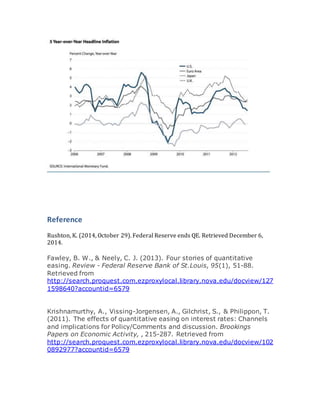
but as Figure 1 shows inflation rose nearly two percent in the first half of 2011.
Inflation was the key importance in this second QE program; Chairman Bernanke
understood that in fundamental economics constant inflation growth translates to
growth of GDP.
The importance of this program is shown by later data because this
program was put in place to satisfy short-term needs in the economy. As
described by the effects of the Phillips Curve, once people adapt and adjust to
their expectations of inflation, unemployment will adjust to the natural rate it was
and inflation will readjust to the unemployment rate. This caused expectations of
another recession in the late summer of 2011. The FED reacted to these spikes
by setting up a new program to inverse the long-term bond rates relative to the
short-term rates. The program was nicknamed “Operation Twist” because the
Fed sold $400 billion in short-term assets while purchasing $400 billion in long-
term assets (Fawley and Neely 2013).
Along with “Operation Twist” the FED implemented the now final program
of QE that was created to purchase $40 billion in MBS and $45 billion in long-
term treasuries a month. This program finished last month. The effects of this last
program have not seen substantially impact on the economy at this point.
Aftermath of Quantitative Easing
In review of the last section the Fed and similar central banks from the
largest economies all went into a major recession in 2008. At the end of 2014 we
can see that most of these economies in the short run have recovered. The US
monetary base increase by more the four times the size, unemployment is at
5.8%, and inflation is at 1.66%. Understanding these factors, this section will
provide speculative forecasting for short run and long run effects the quantitative
easing programs will have on the future economy using my understanding
economic principle and theories.
First, from understanding the IS function on the IS-LM curve we should
expect GDP to rise in the next year. This is because the real interest rates are
expected to relatively low. When interest rates remain low, planned expenditures
will rise, which in total raises GDP. Katherine Rushton (2014) reported,
“businesses are making more “fixed” investments in things like acquisitions and
buildings.” Statements like this show that the programs in the short run have
major benefits to short-term growth.
On the LM side of the curve we have the effects of money supply on GDP.
The FED throughout the past 7 years has injected the economy with huge stimuli
that have helped the economy sustain growth. In understanding the LM curve we
can see that the rise in money stock over the CPI makes the interest rates fall
and increase in output. This brings us to an interesting point; the FED continually
shocked the system with an influx of money, this created the environment where
interest rates fall, planned expenditures increase, and overall GDP rises. This all
seems like positive growth but as expectations adjusts in the future without QE
will everything remain constant or will be similar to the recession the US
economy was just in.
This is an excerpt from The Telegraph on recent activity in the stock
market since the end of the QE programs.
However, US markets remain vulnerable. Earlier this month, the S&P 500
erased its gains for the year amid fears over weakening economic growth in
Europe and Asia. The Dow Jones Industrial Average came close to doing the
same, as it dropped more than 400 points, or 3pc, in a single day. (Rushton,
2014)
The article goes on to state that the recovery of the market was because of the
FED hinting towards a fourth program. This shows that the economy has
adjusted to expect the Federal Reserve to use its resources to keep the economy
out of a recession.
My speculative long term forecast for the economy post QE programs is that
the economy needs time to adjust. The expectations of the effects on the
previous programs have not been in place for the proper length of time to make
accurate forecasting predictions. Quantitative Easing is very difficult to
comprehend, the policymakers that put these plan into affect still don’t fully
understand the complexity of the programs. As we grow with the decision we
made we will learn the benefits and costs of the programs in the future. Then we
can make more accurate decisions.
As the Lucas Critique states “it is naive to try to predict the effects of a
change in economic policy entirely on the basis of relationships observed in
historical data, especially highly aggregated historical data.” We can use this
information we receive from the effects of QE as base point in understanding
how to solve the next crisis or recession. To simply copy the same program in
the future will not guarantee the same success. What need to be learned is how
these policies will affect the expectations by monitor the behavior of the people
more then the numbers.
Figure 1
Table 1
Reference
Rushton, K. (2014, October 29). Federal Reserve ends QE. Retrieved December 6,
2014.
Fawley, B. W., & Neely, C. J. (2013). Four stories of quantitative
easing. Review - Federal Reserve Bank of St.Louis, 95(1), 51-88.
Retrieved from
http://search.proquest.com.ezproxylocal.library.nova.edu/docview/127
1598640?accountid=6579
Krishnamurthy, A., Vissing-Jorgensen, A., Gilchrist, S., & Philippon, T.
(2011). The effects of quantitative easing on interest rates: Channels
and implications for Policy/Comments and discussion. Brookings
Papers on Economic Activity, , 215-287. Retrieved from
http://search.proquest.com.ezproxylocal.library.nova.edu/docview/102
0892977?accountid=6579

Econ Term Paper

  • 1.
    Money: The Rootof All Solutions How Quantitative Easing Pull The Economy Out of the Great Recession By Christopher Shanley Introduction One of the FED’s main purposes is to ensure the constant well being of the economy. They accomplish this by maintaining the overnight interbank lending rate, which is used to ensure that all banks have their required amount of deposits on reserve at the end of the day. This overnight interbank lending rate is known as the Federal Funds Rate. To ensure the economy stays in a constant state the FED can manipulate this rate.1 They do this by increasing or decreasing the amount of cash supply in the economy by means of purchasing or selling securities, usually low risk short term treasury bonds. In economic crisis banks supply of cash dwindles and the demand for cash skyrockets, so the Federal Fund Rate increases because money is scarce. The banks loose the ability to serve its customers needs because they need the money to be kept on reserve and cannot lend it out to its customers. To solve this problem the FED buys short-term low risk securities to increase the money supply while lowering the demand for money. This will effectively lower the Federal Funds Rate and the economy should recover. But what if it doesn’t? Throughout the past seven years the Federal Reserve (FED) has initiated a program of quantitative easing (QE) which directly infuses money into certain 1 This serves as bases of economic regulation in US economy and is not always accurate.
  • 2.
    areas of theeconomy. The goal of this process is to increase the supply of cash in these struggling sectors of the economy to lower the long-term interest rate. In doing this demand for investment in this sectors will increase, which will increase the overall well being of the economy. This paper will be used to describe the processes of the FEDs recent QE programs in comparison to other similar programs used globally. Then it will discuss the impact of the programs on the present economy’s health and discuss speculations of the future impacts of the economy in relations to these programs. When the FED lowered the Federal Funds Rates from 5% to nearly 0% in 2008 the crisis in theory should have been solved, but it didn’t. The factors that caused this crisis we based on the creation of mortgaged backed securities and subprime mortgage loan defaults. The creation of mortgaged backed securities (MBS) fed the demand for more mortgages, which in turn relaxed regulations on subprime lending. Subprime borrowers were now able to get mortgages on loans that under previous circumstances they could not. In 2006 the housing credit bubble burst when many of these subprime borrower could not make the payments and defaulted on their loans. This cause the eventual collapse of MBS market threw the US economy like many others into turmoil. As stated before the FED lowered the Federal Funds Rate to an all time low and there was no improvement. Many central banks around the world had to turn to unconventional means to stimulate the economy.
  • 3.
    Unconventional Stimuli: QuantitativeEasing In this section we will discuss the different forms of quantitative easing (QE) used in the US by the FED and other centralized banks around the world. QE is the process of buying unconventional securities for two reasons. (1) To supply more money into the economy, (2) to liquated certain struggling markets. In late 2008 and early 2009 that is exactly what the FED did. They increased the money supply of the US economy by 1.775 trillion purchasing assets like MBS, government sponsored enterprise debt and long-term treasury bonds. Similar, the Bank of England in the same period of time launch an asset purchasing program of their own to help stabilizes their economy. While European Central Bank and Bank of Japan had QE programs in place at the same time, their programs focused around directly lending money to banks. The first QE program used by the FED uniquely isolated certain struggling areas of the economy (e.g. mortgaged backed securities market, government sponsored enterprise, as well as banks). Krishnamurthy and Vissing-Jorgensen (2011) state, “For riskier bonds such as lower grade corporate bonds and MBS, QE1 had affects through a reduction in default risk/default risk premia and a reduced prepayment risk premium”. It also lowered yields on low risk long-term bonds. The FED purchased these bonds by issuing reserve, increasing the monetary base by 29%2. One of the major accomplishments of this the first QE program was on the receiving side of the stimulus. Banks voluntary held the excess supply cash in reserve deposits instead of using it to lend out to 2 This information was created by myself using data from Federal Reserve
  • 4.
    customers. This providedthe economy with the necessary time to react properly to the stimulus. In the process of the first QE program we can notice many economic factors. First the quantity equation from the quantity theory of money was not effect. While the monetary base did rise 29%, mostly all other money supply factors stayed relative to constant growth. The reasons I concluded was by looking at the M1, M2, and currency in circulation growth from November 1, 2008 to November 1, 2009 in comparison to monetary base growth for the same period. The only inference I could conclude was that while the supply of money had risen banks did not use the excess supply, this kept M2 relatively growth normal. My findings can be found in Table 1. The second QE came in late 2010 with a new purpose behind it. Unlike the first QE program the second program was designed to increase the still stagnate economy. This program, usually called “QE2,” was explicitly designed to lower long-term real interest rates and increase the inflation rate to levels deemed more consistent with the Fed’s mandate from Congress (Fawley and Neely 2013). Understanding rational expectations, when the FED announced the second QE program would take affect in the future, inflation and bond yields already adapted to the new monetary policy. This meant the overall effectiveness of the program was not as efficient as the first program when it came yield shift but as Figure 1 shows inflation rose nearly two percent in the first half of 2011. Inflation was the key importance in this second QE program; Chairman Bernanke
  • 5.
    understood that infundamental economics constant inflation growth translates to growth of GDP. The importance of this program is shown by later data because this program was put in place to satisfy short-term needs in the economy. As described by the effects of the Phillips Curve, once people adapt and adjust to their expectations of inflation, unemployment will adjust to the natural rate it was and inflation will readjust to the unemployment rate. This caused expectations of another recession in the late summer of 2011. The FED reacted to these spikes by setting up a new program to inverse the long-term bond rates relative to the short-term rates. The program was nicknamed “Operation Twist” because the Fed sold $400 billion in short-term assets while purchasing $400 billion in long- term assets (Fawley and Neely 2013). Along with “Operation Twist” the FED implemented the now final program of QE that was created to purchase $40 billion in MBS and $45 billion in long- term treasuries a month. This program finished last month. The effects of this last program have not seen substantially impact on the economy at this point. Aftermath of Quantitative Easing In review of the last section the Fed and similar central banks from the largest economies all went into a major recession in 2008. At the end of 2014 we can see that most of these economies in the short run have recovered. The US monetary base increase by more the four times the size, unemployment is at 5.8%, and inflation is at 1.66%. Understanding these factors, this section will
  • 6.
    provide speculative forecastingfor short run and long run effects the quantitative easing programs will have on the future economy using my understanding economic principle and theories. First, from understanding the IS function on the IS-LM curve we should expect GDP to rise in the next year. This is because the real interest rates are expected to relatively low. When interest rates remain low, planned expenditures will rise, which in total raises GDP. Katherine Rushton (2014) reported, “businesses are making more “fixed” investments in things like acquisitions and buildings.” Statements like this show that the programs in the short run have major benefits to short-term growth. On the LM side of the curve we have the effects of money supply on GDP. The FED throughout the past 7 years has injected the economy with huge stimuli that have helped the economy sustain growth. In understanding the LM curve we can see that the rise in money stock over the CPI makes the interest rates fall and increase in output. This brings us to an interesting point; the FED continually shocked the system with an influx of money, this created the environment where interest rates fall, planned expenditures increase, and overall GDP rises. This all seems like positive growth but as expectations adjusts in the future without QE will everything remain constant or will be similar to the recession the US economy was just in. This is an excerpt from The Telegraph on recent activity in the stock market since the end of the QE programs.
  • 7.
    However, US marketsremain vulnerable. Earlier this month, the S&P 500 erased its gains for the year amid fears over weakening economic growth in Europe and Asia. The Dow Jones Industrial Average came close to doing the same, as it dropped more than 400 points, or 3pc, in a single day. (Rushton, 2014) The article goes on to state that the recovery of the market was because of the FED hinting towards a fourth program. This shows that the economy has adjusted to expect the Federal Reserve to use its resources to keep the economy out of a recession. My speculative long term forecast for the economy post QE programs is that the economy needs time to adjust. The expectations of the effects on the previous programs have not been in place for the proper length of time to make accurate forecasting predictions. Quantitative Easing is very difficult to comprehend, the policymakers that put these plan into affect still don’t fully understand the complexity of the programs. As we grow with the decision we made we will learn the benefits and costs of the programs in the future. Then we can make more accurate decisions. As the Lucas Critique states “it is naive to try to predict the effects of a change in economic policy entirely on the basis of relationships observed in historical data, especially highly aggregated historical data.” We can use this information we receive from the effects of QE as base point in understanding how to solve the next crisis or recession. To simply copy the same program in the future will not guarantee the same success. What need to be learned is how
  • 8.
    these policies willaffect the expectations by monitor the behavior of the people more then the numbers. Figure 1 Table 1
  • 9.
    Reference Rushton, K. (2014,October 29). Federal Reserve ends QE. Retrieved December 6, 2014. Fawley, B. W., & Neely, C. J. (2013). Four stories of quantitative easing. Review - Federal Reserve Bank of St.Louis, 95(1), 51-88. Retrieved from http://search.proquest.com.ezproxylocal.library.nova.edu/docview/127 1598640?accountid=6579 Krishnamurthy, A., Vissing-Jorgensen, A., Gilchrist, S., & Philippon, T. (2011). The effects of quantitative easing on interest rates: Channels and implications for Policy/Comments and discussion. Brookings Papers on Economic Activity, , 215-287. Retrieved from http://search.proquest.com.ezproxylocal.library.nova.edu/docview/102 0892977?accountid=6579