The thesis explores the integration of BCH-LDPC concatenated coding with high-order modulation schemes for satellite transmitters, emphasizing the importance of choosing effective modulation and coding schemes to achieve reliable data transmission. It details the development of versatile coding techniques like bit-interleaved coded modulation (BICM) and advanced forward error correction methods, particularly within the context of the DVB-S2 standard and its application in adaptive coding modulation systems. The work concludes with hardware implementation insights and preliminary testing results demonstrating the efficiency and performance capabilities of the designed system.

1. POLITECNICO DI TORINO
III Facoltà diIngegneria
Corso di Laurea in Ingegneria delle Telecomunicazioni
Tesi di Laurea Magistrale
BCH-LDPC Concatenated Coding
and High Order Modulations for
Satellite Transmitters
Relatore:
prof. Roberto Garello
Candidato:
Eriprando Pacces
Supervisore aziendale
Thales Alenia Space Italia
ing. Domenico Giancristofaro
Luglio 2008

2. II

3. Summary
In every communication system, choice and project of modulation schemes are both
aimed at transmitting data reliably enough for the type of operating scenario, while
making an efficient use of the available resources (e.g., bandwidth, power, weight
and encumbrance of equipment)
In 1948, Claude E. Shannon defines and quantifies information. Furthermore,
he is able to demonstrate that, for any given transmission rate being less or equal
to channel capacity, there exists a coding scheme capable of attaining an error
probability arbitrarily small, thus having a completely reliable communication.
Unfortunately, Shannon’s theorem does not give any indication on how to find
out these coding schemes. Shannon proves, however, that long randomly chosen
codes provide a low average error probability. Unfortunately, a direct realization of
those codes mentioned above has a quite unattractive complexity.
From 1948, therefore, the most of engineers’ effort starts focusing on the develop-
ment of coding and modulation scheme capable of getting closer to Shannon limit.
In spite of the initial pessimism (let us think about the “good codes are messy” motto
which goes around among code scientists), the problem gets solved at least for the
best case scenario, that is, over AWGN channel.
In 80s, then, the better understanding of the meaning of Shannon’s Theorem
leads to a revision of the paradigm used as far on the field of modulation and coding.
These two disciplines, which earlier are developing independently, start to become
more entangled.
The need of attaining high spectral efficiencies pulls up the modulation dimension
(i.e., the number of waveforms per symbol). Meanwhile, even more powerful error cor-
recting codes are conceived. In such context, Ungerboek’s work fosters TCM (Trellis
Coded Modulation) advent, making clear the advantages of treating modulation and
coding as a single unit.
Moreover, various schemes published in literature prove that the jointly use
of turbo codes (a coding technique introduced by Claude Berrou) and TCM can
be profitable. However, turbo codes should be designed ad hoc for every single
modulation, an unpractical solution for systems using a few constellation. The
solution of this problem is called Bit Interleaved Coding Modulation (BICM), thanks
III

4. to which it is possible to obtain outstanding results employing an only one solution
for all the expected modulations.This big flexibility makes BICM commercially very
attractive for broadband ACM (Adaptive Coding Modulation) based communications
which require a wide range of spectral spectral efficiencies. DVB-S2 as well as the
novel MOHMS (which is about to be standardized by CCSDS) solution exploit ACM
techniques.
The DVB-S2 standard employs most of the cutting-edge techniques within the
coding and (high order) modulation field. The coding ’engine’ (i.e., the essential
element) is composed by an LDPC concatenated to a BCH in order to limit the
typical drop of performance at higher signal to noise ratio, namely, the error floor.
This standard should insure performance between 0,6dB and 1,2dB from Shannon’s
limit. In addition to this, DVB-S2, offering a great amount of operating modes, is
suitable for many kinds of spatial mission. The high regularity and periodicity of
the LDPC structure, then, guarantees a reasonable complexity at the receiver.
Let us now start to summarize the thesis contents.
After a brief introduction devoted to outline the principal characteristics and
applications of satellite communications (e.g. broadcasting TV services, remote
sensing, data gathering, etc.), we will describe the functional blocks of DVB-S2
Tx Section. We will put in evidence how the ACM technique could guarantee a
higher throughput, a greater service availability (especially if compared with that we
would get by using a plain CCM), a greater efficiency and optimization of spacecraft
resources. Then we will go on overhauling DVB-S2 FEC (Forward Error Correction).
After a brief description of the main methods used to build up BCH codes, we will
illustrate the principal characteristic of the particular BCH employed by DVB-S2,
diving then into LDPC description. Once in there, we will try to give a justification
over their renaissance along with explaining their structure, methods, and coding
algorithms with a special focus on their iterative message passing decoding.
The central part of thesis is devoted to analysis and study of fast BCH coding
algorithms together with their HW realization.
After a preliminary phase of analysis on the traditional BCH encoding algorithm,
we will describe a set of architecture capable of implementing the encoding, while
analyzing cons and pros from the HW perspective. These simple architectures are
intrinsically serial and, therefore, slow; they are called Linear Feedback Shift Register
(LSFR) and they implement the division by polynomial code generator. Cyclic codes,
whose family BCH codes belong, are typically encoded in that manner.
From a HW point of view, the DVB-S2 codeword length, the frequency constraints,
and the parallel interface of LDPC encoder will require the development of a parallel
BCH encoder in order to meet the speed and integration requirements.
The mathematical description of the parallel algorithm and, in particular, the
fortunate properties of the state matrix boiled down from the system will lead to a
very efficient implementation of the BCH encoder.
IV

5. The choice of the HW architecture and its degree of parallelism will be dictated,
as mentioned earlier, not only by constraints imposed for the realized transmission
section, but especially by the requirement of making the encoder work in ACM.
According to ETSI, in fact, either modulation or coding can vary on a frame basis.
This feature implies the storage into LUT all the matrices coefficients associated to
each correcting capability of BCH code. The HW architecture includes a 192 bit
register, two blocks of 192 combinatorial network whose behavioral is programmed
by coefficients stored in LUTs, and a few sum blocks, that is, XOR gates. These
combinatorial networks are actually 8 bit XOR gates whose inputs are enabled by
bits stored into dedicated LUTs. This makes possible the encoding of DVB-S2 for
each operating mode without modifying the general encoder architecture. More in
depth, the all boils down to inhibit either 32 or 64 couples of combinatorial networks
depending on the BCH error correcting capability.
In another chapter we will present simulation of algorithms and architectures
set up in C/C++ in order to give support and a data reference to VLSI (Very
Large Scale Integration) designers for the architecture description and the synthesis
validation. All of that, though, not before having verified by means of an adequate
number of simulation in C/C++ that the generated codewords succeeding in doing
their job, that is, correcting at least the expected number of errors they are supposed
to correct. To check that, we will use the Berlekamp-Massey algorithm which, by
the way, enable to avoid a costly matrix inversion since it exploits the linear (LFSR)
relation between code syndrome and polynomial coefficients, thus making possible
to find out error locations where error occurred during transmission. Needless to
say, for that reason, this polynomial is called error locator. To perform decoding or
only error detection, we need to know the Galois Field where polynomial generator’s
roots lay and therefore study thoroughly the DVB-S2 BCH structure so that being
capable of building up handy tables to perform operations required at decoder side.
At the end, the last part of thesis will even show results achieved as far, gathered
throughout the testing phases performed over the entire DVB-S2 TX section set up
in laboratory. At the time we are writing, the functional verification is still running
onto a prototyping FPGA, Altera EP180 Stratix II, board. Unfortunately, the BER
end-to-end test is still missing, but the performance of high order modulation section
has been just evaluated.
In the last description we briefly illustrate the architecture and blocks of the entire
section, we show results, obtained by interconnecting a broadband VSA (Vector Signal
Analyzer) demodulating the received signal to an Agilent digital oscilloscope, in
terms of two statistical measure over the constellations: the phase and the amplitude
error. Last but not less important, we tackle a problem coming out at the higher
symbol rate, that is, the amplitude distortion at the DAC output. Our measures
clearly shows importance of pre-compensation filters when the transmission rate
become higher.
V

6. Acknowledgements
I thank the Prof.dr. Roberto Garello which has given me the opportunity, introduc-
ing to the Eng.dr. Domenico Giancrostofaro, of working into the Algorithms and
Architectures Division of Thales Alenia Space.
I would like to thank the Thales Alenia Space in L’Aquila and, particularly, the
above mentioned division for having put at my disposal all the necessary tools and
piece of equipment in order to accomplish my goals.
I am grateful to Domenico Giancristofaro who, in spite of his numerous duties,
followed and supported me constantly and patiently throughout the development of
my activity in TAS-I.
Finally, a last thank to Cinzia Moca and Massimo Fonte, which provided me
excellent insights and advices while I was writing and performing the work presented
here.
VI

7. Contents
Summary III
Acknowledgements VI
1 Applications and Features of Satellite Communications 1
1.1 Introduction . . . . . . . . . . . . . . . . . . . . . . . . . . . . . . . . 1
1.2 Remote Sensing and Earth Observation . . . . . . . . . . . . . . . . . 3
1.3 The Second Generation of Digital Video Broadcasting System . . . . 6
2 DVB-S2 MODEM Concepts and Architecture 9
2.1 Modulation and Coding Schemes . . . . . . . . . . . . . . . . . . . . 9
2.1.1 BICM: How to Obtain Top Performance Using a Single Code
and Various Modulations . . . . . . . . . . . . . . . . . . . . . 10
2.1.2 Choice of Modulation Scheme . . . . . . . . . . . . . . . . . . 10
2.1.3 The Ultimate Bound to Compare Modem Performance . . . . 11
2.1.4 Adaptive Coding Modulation . . . . . . . . . . . . . . . . . . 15
2.2 ACM Modem System Description . . . . . . . . . . . . . . . . . . . . 17
2.2.1 Architecture and Sub-Blocks Specifications . . . . . . . . . . . 18
2.2.2 Sub-Blocks Description . . . . . . . . . . . . . . . . . . . . . . 19
2.3 Inner and Outer FEC . . . . . . . . . . . . . . . . . . . . . . . . . . . 25
2.3.1 BCH . . . . . . . . . . . . . . . . . . . . . . . . . . . . . . . . 26
2.3.2 LDPC . . . . . . . . . . . . . . . . . . . . . . . . . . . . . . . 29
2.4 Modem Performance . . . . . . . . . . . . . . . . . . . . . . . . . . . 38
3 BCH Encoding Algorithms for DVB-S2 Digital Transmissions 43
3.1 Encoding Algorithm Description . . . . . . . . . . . . . . . . . . . . . 43
3.2 Serial Architectures . . . . . . . . . . . . . . . . . . . . . . . . . . . . 46
3.3 Encoding Algorithms for Parallel Architectures . . . . . . . . . . . . 47
3.3.1 Modelling System . . . . . . . . . . . . . . . . . . . . . . . . . 47
3.3.2 Parallel Linear System Description . . . . . . . . . . . . . . . 49
3.3.3 Matrices Structure and Properties . . . . . . . . . . . . . . . . 50
VII

8. 3.4 Some Considerations . . . . . . . . . . . . . . . . . . . . . . . . . . . 52
4 Hardware Implementation of BCH Encoder 53
4.1 FEC Encoding Section . . . . . . . . . . . . . . . . . . . . . . . . . . 53
4.2 Encoder Description . . . . . . . . . . . . . . . . . . . . . . . . . . . 55
4.3 Dealing with Each Error Protection . . . . . . . . . . . . . . . . . . . 56
4.4 Interface and Parity Bits Extraction . . . . . . . . . . . . . . . . . . . 58
4.5 Frequency and Memory Requirements . . . . . . . . . . . . . . . . . . 59
5 Software Package for VHDL Validation 65
5.1 Software Implementation of Serial Encoder . . . . . . . . . . . . . . . 65
5.2 Software Implementations of Parallel Encoder . . . . . . . . . . . . . 66
5.3 Galois Fields Tables . . . . . . . . . . . . . . . . . . . . . . . . . . . . 70
5.4 Decoding BCH . . . . . . . . . . . . . . . . . . . . . . . . . . . . . . 71
5.4.1 Error Detection . . . . . . . . . . . . . . . . . . . . . . . . . . 71
5.4.2 Berlekamp-Massey Algorithm . . . . . . . . . . . . . . . . . . 72
5.4.3 Chien Search . . . . . . . . . . . . . . . . . . . . . . . . . . . 77
5.5 Software Robustness and Validation . . . . . . . . . . . . . . . . . . . 77
5.5.1 Error Pattern Generation . . . . . . . . . . . . . . . . . . . . 78
5.5.2 The C Code . . . . . . . . . . . . . . . . . . . . . . . . . . . . 78
6 Preliminary Laboratory Test of DVB-S2 TX Section 89
6.1 Introduction . . . . . . . . . . . . . . . . . . . . . . . . . . . . . . . . 89
6.2 Test Objectives and Setup . . . . . . . . . . . . . . . . . . . . . . . . 93
6.3 Test Results . . . . . . . . . . . . . . . . . . . . . . . . . . . . . . . . 96
6.3.1 2 MBaud — 16 APSK . . . . . . . . . . . . . . . . . . . . . . 96
6.3.2 30 MBaud — 8 PSK . . . . . . . . . . . . . . . . . . . . . . . 98
6.3.3 30 MBaud — 16 APSK . . . . . . . . . . . . . . . . . . . . . . 100
6.4 64-APSK Modulator . . . . . . . . . . . . . . . . . . . . . . . . . . . 101
7 Conclusions 103
A Galois (or Finite) Fields 105
A.1 Algebraic Structures: a Glance . . . . . . . . . . . . . . . . . . . . . . 106
A.2 How Do We Get Galois Fields? . . . . . . . . . . . . . . . . . . . . . 107
A.3 A Mathematical Survey . . . . . . . . . . . . . . . . . . . . . . . . . 109
A.4 Irreducible and Primitive polynomials . . . . . . . . . . . . . . . . . . 110
A.5 Factoring xn − 1 . . . . . . . . . . . . . . . . . . . . . . . . . . . . . 111
VIII

9. B Cyclic Codes 115
B.1 Shift Operation . . . . . . . . . . . . . . . . . . . . . . . . . . . . . . 115
B.2 Rings of Polynomials and Ideals in Rings . . . . . . . . . . . . . . . . 116
B.3 Algebraic Description . . . . . . . . . . . . . . . . . . . . . . . . . . . 117
Bibliography 119
IX

10. Chapter 1
Applications and Features of Satellite
Communications
1.1 Introduction
Satellite communications provide unique solutions for a number of communications
and strategic applications that are possible only using the satellite environment.
These applications are typically niche applications, such as:
• Multimedia communications provided to wide geographical areas with low
population density; in this case the deployment of the satellite is less expensive
than the corresponding terrestrial network to provide the same service;
• Maritime communications (e.g. Inmarsat) also associated to radio-navigation
systems;
• Television broadcasting: in this case, a single signal is broadcasted for a wide
community of users, making more economically efficient the use of the satellite
when compared to a wide network of local broadcasting stations to cover the
geographical area;
• Earth observation and monitoring systems offering a distinctive potential for
strategic (military and commercial) information gathering.
All of the above applications require from medium to high data rate communica-
tion links, which need to be implemented with the resources typical of a spacecraft.
Clearly the onboard available power, weight and antenna size are limited: this leads
to the requirement of promoting state-of-the art research in the field of modulation
and coding, as well as synchronization techniques able to operate al close as possible
to the ultimate limits of performances, at very low signal to noise ratios and saving
1

11. 1 – Applications and Features of Satellite Communications
as much as possible the used bandwidth, which, besides, has to be shared among
various coexisting satellites as well as terrestrial applications.
Hence state-of-the-art satellite communications for Earth Observation and Tele-
communications (which are among the most appealing applications requiring high
data rate modems) are characterized by the need for both maximum information
throughput and minimum power and bandwidth consumption, requirements evidently
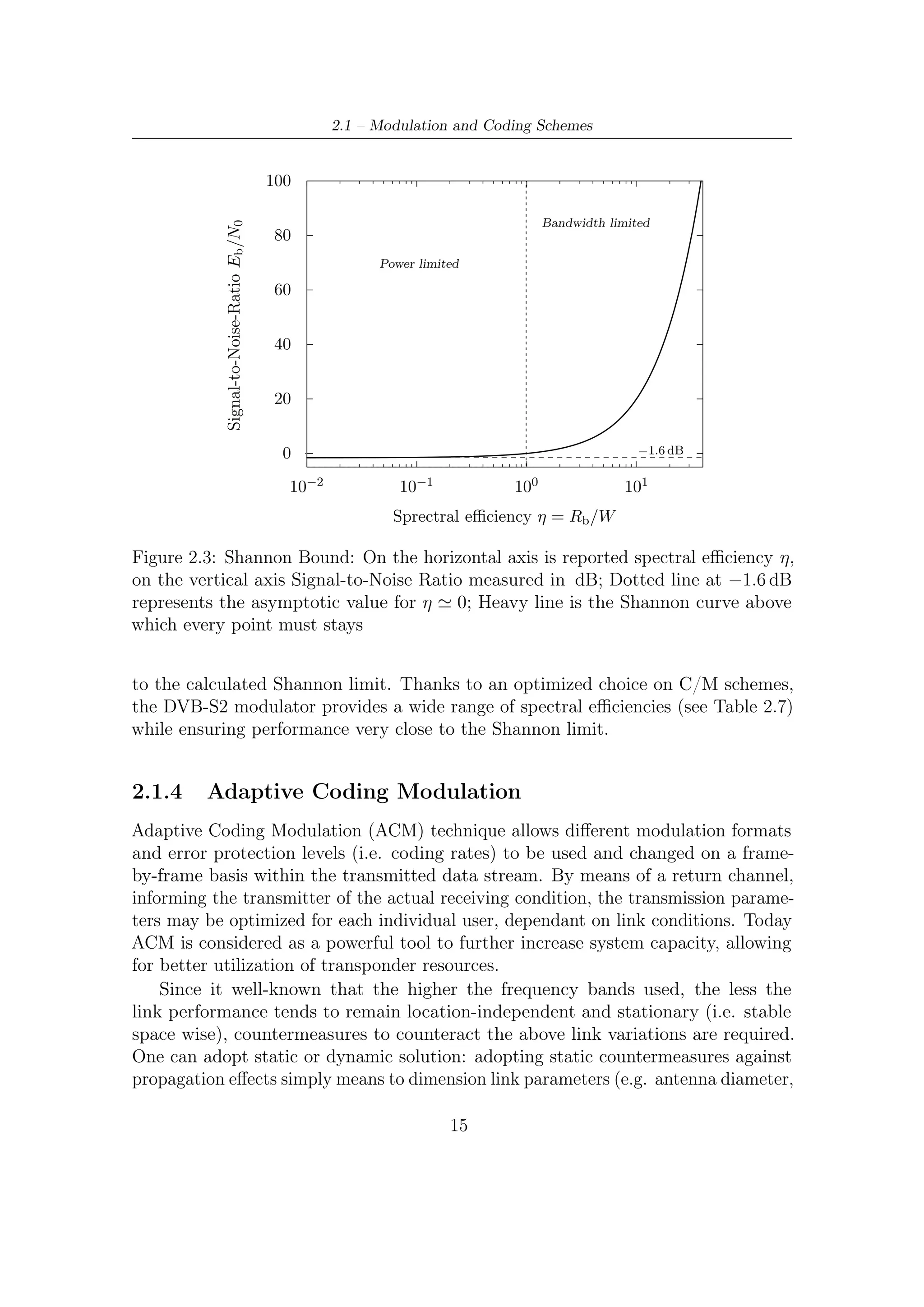
contradictory with an inter-relation theoretically stated by the Shannon Bound.
Additionally the available bandwidth, data rate and signal to noise ratio specifications
vary according to each specific mission/from one mission to another. An ideal all-
purpose MODEM unit, flexible for any mission application and hence commercially
appealing, should have the following features:
• Flexible configurability of data rate and bandwidth allocated;
• High variability of signal to noise ratio of operation;
• Performance always at 1 dB maximum from the Shannon Capacity Bound
(fixed modulation and coding quality);
• Efficient usage of power and hardware resources for processing.
Such a modem would allow having unique off-the-shelf solution, matching the needs
of almost all the missions for Earth Observation and extra-high-speed telecommuni-
cations.
The novel DVB-S2 modulation and coding scheme as well as the Modem for Higher
Order Modulation Schemes (MHOMS) performance are so close to the Shannon
Bound that they are expected to set the modulation and coding baseline for many
years to come. The MHOMS program was financed by European Space Agency
(ESA). The envisaged MHOMS modem application scenarios will encompass as a
minimum:
• High-speed distributed Internet access;
• Trunk connectivity (backbone/backhaul);
• Earth observation high-speed downlink;
• Point-to-multipoint applications (e.g., high-speed multicasting/broadcasting).
Further details on MHOMS are available in [19, 4].
2

12. 1.2 – Remote Sensing and Earth Observation
1.2 Remote Sensing and Earth Observation
Earth observation satellites have a key role to play in both the civilian and military
sectors, monitoring nearly all aspects of our planet. This is the only technology
capable of providing truly global coverage, particularly over the vast expanses of the
oceans and sparsely populated land areas (e.g. deserts, mountains, forests, and polar
regions). Earth observation data is being used by more than 300 research teams.
Small high-tech firms, large corporations and public agencies (meteorological offices,
etc.) use Earth-observation data for both operational and commercial purposes.
To provide professional services such as oceanography, meteorology, climatology,
etc. to the end user, Earth observation satellites requires a high capacity of acquiring
and processing a large volume of images on a daily basis. For example, COSMO-Sky-
Med, in full constellation configuration, can acquire up to 560 GB per day, roughly
corresponding to 1800 standard images.
COSMO-SkyMed interoperable system [20] is a remarkable example of a telecom-
munications integrated system capable of supporting the ability to exchange data
with other external observation systems according to agreed modalities and standard
protocols. The COSMO-SkyMed (Constellation of four Small Satellites for Mediter-
ranean basin Observation) is a low-orbit, dual-use Earth observation satellite system
operating in the X-band. It is funded by the Italian Ministry of Research (MIUR)
and Ministry of Defense and managed by the Italian space agency (ASI). COSMO-
SkyMed 1 has been successfully launched on June 7th, 2007 and COSMO-SkyMed 2
on December 10, 2007.
Thales Alenia Space is the program prime contractor, responsible for the devel-
opment and construction of the entire COSMO-SkyMed system, including the space
segment, with four satellites equipped with high resolution X-band synthetic aper-
ture radars (SAR) and the ground segment, a sophisticated turnkey geographically
distributed infrastructure. The ground segment is realized by Telespazio and in-
cludes the satellite control segment, mission planning segment, civilian user segment,
defense user segment, mobile processing stations and programming cells. Thales
Alenia Space is also responsible for the mission simulator, the integrated logistics
and all operations up to delivery of the constellation.
Three particular aspects characterize COSMO-SkyMed’s system performance:
the space constellation’s short revisit time for global Earth coverage; the short
system response time; and the multi-mode SAR instruments imaging performance.
COSMO-SkyMed features satellites using the most advanced remote sensing tech-
nology, with resolution of less than one meter, plus a complex and geographically
distributed ground segment produced by Italian industry. COSMO-SkyMed’s high
image performance relies on the versatile SAR instrument, which can acquire images
in different operative modes, and to generate image data with different (scene) size
and resolution (from medium to very high) so as to cover a large span of applicative
3

13. 1 – Applications and Features of Satellite Communications
needs.
Synthetic Aperture Radars (SARs) are most employed to gather a large amount
of high resolution images. In this field, Thales Alenia Space played an important
role in the development of the X-SAR (SAR operating in X band) space and ground
segments. X-SAR is a joint project between NASA, the German space agency
(DARA), and the Italian space agency (ASI) as part of NASA’s “Mission to Planet
Earth”. X-SAR can measure virtually any region of the Earth in all weather and
sunlight conditions, as well as penetrate vegetation, ice and dry sand, to map the
surface and provide scientists with detailed information on climatic and geological
processes, hydrological cycles and ocean circulation. X-SAR has flown on the U.S.
Space Shuttle twice, in April and September 1994, both times on Endeavour. The
two consecutive flights observed the same sites on Earth during two different seasons
in order to detect any seasonal changes, thus contributing to more precise and reliable
monitoring of renewable and nonrenewable resources. The SIR-C/X-SAR missions
observed more than 400 sites. Based on the knowledge acquired during these missions,
Thales Alenia Space participated in the Shuttle Radar Topography Mission (January
2000) which re-used the X-SAR radars to produce the first three-dimensional map of
the Earth’s surface.
Concerning the applications, the space constellations and versatility of the multi-
mode SAR instrument enable a wide variety of image data products with different
sizes, resolutions, elaboration levels, and accuracies (e.g. geo-localization), suit-
able for different applications needs, and allowing large environmental monitoring,
territory surveillance, intelligence applications, and critical phenomena detection.
By interferometric images, three-dimensional Digital Elevation Model products can
be obtained and used to render a city with buildings, streets, or high-resolution
topography.
COSMO-SkyMed mission specifications are compatible with numerous applica-
tions relating to civilian and military/security domains with 2D or 3D data. 2D
applications are mainly related to cartographic purpose. Other applications are
aimed at:
• Agricolture, for crop mapping and management;
• Landscape classification, for basic land use identification;
• Geology mapping for mineral, oil, and gas resources detection;
• Accurate urban area mapping for urban evolution surveys and management
(identification of high-density and low-density urban zones), as well as industrial
zone mapping with identification of buildings of interest, port implantations,
storage zones, airports, etc.;
4

14. 1.2 – Remote Sensing and Earth Observation
• Road and network (electricity, gas, telecom) identification and mapping, for
compiling the Geographic Information System (GIS) data base (note, e.g., its
relevance for applications such as radio navigation and safety of life services);
• Survey mapping.
Other applications fields concern hydrology, water resource inventory and detection,
coastal zones for erosion and coastal line determination. 3D possible applications are
various:
• Decision help: based on 3D models as powerful tools. They allow citizens, city
authorities and managements services to understand and explore a territory,
and to build up a database for realistic simulations. For example, architecture,
urbanization and new transport infrastructures can be simulated via a 3D
database and presented to the different city players;
• Natural and industrial risk management: simulation, prevention and post-crisis.
Using a Digital Elevation Model combined with a high-resolution image allows
phenomena simulation such as flood, fire, earthquake, air pollution, etc. It can
be used during different risk management phases, such as:
– Prevention: preparation of intervention missions, reports of risky areas to
survey, simulation of phenomena and related interventions;
– Crisis anticipation: types of risky building, communication network failure,
secondary itineraries to use, 3D localization of interesting positions (e.g.
helicopter landing zones);
– Post-crisis: damage evaluation, reconstruction planning.
In mid-2007 Italy and France have been activated a bilateral image-trading
protocol providing for reciprocal access to Helios 2 and COSMO-SkyMed data.
This agreement enabled the French and Italian armed forces to benefit from the
complementary optical and radar image capabilities of these systems.
This complex, challenging system delivers outstanding security, international
cooperation (for civilians and, within NATO countries, for defense), scalability
and interoperability. In other words, COSMO-SkyMed provides Italy and partner
countries with one of the worldŠs most technologically advanced observation systems
to guarantee greater security and an improved standard of living.
5

15. 1 – Applications and Features of Satellite Communications
1.3 The Second Generation of Digital Video Broad-
casting System
DVB-S2 is the second-generation DVB specification for broadband satellite applica-
tions, developed on the success of the first generation specifications (i.e. DVB-S for
broadcasting and DVB-DSNG for satellite news gathering and contribution services),
benefiting from the technological achievements of the last decade.
The DVB-S2 system has been designed for various broadband satellite applications
• broadcasting services of Standard Definition TeleVision (SDTV) and High
Definition TeleVision (HDTV);
• interactive applications oriented to professional or domestic services (i.e. Inter-
active Services including Internet Access for consumer applications);
• professional service of Satellite News Gathering (SNG);
• distribution of TV signals (VHF/UHF) to Earth digital transmitters;
• data distribution and Internet Trunking.
The DVB-S2 standard achieves a higher capacity of data transmission than the
first generation systems, an enhanced flexibility, a reasonable complexity 1 of the
receiver. In fact, it has been specified around three key concepts: best transmission
performance, total flexibility and reasonable receiver complexity.
To obtain a well balanced ratio between complexity and performance, DVB-
S2 benefits from more recent developments in channel coding and modulation.
Employment of these novel techniques translates in a 30 percent of capacity increase
over DVB-S under the same transmission conditions.
To achieve the top quality performance, DVB-S2 is based on LDPC (Low Density
Parity Check) codes, simple block codes with very limited algebraic structure,
discovered by R. Gallager in 1962. LDPC codes have an easily parallelizable decoding
algorithm which consists of simple operations such as addition, comparison and table
look-up; moreover the degree of parallelism is adjustable which makes it easy to
trade-off throughput and complexity2 . Their key characteristics, allowing quasi-error
free operation at only 0,6 to 1,2 dB [6] from the Shannon limit, are:
1
More precisely, the complexity is referred to amount of total operations to perform, but it is a
quantity difficult to define, since it is strongly dependent on the kind of implementation (analogic,
digital) either implemented in hardware or software and on the selected design options.
2
For the sake of truth it has to be highlighted that, after the DVB-S2 contest for modulation
and coding was closed, other coding schemes have been reconsidered by TAS-I for extra high speed
operations, with less decoding complexity and almost equal performance. This has been made
possible emulating the LDPC parallelism via ad-hoc designed parallel interleavers.
6

16. 1.3 – The Second Generation of Digital Video Broadcasting System
• the very large LDPC code block length, 64 800 bits for the normal frame, and
16 200 bits for the short frame (remind that block size is in general related to
performance);
• the large number of decoding iterations (around 50 Soft-Input-Soft-Output
(SISO) iterations);
• the presence of a concatenated BCH outer code (without any interleaver),
defined by the designers as a “cheap insurance against unwanted error floors at
high C/N ratios”.
Variable Coding and Modulation (VCM) functionalities allows different modula-
tion and error protection levels which can be switched frame by frame. The adoption
of a return channel conveying the link conditions allows to achieve closed-loop
Adaptive Coding and Modulation (ACM).
High DVB-S2 flexibility allows to deal with any existing satellite transponder
characteristics, with a large variety of spectrum efficiencies and associated C/N
requirements. Furthermore, it is not limited to MPEG-2 video and audio source
coding, but it is designed to handle a variety of audio-video and data formats including
formats which the DVB Project is currently defining for future applications. Since
video streaming applications are subjected to very strict time-constraints (around
100 ms for real-time applications), the major flexibility of present standard can be
effectively exploited so as to employ unequal error protection [7, 14, 13] techniques
and differentiated service level (i.e. priority in the delivery queues). This kind
of techniques are devoted to obtain, even in the worst transmission conditions, a
graceful degradation of received video quality. More details about these interesting
unicast IP services are in [7].
Addressing into more details the possible applications and the relevant definitions,
we observe that the DVB-S2 system has been optimized for the following broadband
satellite application scenarios.
Broadcast Services (BS): digital multi-programme Television (TV)/High Defini-
tion Television (HDTV) broadcasting services. DVB-S2 is intended to provide
Direct-To-Home (DTH) services for consumer Integrated Receiver Decoder
(IRD), as well as collective antenna systems (Satellite Master Antenna Television
- SMATV) and cable television head-end stations. DVB-S2 may be considered
a successor to the current DVB-S standard, and may be introduced for new
services and allow for a long-term migration. BS services are transported in
MPEG Transport Stream format. VCM may be applied on multiple transport
stream to achieve a differentiated error protection for different services (TV,
HDTV, audio, multimedia).
7

17. 1 – Applications and Features of Satellite Communications
Interactive Services (IS): interactive data services including internet access.
DVB-S2 is intended to provide interactive services to consumer IRDs and to
personal computers. No recommendation is included in the DVB-S and DVB-S2
standards as far as the return path is concerned. Therefore, interactivity can
be established either via terrestrial connection through telephone lines, or via
satellite. Data services are transported in (single or multiple) Transport Stream
format or in (single or multiple) generic stream format. DVB-S2 can provide
Constant Coding and Modulation (CCM), or ACM, where each individual
satellite receiving station controls the protection mode of the traffic addressed
to it.
DTVC and DSNG: Digital TV Contribution and Satellite News Gathering. Dig-
ital television contribution applications by satellite consist of point-to-point
or point-to-multipoint transmissions, connecting fixed or transportable uplink
and receiving stations. Services are transported in single (or multiple) MPEG
Transport Stream format. DVB-S2 can provide Constant Coding and Modula-
tion (CCM), or Adaptive Coding and Modulation (ACM). In this latter case,
a single satellite receiving station typically controls the protection mode of the
full multiplex.
8

18. Chapter 2
DVB-S2 MODEM Concepts and
Architecture
2.1 Modulation and Coding Schemes
The coding/modulation (C/M) problem consists of finding practical ways of com-
municating discrete messages reliably on a realistic channel: this may involve space
and satellite communications, data transmission over twisted-pair telephone wires,
shielded cable-TV wire, data storage, digital audio/video transmission, mobile com-
munication, terrestrial radio, deep-space radio, indoor radio, or file transfer. The
channel causes transmission quality degradation, as it includes attenuation, thermal
noise, intersymbol interference, multiple-user interference, multipath propagation,
and power limitations.
The most general statement about the selection of a C/M scheme is that it should
make the best possible use of the resources available for transmission, bandwidth,
power, and complexity, in order to achieve a required Quality of Service (QoS), i.e,
the specified minimum performance requirement imposed on the service. Typically,
the latter is expressed in terms of error probability, which is a decreasing function
of the signal-to-noise ratio (SNR). Sensible strategies for C/M design must define a
trade-off among four factors:
• The requirement on error probability, which tells us how reliable the transmis-
sion is.
• The available bandwidth (or spectral) efficiency, which measures the efficiency
in bandwidth expenditure.
• The signal-to-noise ratio (SNR) necessary to achieve the required QoS. This
gives us a measure on how efficiently the C/M scheme makes use of the available
power.
9

19. 2 – DVB-S2 MODEM Concepts and Architecture
• Implementation complexity, which is a measure of the cost of the equipment.
2.1.1 BICM: How to Obtain Top Performance Using a Single
Code and Various Modulations
Forward Error Correcting codes for satellite applications must combine power ef-
ficiency and low BER floor with flexibility and simplicity to allow for high-speed
implementation. The existence of practical, simple, and powerful such coding designs
for binary modulations has been settled with the advent of turbo codes [2] and the
recent re-discovery of Low-Density Parity-Check (LDPC) codes [17]. In parallel, the
field of channel coding for non-binary modulations has evolved significantly in the
latest years. Starting with Ungerboeck’s work on Trellis-Coded Modulation (TCM)
[11], the approach had been to consider channel code and modulation as a single
entity, to be jointly designed and demodulated/decoded.
Schemes have been published in the literature, where turbo codes are successfully
merged with TCM [16]. Nevertheless, the elegance and simplicity of Ungerboeck’s
original approach gets somewhat lost in a series of ad-hoc adaptations; in addition the
turbo-code should be jointly designed with a given modulation, a solution impractical
for system supporting several constellations. A new pragmatic paradigm has been
crystallized under the name of Bit-Interleaved Coded Modulation (BICM) [10], where
extremely good results are obtained with a standard non-optimized, code. An
additional advantage of BICM is its inherent flexibility, as a single mother code
can be used for several modulations, an appealing feature for broadband satellite
communication systems where a large set of spectral efficiencies is needed.
2.1.2 Choice of Modulation Scheme
Some key issues, such as usage of increasingly high frequency bands (e.g., from
X, Ku, up to Ka and Q) and large deployable spacecraft antennas providing high
gain, together with availability of high on-board power attainable by large platforms
currently subject of studies, have moved the focus from good-old modulation schemes,
such as QPSK, to higher order modulation schemes, better providing the high data
rate required from up-to-date applications such as internet via satellite, or DVB
DNSG (Digital Satellite News Gathering).
Digital transmissions via satellite are affected by power and bandwidth limitations.
Satellites, in fact, were originally born power limited and this limitation is still
the major constraint in satellite communications. Therefore DVB-S2 provides for
many transmission modes (FEC coding and modulations), giving different trade-offs
between power and spectrum efficiency. Code rates of 1/4, 1/3, 2/5, 1/2, 3/5, 2/3,
3/4, 4/5, 5/6, 8/9 and 9/10 are available depending on the selected modulation
10

20. 2.1 – Modulation and Coding Schemes
and the system requirements. Coding rates 1/4, 1/3 and 2/5 have been introduced
to operate, in combination with QPSK, under exceptionally poor link conditions,
where the signal level is below the noise level. Computer simulations demonstrated
the superiority of such modes over BPSK modulation combined with code rates
1/2, 2/3 and 4/5. The introduction of two FEC code block length (64800 and
16200) was dictated by two opposite needs: the C/N performance improves for long
block lengths, but the end-to-end modem latency increases as well. Therefore for
applications not critical for delays (such as for example broadcasting) the long frames
are the best solution, while for interactive applications a shorter frame may be more
efficient when a short information packet has to be forwarded immediately by the
transmitting station. Four modulation modes can be selected for the transmitted
payload Modulation formats provided by DVB-S2:
QPSK and 8-PSK which are typically employed in broadcast application since
they have a constant envelope and therefore can be used for in nonlinear
satellite transponders near to saturation operating regime;
16-APSK and 32-APSK schemes can also be used for broadcasting, but these
require a higher level of available C/N ratio and, furthermore, the adoption of
pre-distortion technique.
Q Q
100
10 00 110 000
π/4 010 π/4 001
I I
11 01 011 001
111
(a) QPSK (b) 8-PSK
Figure 2.1: QPSK and 8-PSK DVB-S2 constellations with normalized radius ρ = 1
2.1.3 The Ultimate Bound to Compare Modem Performance
As said by Shannon in 1948, year of publication of his paper [3], “the fundamental
problem of communication is that of reproducing either exactly or approximately
11

21. 2 – DVB-S2 MODEM Concepts and Architecture
Q
01101
11101 01001
01100 11001
00101 00001
00100 00000
11100 01000
Q
1010 1000
10100 10101 10001 10000
0010 0000 11110 11000
I
10110 10111 10011 10010
0110 1110 ρ2 1100 0100
ρ1
01110 11010
I 00110 00010
0111 1111 1101 0101
00111 00011
11111 01010
ρ1
γ = ρ2
0011 0001
01111 11011
1011 1001 01001
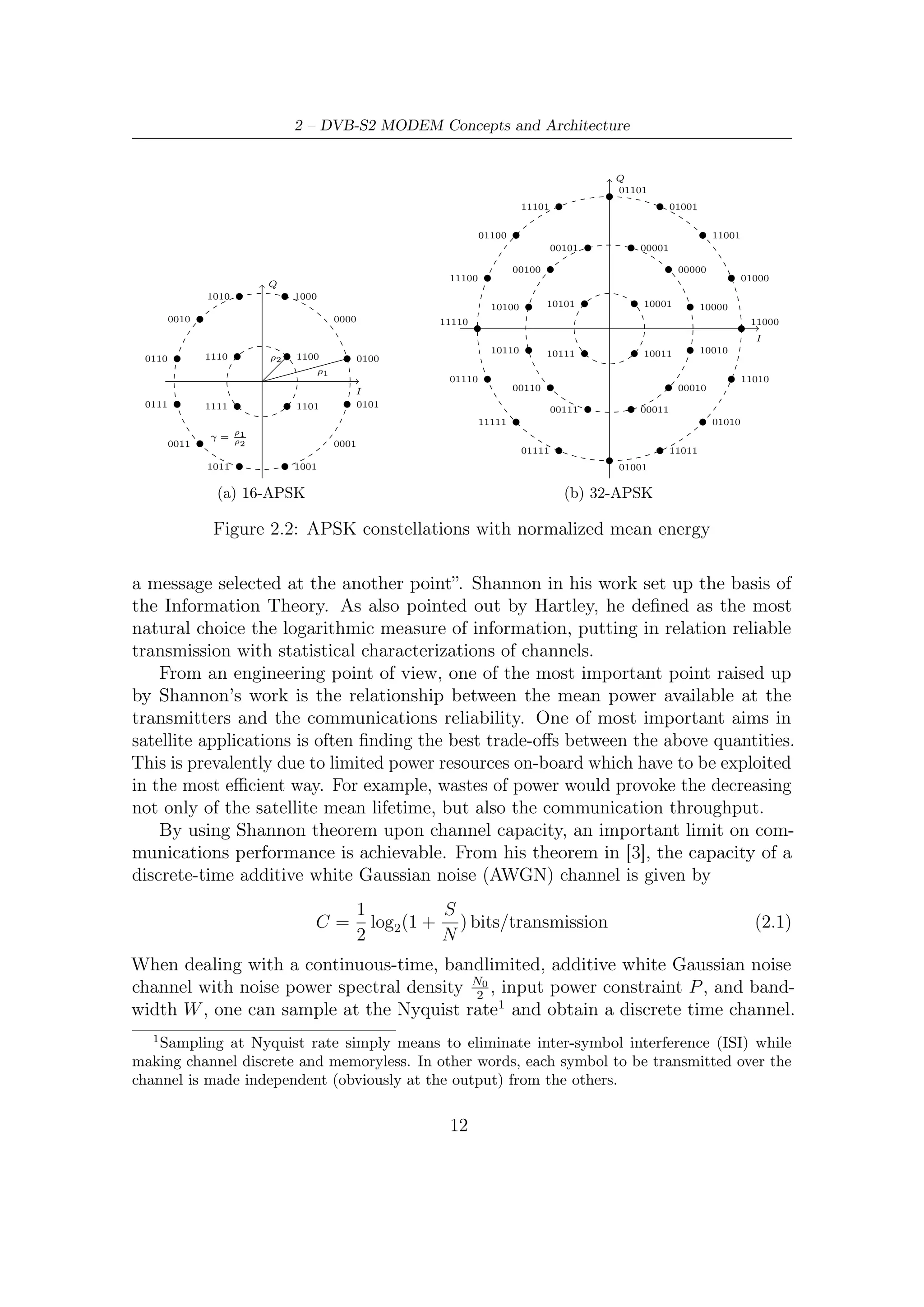
(a) 16-APSK (b) 32-APSK
Figure 2.2: APSK constellations with normalized mean energy
a message selected at the another point”. Shannon in his work set up the basis of
the Information Theory. As also pointed out by Hartley, he defined as the most
natural choice the logarithmic measure of information, putting in relation reliable
transmission with statistical characterizations of channels.
From an engineering point of view, one of the most important point raised up
by Shannon’s work is the relationship between the mean power available at the
transmitters and the communications reliability. One of most important aims in
satellite applications is often finding the best trade-offs between the above quantities.
This is prevalently due to limited power resources on-board which have to be exploited
in the most efficient way. For example, wastes of power would provoke the decreasing
not only of the satellite mean lifetime, but also the communication throughput.
By using Shannon theorem upon channel capacity, an important limit on com-
munications performance is achievable. From his theorem in [3], the capacity of a
discrete-time additive white Gaussian noise (AWGN) channel is given by
1 S
C= log2 (1 + ) bits/transmission (2.1)
2 N
When dealing with a continuous-time, bandlimited, additive white Gaussian noise
channel with noise power spectral density N0 , input power constraint P , and band-
2
width W , one can sample at the Nyquist rate1 and obtain a discrete time channel.
1
Sampling at Nyquist rate simply means to eliminate inter-symbol interference (ISI) while
making channel discrete and memoryless. In other words, each symbol to be transmitted over the
channel is made independent (obviously at the output) from the others.
12

22. 2.1 – Modulation and Coding Schemes
The power per sample will be P and the noise power per sample will be W N0 .
Substituting these results in (2.1), we obtain
1 P
C= log2 1 + bits/transmission (2.2)
2 N0 W
If we multiply this result by the number of transmissions per second, which is 2W ,
we obtain the channel capacity in bps
P
C = W log2 1 + bps (2.3)
N0 W
From this result, the basic factors that determine the channel capacity are the channel
bandwidth W , the noise power spectrum N0 , and the signal power P . There exists a
tradeoff between P and W in the sense that one can compensate for the other.
Increasing the input signal power obviously increases the channel capacity, because
when one has more power to spend, one can choose a larger number of input levels
that are far apart, and therefore more information bits per transmission are possible.
However, the increase in capacity as a function of power is logarithmic and slow.
This is because if one is transmitting with a certain level of immunity against noise
and wants to increase the number of input levels, one has to introduce new levels
with amplitudes higher than the existing levels, and this requires a lot of power. This
fact notwithstanding, the capacity of the channel can be increased to any value by
increasing the input power.
The effect of the channel bandwidth, however, is quite different. Increasing W
has two contrasting effects. On one hand, on a higher bandwidth channel one can
transmit more samples per second and therefore increase the transmission rate. On
the other hand, a higher bandwidth means higher input noise to the receiver and this
degrades its performance. Letting the bandwidth W tend to infinity, one can observe
that, contrary to the power case, capacity can not be increased to any desired value
by increasing the bandwidth alone.
In any practical communication system we must have R < C. If an AWGN
channel is employed, we have
P
R < W log2 1 + (2.4)
N0 W
R
By dividing both sides by W and defining η = W
, the spectral efficiency measured
in bit , we obtain
Hz
P
η < log2 1 + (2.5)
N0 W
13

23. 2 – DVB-S2 MODEM Concepts and Architecture
P
If Eb is the energy per bit, then Eb = R
. By substituting in the previous relation,
we obtain2
Eb
η < log2 1 + η (2.6)
N0
This relation is plotted in Figure 2.3. The curve defined by
Eb 2η − 1
= log10 (2.7)
N0 η
divides the plane in two regions. In one region (above the curve) reliable communi-
cation is possible, and in the other region (below the curve) reliable communication
is not possible. The performance of any communication system can be denoted
by a point in this plane and the closer the point is to this curve, the closer is the
performance of the system to an optimal system. From this curve it is seen that
Eb
= ln 2 = 0,693 ∼ −1,592 dB (2.8)
N0
is an absolute minimum for reliable communication. In other words, for reliable
communications, we must have
Eb
> 0,693 (2.9)
N0
In Figure 2.3, when η 1, we are dealing with a case where bandwidth is large
and the main concern is limitation on power. This case is usually referred to as the
power limited case. Signaling schemes with high dimensionality, such as orthogonal,
biorthogonal, and simplex, are frequently used in these cases. The case, where η 1
happens when the bandwidth of the channel is small, and therefore is referred to
as the bandwidth limited case. Low-dimensional signaling schemes with crowded
constellations are implemented in this case.
Plotting on the spectral efficiency–average power plane performance of several
modulation schemes, we could observe that the SNR penalty (referred to Shannon
limit) decreases with increasing of the modulation order M . In other words, at the
expense of a higher complexity, performance very close to Shannon limit can be
achieved. However, in this manner, the system would operate at spectral efficiencies
excessively small or big if compared to those commonly required.
As we shall see in details in Section 2.4, Figure 2.14 shows performance for each
modulation and coding (C/M) scheme adopted by DVB-S2 modulator with respect
2
If we define W as the the equivalent noise bandwidth on the Nyquist shaping filter, which is
typically chosen in communications to eliminate ISI contribution, we obtain independently from
any roll-off factor that W = Rb . Note that, in fact, for the specific symmetry of Nyquist pulse the
equivalent noise bandwidth on this pulse does not change with roll-off factor variations. Hence the
N0 W
E
reason of simplification Eb Rb = Nb made in this relation.
0
14

24. 2.1 – Modulation and Coding Schemes
100
Bandwidth limited
Signal-to-Noise-Ratio Eb /N0 80
Power limited
60
40
20
0 −1.6 dB
10−2 10−1 100 101
Sprectral efficiency η = Rb /W
Figure 2.3: Shannon Bound: On the horizontal axis is reported spectral efficiency η,
on the vertical axis Signal-to-Noise Ratio measured in dB; Dotted line at −1.6 dB
represents the asymptotic value for η 0; Heavy line is the Shannon curve above
which every point must stays
to the calculated Shannon limit. Thanks to an optimized choice on C/M schemes,
the DVB-S2 modulator provides a wide range of spectral efficiencies (see Table 2.7)
while ensuring performance very close to the Shannon limit.
2.1.4 Adaptive Coding Modulation
Adaptive Coding Modulation (ACM) technique allows different modulation formats
and error protection levels (i.e. coding rates) to be used and changed on a frame-
by-frame basis within the transmitted data stream. By means of a return channel,
informing the transmitter of the actual receiving condition, the transmission parame-
ters may be optimized for each individual user, dependant on link conditions. Today
ACM is considered as a powerful tool to further increase system capacity, allowing
for better utilization of transponder resources.
Since it well-known that the higher the frequency bands used, the less the
link performance tends to remain location-independent and stationary (i.e. stable
space wise), countermeasures to counteract the above link variations are required.
One can adopt static or dynamic solution: adopting static countermeasures against
propagation effects simply means to dimension link parameters (e.g. antenna diameter,
15

25. 2 – DVB-S2 MODEM Concepts and Architecture
power) on worst case basis (link budgets usually contain an item called ‘propagation
margin at nn % of time’); on the other hand, the most common form of dynamic
countermeasure is power control, a technique to manage both propagation phenomena.
Despite the beneficial power control effect on system efficiency, when for instance a
user up-link operates in clear weather or in light of traffic conditions, the potentiality
of that link is not fully exploited. In other words power control helps, but does not
solve to the problem of system parameters over-sizing.
Current point-to-point multi-beam satellite systems based on the DVB-S standard
are designed for link closure in the worst-case propagation and location conditions.
The old DVB-S standard, envisaged for broadcasting applications, considers a fixed
coding rate and modulation format, which are selected according to the assumed
coverage and availability requirements. This approach implies the necessity of high
margins in the majority of the cases, when interference and propagation conditions
allow for higher Signal to Interference plus Noise Ratio (SNIR). Typical Ku-band
broadcasting links are designed with a clear-sky margin of 4 dB to 6 dB and a service
availability target of about 99% of the worst month (or 99,6% of the average year).
Since the rain attenuation curves are very steep in the region 99% to 99,9% of the
time, many dBs of the transmitted satellite power are useful, in a given receiving
location, for only some ten minutes per year. Unfortunately, this waste of satellite
power/capacity cannot be easily avoided for broadcasting services, where millions
of users, spread over very large geographical areas, receive the same content at the
same time.
However, this design methodology, devised for broadcasting systems, is not
optimal for unicast networks. In fact, the point-to-point nature of link connections
allows exploiting spatial and temporal variability of end-user channel conditions for
increasing average system throughput. This is achieved by adapting coding rate and
modulation format (ACM) to best match the user SNIR, thus making the received
data rate location and time dependent. Fixed link margins are therefore avoided and
a remarkable improvement in system capacity is obtained thanks to better utilization
of system power resources.
Assuming a fixed beam power allocation, the key parameters responsible for
SNIR variability within the satellite coverage are the fading attenuation, the satellite
antenna gain and the antenna C/I. The fading attenuation variation is due to
both geographical dependency of rain statistics and to propagation channel time
variations.
One of the key factors, which can heavily affect capacity, is the granularity
of physical layer schemes supported by the system. It is important to ensure a
reasonably small step in Es /N0 and spectral efficiency between consecutive schemes
in order to maximize the data rate provided to STs. In particular, it is of the highest
importance for capacity purposes utilizing a sufficiently fine granularity in the SNIR
range experienced in the coverage during clear sky conditions. On the contrary,
16

26. 2.2 – ACM Modem System Description
larger SNIR intervals can be assumed between the more robust modes without major
capacity penalty, due to their lower occurrence probability.
The DVB-S2 ACM modulator operates at constant symbol rate, since the available
transponder bandwidth is assumed constant. ACM is implemented by the DVB-
S2 modulator by transmitting a TDM sequence of physical layer frames, each
transporting a coded block and adopting a uniform modulation format. However,
when ACM is implemented, coding scheme and modulation format may change frame-
by-frame. Therefore service continuity is achieved, during rain fades, by reducing
user bits while increasing at the same time FEC redundancy and/or modulation
ruggedness.
ACM technique therefore allows to significantly increase the average system
throughput and availability of satellite networks, thus making the system economically
more attractive for interactive applications. The increase is mainly dependant on
the adopted frequency band, target link and service area availability requirements
and related system sizing options. Compared to Constant Coding and Modulation
(CCM), an ACM-based system can provide:
• higher system throughput than the one supported by a CCM system, as an
ACM system can take benefit from better link propagation and beam C/I
conditions than the worst case link on which CCM physical layer is sized;
• higher availability (time-link and/or spatial) than the one supported by the
CCM system as when deeper fading occurs the ACM system can use a more
robust modulation and coding scheme. This is obtained through a very small
reduction of the total system throughput as the number of users affected by
these deep fade events is very limited. The highest link availability and service
area supported by the system depends on the lowest modulation and coding
scheme supported by the system;
• more optimization dimensions in the system design to cope with more pushed
frequency reuse and more complex satellite antennas.
2.2 ACM Modem System Description
DVB-S2 ACM Modem system is defined as the functional block of equipment
performing the adaptation of the baseband digital signals, from the output of a single
(or multiple) MPEG transport stream multiplexer(s), or from the output of a single
(or multiple) generic data source(s), to the satellite channel characteristics. Data
services may be transported in Transport Stream format (e.g. using Multi-protocol
Encapsulation3 ) or Generic Stream format.
3
It is a means to allow more than a packet format (e.g., IP) over MPEG frames.
17

27. 2 – DVB-S2 MODEM Concepts and Architecture
If the received signal is above the C/N +I threshold, the Forward Error Correction
(FEC) technique adopted in the System is designed to provide a ‘Quasi Error Free’
(QEF) quality target. The definition of QEF adopted for DVB-S2 is “less than one
uncorrected error-event per transmission hour at the level of a 5 Mbit/s single TV
service decoder”, approximately corresponding to a Transport Stream Packet Error
Ratio PER < 10−7 before de-multiplexer.
2.2.1 Architecture and Sub-Blocks Specifications
According to Figure 2.4, the DVB-S2 System is composed of a sequence of functional
blocks as described below.
Mode Adaptation is application dependent. It provides input stream interfacing,
Input Stream Synchronization (optional), null-packet deletion (for ACM and
Transport Stream input format only), CRC-8 coding for error detection at
packet level in the receiver (for packetized input streams only), merging of
input streams (for Multiple Input Stream modes only) and slicing into DATA
FIELDs. For Constant Coding and Modulation (CCM) and single input
Transport Stream, Mode Adaptation consists of a ‘transparent’ DVB-ASI (or
DVB-parallel) to logical-bit conversion and CRC-8 coding.
A Base-Band Header is appended in front of the Data Field, to notify the
receiver of the input stream format and Mode Adaptation type. To be noted
that the MPEG multiplex transport packets may be asynchronously mapped
to the Base-Band Frames.
Stream Adaptation is applied to provide padding to complete a Base-Band Frame
and Base-Band Scrambling.
Forward Error Correction (FEC) Encoding is carried out by the concatena-
tion of BCH outer codes and LDPC (Low Density Parity Check) inner codes
(rates 1/4, 1/3, 2/5, 1/2, 3/5, 2/3, 3/4, 4/5, 5/6, 8/9, 9/10). Depending on
the application area, the FEC coded blocks have length nldpc = 64800 bits
or 16 200 bits. When VCM and ACM is used, FEC and modulation mode
may be changed in different frames, but remains constant within a frame. Bit
interleaving is applied to FEC coded bits for 8PSK, 16APSK and 32APSK.
Mapping into QPSK, 8PSK, 16APSK and 32APSK constellations is applied, de-
pending on the application area. Gray mapping of constellations is used for
QPSK and 8PSK.
Physical Layer Framing Physical layer framing should be applied, synchronous
with the FEC frames, to provide Dummy PLFRAME insertion, Physical
18

28. 2.2 – ACM Modem System Description
Layer (PL) Signalling, pilot symbols insertion (optional) and Physical Layer
Scrambling for energy dispersal. Dummy PLFRAMEs are transmitted when no
useful data is ready to be sent on the channel. The System provides a regular
physical layer framing structure, based on SLOTs of M = 90 modulated symbols,
allowing reliable receiver synchronization on the FEC block structure. A slot is
devoted to physical layer signalling, including Start-of-Frame delimitation and
transmission mode definition. This mechanism is suitable also for VCM and
ACM demodulator setting. Carrier recovery in the receivers may be facilitated
by the introduction of a regular raster of pilot symbols (P = 36 pilot symbols
every 16 SLOTs of 90 symbols), while a pilot-less transmission mode is also
available, offering an additional 2,4% useful capacity.
Base-Band Filtering and Quadrature Modulation is applied to shape the sig-
nal spectrum (squared-root raised cosine, roll-off factors 0,35 or 0,25 or 0,20)
and to generate the RF signal.
Figure 2.4: Functional block diagram of DVB-S2 ACM modem architecture
2.2.2 Sub-Blocks Description
The following subsystems description is organized according to the functional block
diagram in Figure 2.4.
19

29. 2 – DVB-S2 MODEM Concepts and Architecture
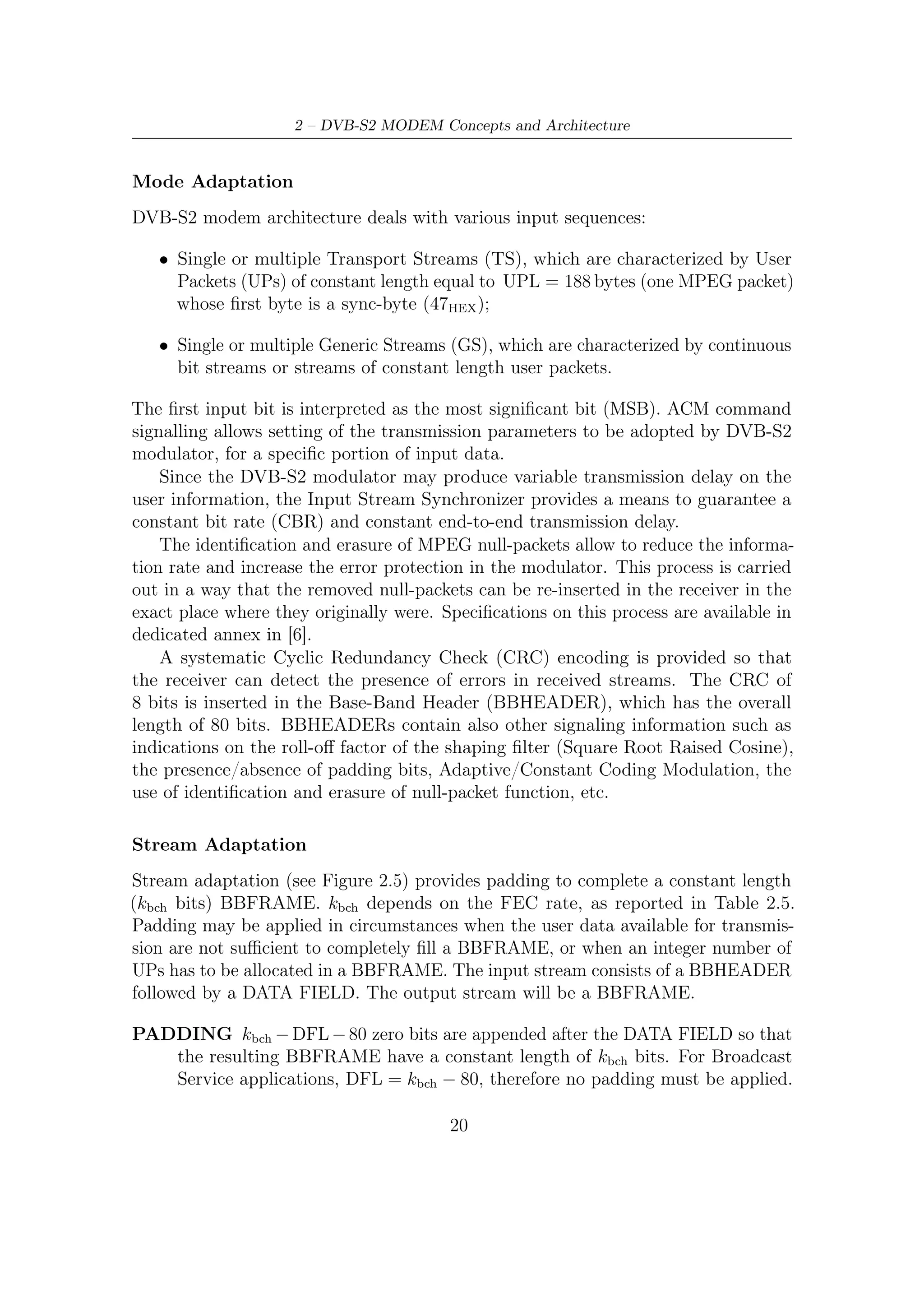
Mode Adaptation
DVB-S2 modem architecture deals with various input sequences:
• Single or multiple Transport Streams (TS), which are characterized by User
Packets (UPs) of constant length equal to UPL = 188 bytes (one MPEG packet)
whose first byte is a sync-byte (47HEX );
• Single or multiple Generic Streams (GS), which are characterized by continuous
bit streams or streams of constant length user packets.
The first input bit is interpreted as the most significant bit (MSB). ACM command
signalling allows setting of the transmission parameters to be adopted by DVB-S2
modulator, for a specific portion of input data.
Since the DVB-S2 modulator may produce variable transmission delay on the
user information, the Input Stream Synchronizer provides a means to guarantee a
constant bit rate (CBR) and constant end-to-end transmission delay.
The identification and erasure of MPEG null-packets allow to reduce the informa-
tion rate and increase the error protection in the modulator. This process is carried
out in a way that the removed null-packets can be re-inserted in the receiver in the
exact place where they originally were. Specifications on this process are available in
dedicated annex in [6].
A systematic Cyclic Redundancy Check (CRC) encoding is provided so that
the receiver can detect the presence of errors in received streams. The CRC of
8 bits is inserted in the Base-Band Header (BBHEADER), which has the overall
length of 80 bits. BBHEADERs contain also other signaling information such as
indications on the roll-off factor of the shaping filter (Square Root Raised Cosine),
the presence/absence of padding bits, Adaptive/Constant Coding Modulation, the
use of identification and erasure of null-packet function, etc.
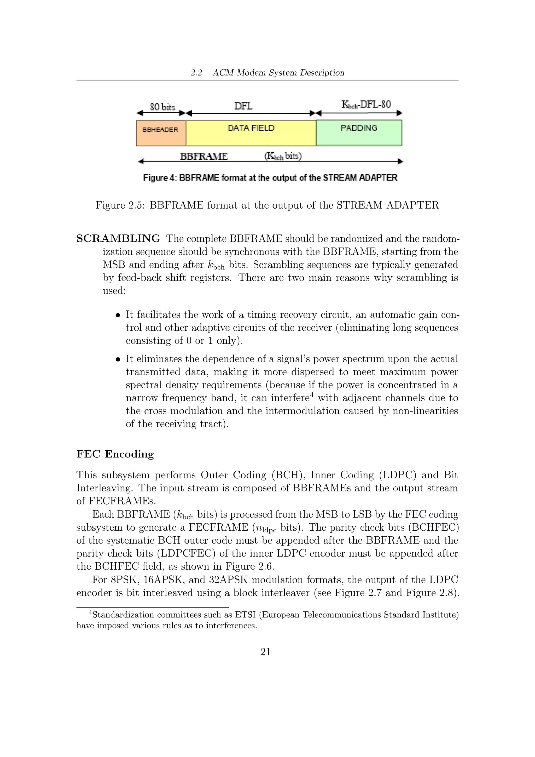
Stream Adaptation
Stream adaptation (see Figure 2.5) provides padding to complete a constant length
(kbch bits) BBFRAME. kbch depends on the FEC rate, as reported in Table 2.5.
Padding may be applied in circumstances when the user data available for transmis-
sion are not sufficient to completely fill a BBFRAME, or when an integer number of
UPs has to be allocated in a BBFRAME. The input stream consists of a BBHEADER
followed by a DATA FIELD. The output stream will be a BBFRAME.
PADDING kbch − DFL − 80 zero bits are appended after the DATA FIELD so that
the resulting BBFRAME have a constant length of kbch bits. For Broadcast
Service applications, DFL = kbch − 80, therefore no padding must be applied.
20

30. 2.2 – ACM Modem System Description
Figure 2.5: BBFRAME format at the output of the STREAM ADAPTER
SCRAMBLING The complete BBFRAME should be randomized and the random-
ization sequence should be synchronous with the BBFRAME, starting from the
MSB and ending after kbch bits. Scrambling sequences are typically generated
by feed-back shift registers. There are two main reasons why scrambling is
used:
• It facilitates the work of a timing recovery circuit, an automatic gain con-
trol and other adaptive circuits of the receiver (eliminating long sequences
consisting of 0 or 1 only).
• It eliminates the dependence of a signal’s power spectrum upon the actual
transmitted data, making it more dispersed to meet maximum power
spectral density requirements (because if the power is concentrated in a
narrow frequency band, it can interfere4 with adjacent channels due to
the cross modulation and the intermodulation caused by non-linearities
of the receiving tract).
FEC Encoding
This subsystem performs Outer Coding (BCH), Inner Coding (LDPC) and Bit
Interleaving. The input stream is composed of BBFRAMEs and the output stream
of FECFRAMEs.
Each BBFRAME (kbch bits) is processed from the MSB to LSB by the FEC coding
subsystem to generate a FECFRAME (nldpc bits). The parity check bits (BCHFEC)
of the systematic BCH outer code must be appended after the BBFRAME and the
parity check bits (LDPCFEC) of the inner LDPC encoder must be appended after
the BCHFEC field, as shown in Figure 2.6.
For 8PSK, 16APSK, and 32APSK modulation formats, the output of the LDPC
encoder is bit interleaved using a block interleaver (see Figure 2.7 and Figure 2.8).
4
Standardization committees such as ETSI (European Telecommunications Standard Institute)
have imposed various rules as to interferences.
21

31. 2 – DVB-S2 MODEM Concepts and Architecture
Figure 2.6: Format of data before Bit Interleaving
Data is serially written into the interleaver column-wise, and serially read out row-
wise (the MSB of BBHEADER is read out first, except 8PSK rate 3/5 case where
MSB of BBHEADER is read out third) as shown in the figures.
Figure 2.7: Bit Interleaving scheme for 8PSK (for each rate except from 3/5) and
normal FECFRAME length
Bit Mapping
Each FECFRAME (which is a sequence of 64800 bits for normal FECFRAME, or
16200 bits for short FECFRAME), must be serial-to-parallel converted (parallelism
22

32. 2.2 – ACM Modem System Description
Figure 2.8: Bit Interleaving scheme for 8PSK (rate 3/5) and normal FECFRAME
length
Modulation Rows (n = 64800) Rows (n = 16200) Columns
8PSK 21600 5400 3
16APSK 16200 4050 4
32APSK 12960 3240 5
Table 2.1: Bit Interleaver structure
level ηMOD = 2 for QPSK, 3 for 8PSK, 4 for 16APSK, 5 for 32APSK) in figures 9
to 12, the MSB of the FECFRAME is mapped into the MSB of the first parallel
sequence. Each parallel sequence shall be mapped into constellation, generating a
(I,Q) sequence of variable length depending on the selected modulation efficiency
ηMOD .
The input sequence is a FECFRAME, the output sequence is a XFECFRAME
64800 16200
(compleX FECFRAME), composed of ηMOD (normal XFECFRAME) or ηMOD (short
XFECFRAME) modulation symbols. Each modulation symbol is a complex vector in
the format (I,Q) (I being the in-phase component and Q the quadrature component)
or in the equivalent format ρ exp(jφ)(ρ being the modulus of the vector and φ being
its phase).
For QPSK, the System employs conventional Gray-coded QPSK modulation with
absolute mapping (no differential coding). Bit mapping into the QPSK constellation
23

33. 2 – DVB-S2 MODEM Concepts and Architecture
is illustrated in Figure 2.1. The normalized average energy per symbol is equal to
ρ2 = 1. Two FECFRAME bits are mapped to a QPSK symbol, i.e. bits 2i and 2i + 1
determines the i-th QPSK symbol, where i = 0, 1, 2, . . . , (N/2) − 1 and N is the
coded LDPC block size.
For 8PSK, the System employs conventional Gray-coded 8PSK modulation with
absolute mapping (no differential coding). Bit mapping into the 8PSK constellation
is shown in Figure 2.1. The normalized average energy per symbol is equal to ρ2 = 1.
For all the rates excluding 3/5, bits 3i, 3i+1, 3i+2 of the interleaver output determine
the ith 8PSK symbol where i = 0, 1, 2, . . . , (N/3) − 1and N is the coded LDPC block
size. For rate 3/5 bits 3i + 2, 3i + 1, 3i of the interleaver output determine the i-th
8PSK symbol where I = 0, 1, 2, . . . , (N/3) − 1 and N is the coded LDPC block size.
The 16APSK modulation constellation (see figure Figure 2.1) is composed of two
concentric rings of uniformly spaced 4 and 12 PSK points, respectively in the inner
ring of radius ρ1 and outer ring of radius ρ2 . The ratio of the outer circle radius to the
inner circle radius (γ = ρ2 /ρ1 ) should be comply with Table 2.3. If 4ρ1 2 + 12ρ2 2 = 16
the average signal energy becomes 1. Bits 4i,4i + 1,4i + 2 and 4i + 3 of the interleaver
output determine the i-th 16APSK symbol, where i = 0, 1, 2, . . . , (N/4) − 1 and N
is the coded LDPC block size.
The 32APSK modulation constellation (see Figure 2.1) is composed of three
concentric rings of uniformly spaced 4, 12 and 16 PSK points, respectively in the inner
ring of radius ρ1 , the intermediate ring of radius ρ2 and the outer ring or radius ρ3 .
Table 2.2 defines the values of γ1 = ρ2 /ρ1 and γ2 = ρ3 /ρ1 . If 4ρ1 2 +12ρ2 2 +16ρ3 2 = 32
the average signal energy becomes equal to 1. Bits 5i, 5i + 1, 5i + 2, 5i + 3 and 5i + 4 of
the interleaver output determine the i-th 32APSK symbol, where i = 0, 1, 2, (N/5)−1.
Code Rate η γ1 γ2
3/4 3,74 2,84 5,27
4/5 3,99 2,72 4,87
5/6 4,15 2,64 4,64
8/9 4,43 2,54 4,33
9/10 4,49 2,53 4,3
Table 2.2: Optimum constellation radius ratios γ1 and γ2 (linear channel) for 32APSK
Physical Layer (PL) Framing
This block generates, synchronously with FECFRAMEs, physical layer frames (PL-
FRAMEs) and deal with
• the insertion of physical headers and optional pilot symbols (their insertion
causes a loss of 2,4% of capacity);
24

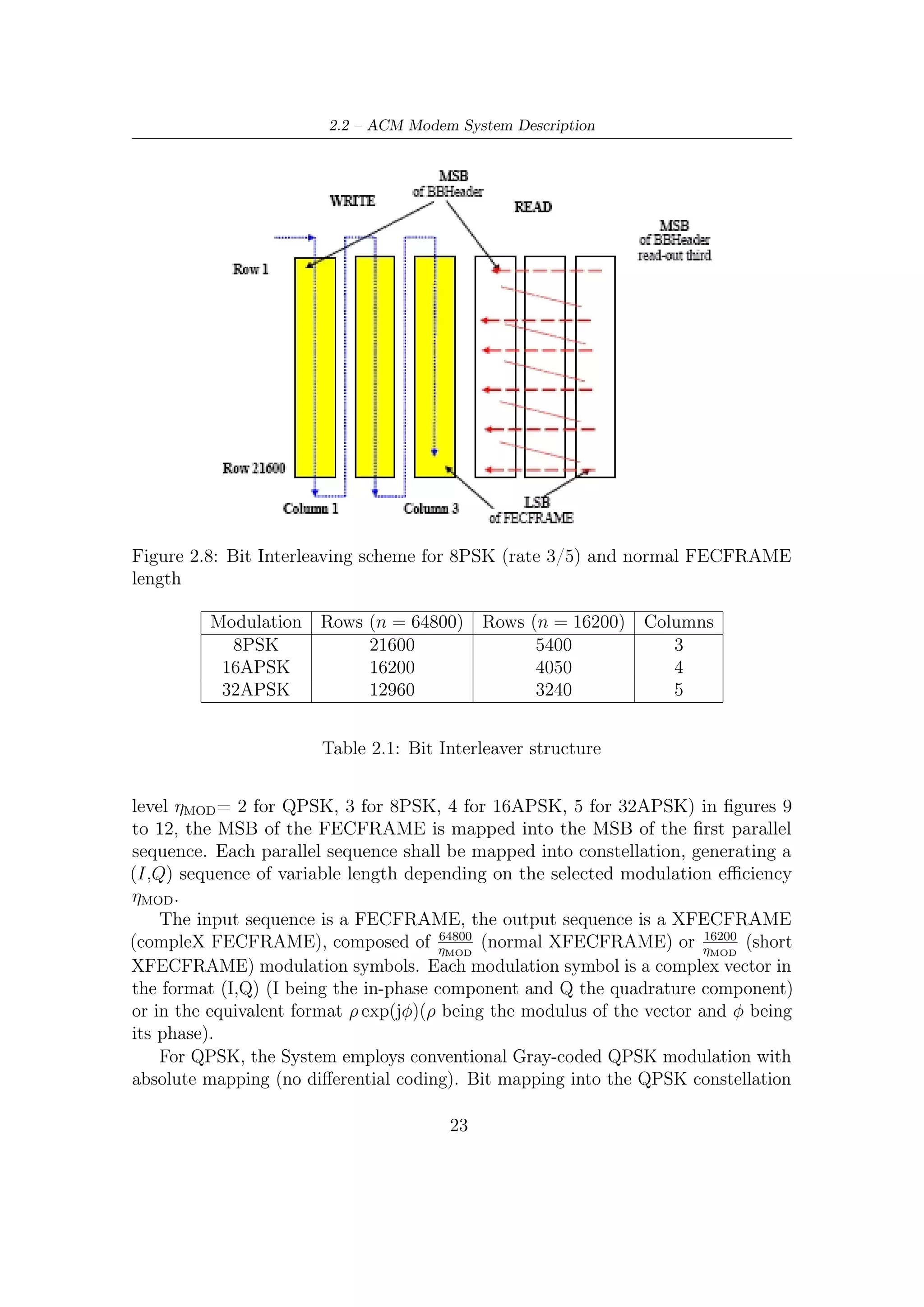
34. 2.3 – Inner and Outer FEC
Code Rate η γ
2/3 2,66 3,15
3/4 2,99 2,85
4/5 3,19 2,75
5/6 3,32 2,7
8/9 3,55 2,6
9/10 3,59 2,57
Table 2.3: Optimum constellation radius ratio γ (linear channel) for 16APSK
• the insertion of dummy frames to be used in absence of data ready to be
immediately transmitted;
• the scrambling (or the randomization) for energy dispersal by multiplying the
(I + j Q) samples by a complex radomization sequence (CI + j CQ ).
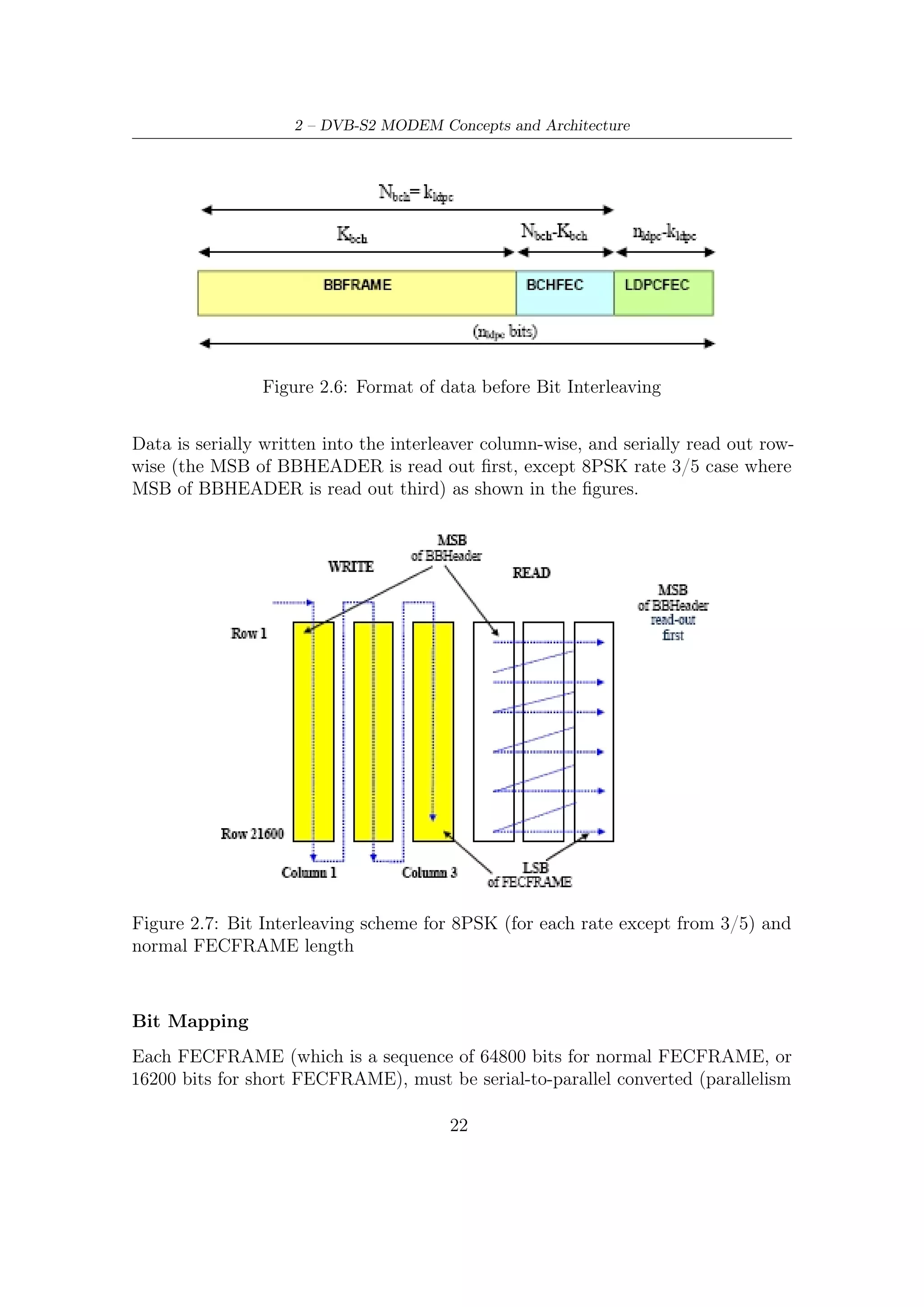
2.3 Inner and Outer FEC
The DVB-S2 FEC section relies on two block codes concatenation, i.e., codewords
generated by BCH encoder are, in turn, encoded by LDPC encoder5 . Thus, BCH
code is usually called outer code and LDPC inner code. Outputs from FEC encoding
section are formatted according to Figure 2.6. As we shall see later on, this BCH
concatenation gives an extra protection [6] against unwanted error floors at high
SNR6 When the decoding has to be performed, the above sequence of encoding
steps must be, of course, inverted: in other words, LDPC starts to decode prior to
BCH. As just said, error floor phenomena at high signal-to-noise ratio typically affect
the decoding performance, and therefore the BCH extra protection against residual
5
Note that each frame (either short or long) is processed from most significant to least significant
bit, either by BCH or LDPC.
6
The iterative decoding achieves very close to Shannon limit performance at low/medium SNR.
On the contrary, its performance may be significantly worse at high SNR. In fact, their free distance
(the minimum Hamming distance between different codewords, i.e., the minimum Hamming weight
of a nonzero codeword) can be low. This causes BER curve to flatten following the error floor tied
to dfree , after the waterfall region at low SNR. Performance of any binary code at high SNR can be
well approximated by the expression of union bound, truncated to the contribution of free distance
(terms at higher distance are negligible at high SNR). Such expression [18] is
1 wfree k Eb
BER erfc dfree
2 k n N0
25

35. 2 – DVB-S2 MODEM Concepts and Architecture
errors is aimed at counteracting to the performance degradation, enhancing FEC
robustness at higher SNR.
In a some sense, the chain constituted, in order, by LDPC encoder, channel and
LDPC decoder can be conceived as a super-channel on which BCH encoder/decoder
operates. This kind of intuitive representation puts in evidence the advantage of
concatenating two codes. The best choices on their kind of concatenation can give a
powerful tool to enhance the performance of the overall FEC decoding, allowing to
act by a outer coding on the weaknesses of the inner coding.
2.3.1 BCH
BCH code is named for Bose, Ray-Chaudhury, and Hocquenghem, who published
work in 1959 and1960 which revealed a means of designing codes over GF (2) with
a specified design distance. BCH codes are cyclic codes and thus, as explained in
Appendix B, can be specified by a generator polynomial. In present Section we
give only some notations over the particular, as we shall see, structure of BCH code
employed in DVB-S2 and, more generally, over its design steps.
A BCH code of length n with a specified minimum distance, or, i.e., capable of
correcting (at least) t errors, can be designed as follows [15, 9]:
1. Determine the smallest m such that GF (q m ) has primitive nth root (Section
A.5) of unity β.
2. Select a nonnegative integer b. In most of cases, it is selected b = 1.
3. Write down a list of 2t consecutive powers of β (see Section A.3):
β b , β b+1 , . . . , β b+2t−1
Determine the minimal polynomial of each of these powers of β. (Because of
conjugacy, frequently these minimal polynomials are not distinct.)
4. The generator polynomial g(x) is least common multiple (LCM) of these
minimal polynomials. The code is a (n, n − deg(g(x))) cyclic code.
Two fields are involved in the construction of the BCH codes. The small field
GF (q) is where the generator polynomial has its coefficients and is the field where the
elements of the codeword are. The big field GF (q m ) is the field where the generator
polynomial has its roots. For encoding purposes it is only sufficient to have the
polynomial generator of the code, whereas, for decoding, the additionally knowledge
of the extension field where the generator has its roots is necessary. Two definitions
will be useful later on: first, if β selected is a primitive element then the code is
called primitive; second, when β = 1 the code is said to be a code in narrow-sense.
26

36. 2.3 – Inner and Outer FEC
It can be proved that following the constructive procedure described above
produces codes with at least the specified minimum distance. As shown in Appendix
B, since every codeword is a multiple of the generator polynomial, we can express
the parity check condition as follows
c(β i ) = m(β i )g(β i ) = m(β i ) · 0 (2.10)
for i = b, b + 1, . . . , b + 2t − 1. In fact these powers of β are, by design, the roots of
g(x). Rewriting these condition using the correspondent vector representation we
get the following system of equations
n−1
c0 + c1 β i + c2 β i+1 + . . . + cn−1 (β i ) =0 (2.11)
always for i = b, b + 1, . . . , b + 2t − 1. Therefore 2t parity check conditions can be
also expressed in the matrix form
 
c0
 c1 
 
1 β i β 2i · · · β (n−1)i  c2  = 0 (2.12)
 
 . .
 . 
cn−1
Stacking the row vectors for different values of i we get the following parity check
matrix  
1 βb β 2b ... β (n−1)b
 1 β b+1 β 2(b+1) . . . β (n−1)(b+1) 
 
 .
 . (2.13)

 .

b+δ−3 2(b+δ−3) (n−1)(b+δ−3) 

 1 β β ... β
b+δ−2 2(b+δ−2)
1 β β . . . β (n−1)(b+δ−2)
where δ = 2t + 1 represent the design distance (Hamming metric) of the code.
It can be proved (see [15]) that the matrix H have at least δ = 2t + 1 columns
linearly dependent and, thus, the minimum distance of the code satisfies dmin ≥ δ;
that is, the code is capable of correcting at least t errors.
In DVB-S2 context, BCH outer code has been designed to avoid “unpredictable
and unwanted error floors which affect iterative decodings at high C/N ratios”, i.e.,
at low bit error rates (BER).
Although the mathematical background shown in this thesis in order to design,
encoding and decoding is completely general, in the most practical cases the base
fields of BCH codes is GF (2), as in DVB-S2 FEC section. The polynomials which
must be multiplied in order to obtain the wanted BCH code associated to a specific
operating mode (or, i.e., error correction capability) are shown in Table 2.4. More
27

37. 2 – DVB-S2 MODEM Concepts and Architecture
specifically, multiplication of the first t of them provides a polynomial generator of
the BCH code capable of correcting at least t error. Notice that this procedure is in
accordance with the third step to construct generator polynomial of the BCH code.
The encoding suggestions, provided in [6], are typical of a cyclic codes in system-
atic form, whose specific properties and encoding steps are discussed in dedicated
Appendix B. It is worth understanding that both systematic and non-systematic
codewords are always multiple of the generator polynomial of the code (or, i.e., of
the ideal, as also shown in Section B.2) so that parity check condition (2.12) is still
valid as well as BCH bound. Furthermore, from a direct analysis of the polynomial
supplied by [6] (Normal FEC-Frame), one could observe that these specific codes
(one for each selected error protection level) are primitive and, indeed, narrow-sense.
The reasons are described in the following
• g1 (x) is one of the possible primitive polynomial which has its roots in GF (216 ).
16
This can be quickly proved verifying that α2 −1 = 1 by computer aid or, more
lazily, by direct consultation of any table of primitive polynomials. For the
tables of primitive polynomials, the interested reader could refer to [21]
• Hence, this BCH is a narrow-sense code. In fact, by design, it follows that b
must be equal to 1.
Three different t-error correcting BCH codes (t = 12, t = 10, t = 8) should be
applied to each BBFRAME, according to LDPC coding rates as shown in Table 2.5.
Outer FEC (i.e. BCH), although there are 11 LDPC coding rates, deal with only
three different error protection level: t = 12, t = 10, t = 8. On the one hand we have,
since this BCH is primitive, that the codeword length must be equal to 216 − 1. On
the other hand we have in Table 2.5 multiple codeword lengths for each t-BCH code
and all of them do not correspond to the primitive length BCH should have. In
general, for each code rate, a different set of polynomials to be multiplied would be
expected, whereas, in DVB-S2, there is only one set of polynomials provided by [6].
Eventually, we have to conclude that DVB-S2 BCH code is shortened. A system-
atic (n, k) code can be shortened by setting a number of the information bits to zero
(i.e, zero padding). This means that a linear (n, k) code consisting of k information
bits and n − k check bits (or redundancy bits) can be shortened into a (n − l, k − l)
linear code by setting the most (or the least, depending on the reference direction)
significant first l bits to zero. As also described in [15], shortening of a code does
not have bad effects on its minimum distance properties and its decoding algorithms.
However, shortened cyclic code might loose its cyclic property.
28

38. 2.3 – Inner and Outer FEC
g1 (x) 1 + x2 + x3 + x5 + x16
g2 (x) 1 + x + x4 + x5 + x6 + x8 + x16
g3 (x) 1 + x2 + x3 + x4 + x5 + x7 + x8 + x9 + x10 + x11 + x16
g4 (x) 1 + x2 + x4 + x6 + x9 + x11 + x12 + x14 + x16
g5 (x) 1 + x + x2 + x3 + x5 + x8 + x9 + x10 + x11 + x12 + x16
g6 (x) 1 + x2 + x4 + x5 + x7 + x8 + x9 + x10 + x12 + x13 + x14 + x15 + x16
g7 (x) 1 + x2 + x5 + x6 + x8 + x9 + x10 + x11 + x13 + x15 + x16
g8 (x) 1 + x + x2 + x5 + x6 + x8 + x9 + x12 + x13 + x14 + x16
g9 (x) 1 + x5 + x7 + x9 + x10 + x11 + x16
g10 (x) 1 + x + x2 + x5 + x7 + x8 + x10 + x12 + x13 + x14 + x16
g11 (x) 1 + x + x2 + x3 + x5 + x9 + x11 + x12 + x13 + x16
g12 (x) 1 + x + x5 + x6 + x7 + x9 + x11 + x12 + x16
Table 2.4: BCH minimal polynomials for normal FECFRAME nLDPC = 64800
LDPC Code BCH Uncoded BCH Coded BCHFEC BCH t-error
Rate Block Block Correction
1/4 16008 16200 192 12
1/3 21408 21600 192 12
2/5 25728 25920 192 12
1/2 32208 32400 192 12
3/5 38688 38880 192 12
2/3 43040 43200 160 10
3/4 48408 48600 192 12
4/5 51648 51840 192 12
5/6 53840 54000 160 10
8/9 57472 57600 128 8
9/10 58192 58320 128 8
Table 2.5: Coding parameters for normal FECFRAME nLDPC = 64800
2.3.2 LDPC
LDPC codes [17] were invented in 1960 by R. Gallager. They were largely ignored until
the discovery of turbo codes [2] in 1993. Since then, LDPC codes have experienced a
renaissance and are now one of the most intensely studied areas in coding.
Much of the effort in coding over the last 50 years has focused on the construction
of highly structured codes with large minimum distance. The structure keeps the
decoding complexity manageable, while large minimum distance is supposed to
guarantee good performance. This approach, however, is not without its drawbacks.
First, it seems that finding structured codes with large minimum distance turn
29

39. 2 – DVB-S2 MODEM Concepts and Architecture
out to be a harder problem than researchers imagined. Finding good codes in
general is, in a sense, trivial: randomly chosen codes are good with high probability.
More generally, one can easily construct good codes provided one admits sufficient
description complexity into the definition of the code. This conflicts, however, with
the goal of finding highly structured codes that have simple decodings. Second,
close to capacity, minimum distance is only a poor surrogate for the performance
measure of real interest. Iterative coding systems take an entirely different approach.
The basic idea is the following. Codes are constructed so that the relationship
between their bits (the structure of their redundancy) is locally simple, admitting
simple local decoding. The local descriptions of the codes are interconnected in a
complex (e.g., random- like) manner, introducing long-range relationships between
the bits. Relatively high global description complexity is thereby introduced in the
interconnection between the simple local structures. Iterative decoding proceeds
by performing the simple local decodings and then exchanging the results, passing
messages between locales across the ‘complex’ interconnection. The locales repeat
their simple decodings, taking into account the new information provided to them
from other locales. Usually, one uses a graph to represent this process. Locales are
nodes in the graph, and interconnections are represented as edges. Thus, description
complexity is introduced without adding computational complexity per se, but rather
as wiring or routing complexity.
In addition to the classical representation of block codes (i.e. by H matrix),
another useful and common way of representing an LDPC codes is through a graphical
representation called a Tanner graph [17, 15, 5]. Tanner graphs of LDPC codes
are bipartite graphs with variable nodes on one side and constraint nodes on the
other. Each variable node corresponds to a bit, and each constraint node corresponds
to one parity-check constraint on the bits defining a codeword. A parity-check
constraint applies to a certain subset of the codeword bits, those that participate
in the constraint. The parity-check is satisfied if the XOR of the participating bits
is 0 or, equivalently, the modulo 2 sum of the participating bits is 0. Edges in the
graph attach variable nodes to constraint nodes indicating that the bit associated
with the variable node participates in the parity-check constraint associated with the
constraint node. A bit sequence associated with the variable nodes is a codeword if
and only if all of the parity-checks are satisfied.
The Tanner graph representation of the LDPC code closely mirrors the more
standard parity-check matrix representation of a code. In this latter description
the code is represented as the set of all binary solutions x = (x1 , x2 , . . . , xn ) to a
simple linear algebraic equation (parity check equations [9, 21, 15, 5]) HxT = 0T .
The elements of the parity-check matrix are 0s and 1s, and all arithmetic is modulo
2, that is, multiplication of x by a row of H means taking the XOR of the bits in x
corresponding to the 1s in the row of H. The connection between the parity-check
matrix representation and the Tanner graph is straightforward, and is illustrated
30

40. 2.3 – Inner and Outer FEC
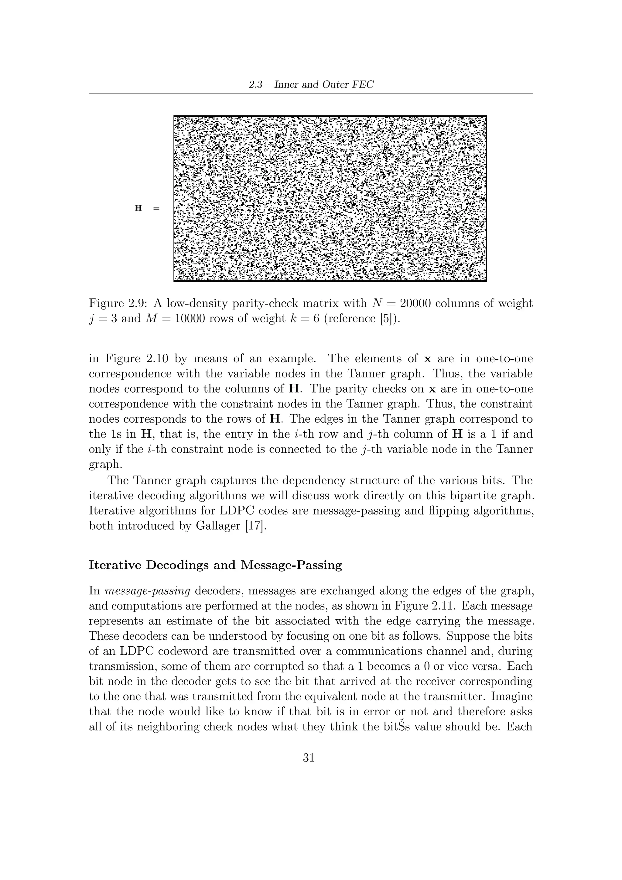
Figure 2.9: A low-density parity-check matrix with N = 20000 columns of weight
j = 3 and M = 10000 rows of weight k = 6 (reference [5]).
in Figure 2.10 by means of an example. The elements of x are in one-to-one
correspondence with the variable nodes in the Tanner graph. Thus, the variable
nodes correspond to the columns of H. The parity checks on x are in one-to-one
correspondence with the constraint nodes in the Tanner graph. Thus, the constraint
nodes corresponds to the rows of H. The edges in the Tanner graph correspond to
the 1s in H, that is, the entry in the i-th row and j-th column of H is a 1 if and
only if the i-th constraint node is connected to the j-th variable node in the Tanner
graph.
The Tanner graph captures the dependency structure of the various bits. The
iterative decoding algorithms we will discuss work directly on this bipartite graph.
Iterative algorithms for LDPC codes are message-passing and flipping algorithms,
both introduced by Gallager [17].
Iterative Decodings and Message-Passing
In message-passing decoders, messages are exchanged along the edges of the graph,
and computations are performed at the nodes, as shown in Figure 2.11. Each message
represents an estimate of the bit associated with the edge carrying the message.
These decoders can be understood by focusing on one bit as follows. Suppose the bits
of an LDPC codeword are transmitted over a communications channel and, during
transmission, some of them are corrupted so that a 1 becomes a 0 or vice versa. Each
bit node in the decoder gets to see the bit that arrived at the receiver corresponding
to the one that was transmitted from the equivalent node at the transmitter. Imagine
that the node would like to know if that bit is in error or not and therefore asks
all of its neighboring check nodes what they think the bitŠs value should be. Each
31

41. 2 – DVB-S2 MODEM Concepts and Architecture
Figure 2.10: A parity check matrix H and the corresponding Tanner graph. To
illustrate the relationship more clearly, some edge are shown in red or blue.
neighboring check node then asks their other neighbors what their bit values are and
sends back to the original bit node the modulo 2 sum of those values. The bit node
now has several opinions as to the bitŠs correct value and must somehow reconcile
these opinions; it could, for example, take a majority vote. The above procedure
constitutes one round or iteration of message passing.
Figure 2.11: The principle of a message-passing decoder. Messages represent an
estimate of the bit associated with the edge carrying the message. Nodes query
neighboring nodes to collect opinions, process this information, and forward their
current estimate to their neighbors.
In order to improve performance, a further such round can be performed. In more
detail, assume that those bit nodes that send their observed bits to the checks to
32

42. 2.3 – Inner and Outer FEC
be summed first ask their check node neighbors what they think is their correct bit
value. Those check nodes could then query their other variable node neighbors and
forwarded their modulo 2 sum as an opinion. With more information now available,
the bit nodes would have a better chance of communicating the correct value to
the check nodes, and the opinions returned to the original node would therefore
have a better chance of being correct. This gathering of opinions could obviously be
extended through multiple iterations; typically, many iteration rounds are performed.
In actual decoding all nodes decode concurrently. Each node gathers opinions
from all its neighbors and forwards to each neighbor an opinion formed by combining
the opinions of the other neighbors. This is the source of the term message passing.
The process continues until either a set of bits is found that satisfies all checks or
time runs out. The message passing may proceed asynchronously. Note that with
LDPC codes, convergence to a codeword is easy to detect since one need only verify
that the parity checks are satisfied.
The processing required for message-passing decoding LDPC codes is highly
parallelizable and flexible. Each message-passing operation performed at a node
depends on other nodes only through the messages that arrive at that node. Moreover,
message updating need not be synchronized. Consequently, there is great freedom
to distribute in time and space the computation required to decode LDPC codes.
Turbo codes are also decoded using belief propagation, but their structure does not
admit the same level of atomization.
There is a second distinct class of decoding algorithms that is often of interest for
very high speed applications, such as optical networking. This class of algorithms is
known as flipping algorithms. Bit flipping usually operates on hard decisions: the
information exchanged between neighboring nodes in each iteration is a single bit.
The basic idea of flipping is that each bit, corresponding to a variable node assumes
a value, either 0 or 1, and, at certain times, decides whether to flip itself (i.e., change
its value from a 1 to a 0 or vice versa). That decision depends on the state of the
neighboring check nodes under the current values. If enough of the neighboring
checks are unsatisfied, the bit is flipped. The notion of ‘enough’ may be time-varying,
and it may also depend on soft information available about the bit. Thus, under
flipping, variable nodes inform their neighboring check nodes of their current value,
and the check nodes then return to their neighbors the parity of their values. The
underlying assumption is that bits that are wrong will tend to have more unsatisfied
neighbors than bits that are correct.
Encoding Procedure for The DVB-S2 Code
The LDPC code of DVB-S2 standard has the following structure (see the Annex A
in [7])
33

43. 2 – DVB-S2 MODEM Concepts and Architecture
H= Hd Hp (2.14)
where Hd is an r × k matrix, and Hp is a dual diagonal r × r matrix that is shown
below for example (r = 5)
 
1 0 0 0 0
 1 1 0 0 0 
 
Hp =  0
 1 1 0 0 
 (2.15)
 0 0 1 1 0 
0 0 0 1 1
The notation in use is the same employed as far in standard description, that is,
r = n − k represents the number of redundancy bits, n the codeword length, and k
the length of messages to be encoded. By now, it does not matter which rate LDPC
has: clearly H size change with coding rates and so its composition.
Codewords, represented by vector x, can be divided in a systematic part, namely
s, and a part relevant to the redundancy (parity) bits, namely p, in a way such that
vector x can be expressed as x = (s, p)T . The encoding is accomplished by searching
the parity vector p which satisfies the (system) equation Hx = 0. This system, as
the x, can be divided in two contributes as follows
Hd s + Hp p = 0 or Hd s = Hp p = v (2.16)
which is obviously equivalent to that given before.
So the encoding process can be carried out through two steps:
1. Determine the auxiliary vector v = Hd s. The number of XOR operations to
do is (n − k) · (dc − 1), where dc is the number of 1s in a row of Hd , which is
constant in a regular LDPC.
2. Determine the r parity bits by a back substitution, using the equation Hp p = v,
i.e.,
p1 = v1
(2.17)
pl = vl + pl−1 for l = 1, 2, . . . , r
Here the number of operations (XOR) required is r − 1. This is actually a
matrix inversion process, which can be almost costless executed because the
matrix is bi-diagonal.
The encoder structure is shown in Figure 2.12. The overall number of operations to
be performed is n(1 − R)(dc − 1) (R, as usually indicated in the vast majority of
literature, is the code rate) and thus the encoder complexity grows linearly with n.
The very regular structure of H matrix allows to minimize the amount of memory
to be allocated so as to succeed in storing the position of one in there even when
34

44. 2.3 – Inner and Outer FEC
Figure 2.12: Encoding process of random-like LDPC codes
using the brute force to do that. However, the full matrix, during the encoding, is
recovered from compressed information, which is contained in dedicated tables for
each, of course, coding rate provided.
For example, only the location of the ones in the first column of Hd is described
by the table (in the first table row) in the standard: the following 359 columns
are obtained through a cyclic shift of the first column of a number of locations
starting from the first column. In the same way, only the location of the ones in
the 361st column of H is described by the table (second table row) in the standard:
the following 359 columns are obtained via a cyclic shift of a number of locations
starting from the 361st column. This procedure is followed up to the last (k-th)
column of Hd .
Let us now recall the procedure indicated by ETSI in [6]. The DVB-S2 LDPC en-
coder systematically encodes an information block of size kldpc , i = (i0 , i1 , i2 , . . . , ikldpc )
onto a codeword of size nldpc , c = (i0 , i1 , . . . , p0 , p1 , . . . , pnldpc −kldpc −1 ). The trans-
mission of codewords starts in the given order from i0 and ends with pnldpc −kldpc −1 .
LDPC code parameters (nldpc , kldpc ) are given in table These last two parameters
depend on the coding rate and the code block size, which may be either normal or
short.
The procedure to calculate the parity bits for each kind of block is the following
• Set all the parity bits to zero, that is, p0 = p1 = . . . = pnldpc −kldpc −1 = 0
• Accumulate the first information bit, namely i0 , at the parity address specified
in the fist row of Tables B1 through B8 in Annex B [6].
• The structure of H matrix can be now exploited in this way: the second
column, indicating over which element of the output the second information bit
is accumulated, can be obtained by the first column, and so on for the other
columns. Hence
– For the next 359 information bits accumulate im at parity bit addresses
{x + (r mod 360 × q)} mod (nldpc − kldpc ) where x denotes the address
35

45. 2 – DVB-S2 MODEM Concepts and Architecture
of the parity bit accumulator corresponding to the first bit i0 , and q is a
code rate dependent constant specified in Table 7a in [6].
– For the 361th information bit i360 , the addresses of parity bit accumulators
are given in the second row of the tables B1 through B8 in Annex B
[6]. In a similar way the addresses of the parity bit accumulators for
the following 359 information bits, namely im , i = 361, 362, . . . , 719, are
obtained using the formula {x + (r mod 360 × q)} mod (nldpc − kldpc )
where x denotes the address of the parity bit accumulator corresponding
to the information bit i360 , i.e., the entries in the second row of the tables
B1 through B8 in Annex B [6].
• In a similar manner, for every group of 360 new information bits, a new row
from tables B1 through B8 in Annex B [6] are used to find the addresses of the
parity bit accumulators.
After all of the information bits are exhausted, the final parity bits are obtained
as follows (this is back substitution introduced before, now executed in-place, i.e.,
with no use of auxiliary vector):
• Sequentially perform the following operations starting with i = 1
pi = pi + pi−1 , i = 0, 1, . . . , nldpc − kldpc − 1 (2.18)
• Final content of pi , i = 0, 1, . . . , nldpc − kldpc − 1 is equal to the parity bit pi .
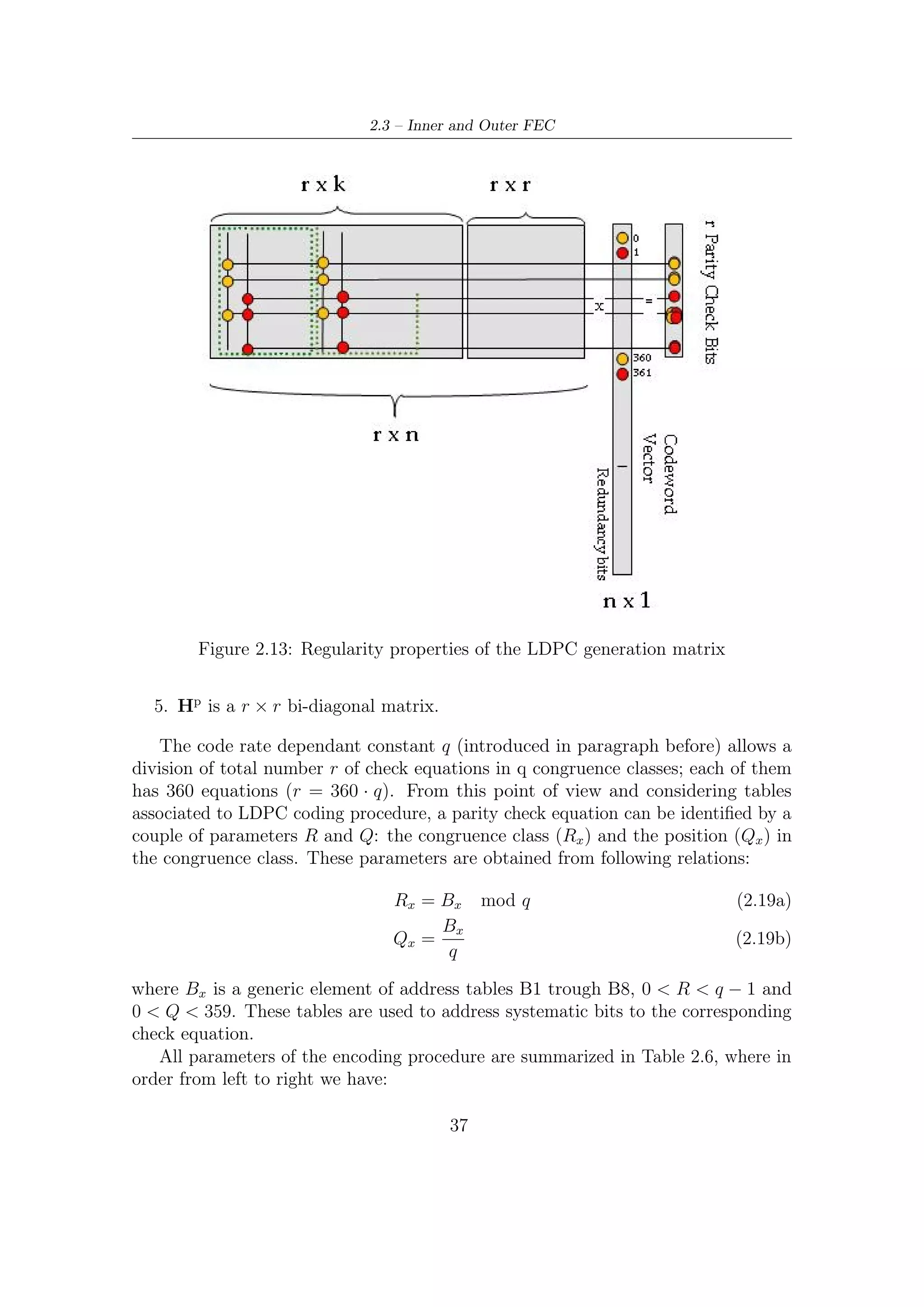
Following considerations can be done:
1. The sparse matrix Hd is constituted by NS sub-matrices (number of rows of
tables B1 through B8) with r-rows and 360-columns, each of which is specified
by a row of the tables B1 through B8; in detail, addresses of ones in the first
column of each matrices is specified by a row of these tables.
2. Each column of the sub-matrices constituting Hd can be obtained via a cyclic
shift of the first column, in which the shift is of a number of positions (rows)
equal to q. The shift is cyclic since it is reduced modulo m, the number of the
rows of each sub-matrix.
3. Hd has a fixed number of ones per row (dc ), depending on coding rate.
4. Number of ones per column in each sub-matrix is not fixed; tables B1 through
B8 in fact has col1 columns in the first row1 rows and col2 columns for row2
(=NS -row1) rows; this means that first row1 sub-matrices of Hd have col1
ones per column, while row2 sub-matrices have col2 ones per column.
36

46. 2.3 – Inner and Outer FEC
Figure 2.13: Regularity properties of the LDPC generation matrix
5. Hp is a r × r bi-diagonal matrix.
The code rate dependant constant q (introduced in paragraph before) allows a
division of total number r of check equations in q congruence classes; each of them
has 360 equations (r = 360 · q). From this point of view and considering tables
associated to LDPC coding procedure, a parity check equation can be identified by a
couple of parameters R and Q: the congruence class (Rx ) and the position (Qx ) in
the congruence class. These parameters are obtained from following relations:
Rx = Bx mod q (2.19a)
Bx
Qx = (2.19b)
q
where Bx is a generic element of address tables B1 trough B8, 0 < R < q − 1 and
0 < Q < 359. These tables are used to address systematic bits to the corresponding
check equation.
All parameters of the encoding procedure are summarized in Table 2.6, where in
order from left to right we have:
37

47. 2 – DVB-S2 MODEM Concepts and Architecture
1. Rate: LDPC coding rate
2. r = n − k: number of code parity bits
3. q = 180 · (1 − R): code rate dependent constant
4. dc : check nodes degree (number of bits per parity check equation)
5. NS = 180 − q = k/360 = row1 + row2: number of sub-matrices r × 360 of
HNS
6. row1: number of sub-matrices with col1 ones per column
7. row2: number of sub-matrices with col2 ones per column
8. col1: variable nodes degree with 0 < index < 360 · row1
9. col2: variable nodes degree with 360 · row1 < index < k
10. #Bx: total number of elements in tables B1 through B8
Rate dc q NS k bit r bit row1 row2 col1 col2 #Bx
1/4 2 135 45 16200 48600 15 30 12 3 270
1/3 3 120 60 21600 43200 20 40 12 3 360
2/5 4 108 72 25920 38880 24 48 12 3 432
1/2 5 90 90 32400 32400 36 54 8 3 450
3/5 9 72 108 38880 25920 36 72 12 3 648
2/3 8 60 120 43200 21600 12 108 13 3 480
3/4 12 45 135 48600 16200 15 120 12 3 540
4/5 16 36 144 51840 12960 18 126 11 3 576
5/6 20 30 150 54000 10800 15 135 13 3 600
8/9 25 20 160 57600 7200 20 140 4 3 500
9/10 28 18 162 58320 6480 18 144 4 3 504
Table 2.6: LDPC parameters for the encoding procedure.
2.4 Modem Performance
Spectral efficiency provided by DVB-S2 ranges from about 0,5 bpsHz−1 , using the
QPSK 1/4, to 4,5 bpsHz−1 , using the 32APSK 9/10; Es /N0 goes from −2,4 dB to
16 dB (AWGN channel and an ideal demodulation have been assumed), as also
38

48. 2.4 – Modem Performance
illustrated in Figure 2.15. This performance has been computed by computer
simulations [1, 7] at a Packet Error Rate (PER) equal to 10−7 , corresponding about
to one erroneous Transport Stream Packet per transmission hour in a 5 Mbit/s video
service On an AWGN channel7 , DVB-S2 gives an increase of transmission capacity
(about 20-35%) compared to DVB-S and DVB-DNSG under the same transmission
conditions.
The DVB-S2 system may be used in ‘single carrier per transponder’ or in ‘multiple-
carriers per transponders’ (FDM). On a transponder with the single carrier con-
figuration, the transmission rate Rs can be adapted to available bandwidth (at
−3 dB) in order to obtain the maximum transmission capacity compatible with the
acceptable signal degradation due to transponder bandwidth limitations. In the
multiple-carrier configuration (Frequency Division Multiplexing), the symbol rate
Rs must be adapted to the BS (Broadcasting Services) frequencies interval so as
to optimize transmissive capacity while keeping the mutual interferences between
adjacent carriers at acceptable level.
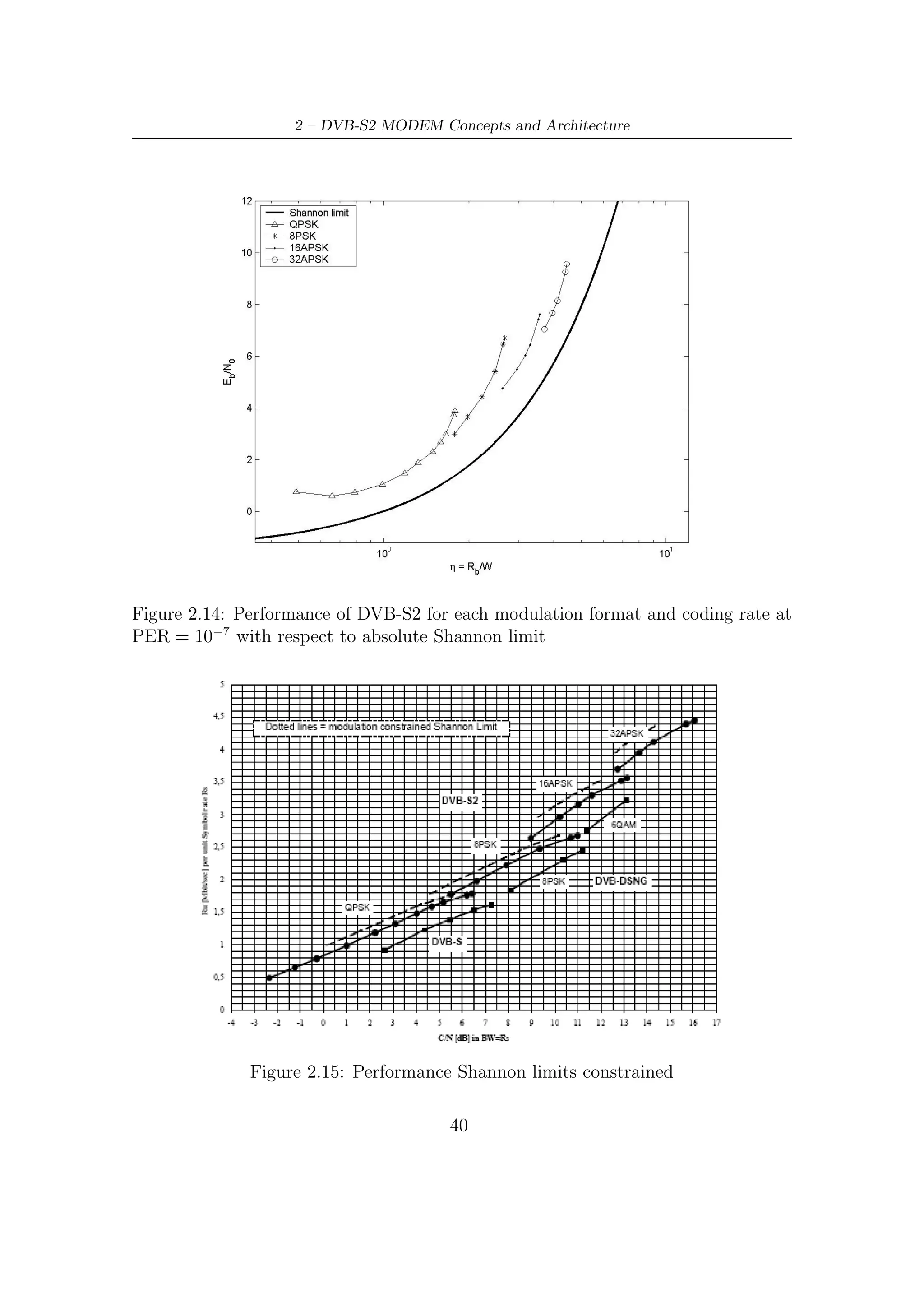
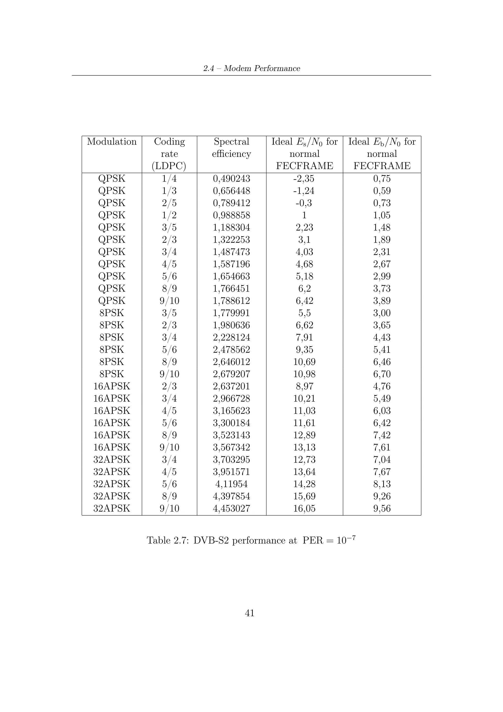
Figure 2.14 shows the performance achieved by the modem architecture with
respect to the unconstrained (from modulation levels and block length of codes)
E
Shannon limit. The ideal Nb ratios in Table 2.7 for each operating mode has been
0
Es
derived from the ideal N0 ratios by using the following dB-relation
Eb Es
= − 10 log10 (ηCM ) (2.20)
N0 N0
where ηCM is the ideal joint efficiency of modulation and coding adopted to transmit
symbols.
Figure 2.15 shows, over the plane C/N – spectral efficiency, the overall perfor-
mance compared to either the constrained Shannon bounds or the DVB-S performance.
The gain of DVB-S2 with respect to DVB-S in terms of C/N , for a given spectral
efficiency, remains virtually constant, around 2 − 2,5 dB [7, 6].
7
We remind that the performance over AWGN channels represents in communications an
upper bound to the performance over more realistic channels. For this reason, comparison of the
performance between two systems can be accomplished without any loss of generality over an
AWGN environment. Comparisons under gaussian hypotheses are expected to be virtually the
same over any non-gaussian environment/channel.
39

49. 2 – DVB-S2 MODEM Concepts and Architecture
Figure 2.14: Performance of DVB-S2 for each modulation format and coding rate at
PER = 10−7 with respect to absolute Shannon limit
Figure 2.15: Performance Shannon limits constrained
40

50. 2.4 – Modem Performance
Modulation Coding Spectral Ideal Es /N0 for Ideal Eb /N0 for
rate efficiency normal normal
(LDPC) FECFRAME FECFRAME
QPSK 1/4 0,490243 -2,35 0,75
QPSK 1/3 0,656448 -1,24 0,59
QPSK 2/5 0,789412 -0,3 0,73
QPSK 1/2 0,988858 1 1,05
QPSK 3/5 1,188304 2,23 1,48
QPSK 2/3 1,322253 3,1 1,89
QPSK 3/4 1,487473 4,03 2,31
QPSK 4/5 1,587196 4,68 2,67
QPSK 5/6 1,654663 5,18 2,99
QPSK 8/9 1,766451 6,2 3,73
QPSK 9/10 1,788612 6,42 3,89
8PSK 3/5 1,779991 5,5 3,00
8PSK 2/3 1,980636 6,62 3,65
8PSK 3/4 2,228124 7,91 4,43
8PSK 5/6 2,478562 9,35 5,41
8PSK 8/9 2,646012 10,69 6,46
8PSK 9/10 2,679207 10,98 6,70
16APSK 2/3 2,637201 8,97 4,76
16APSK 3/4 2,966728 10,21 5,49
16APSK 4/5 3,165623 11,03 6,03
16APSK 5/6 3,300184 11,61 6,42
16APSK 8/9 3,523143 12,89 7,42
16APSK 9/10 3,567342 13,13 7,61
32APSK 3/4 3,703295 12,73 7,04
32APSK 4/5 3,951571 13,64 7,67
32APSK 5/6 4,11954 14,28 8,13
32APSK 8/9 4,397854 15,69 9,26
32APSK 9/10 4,453027 16,05 9,56
Table 2.7: DVB-S2 performance at PER = 10−7
41

51. 2 – DVB-S2 MODEM Concepts and Architecture
42

52. Chapter 3
BCH Encoding Algorithms for
DVB-S2 Digital Transmissions
3.1 Encoding Algorithm Description
As introduced in Section , the systematic encoding of a message
m = (mkBCH −1 , mkBCH −2 , . . . , m1 , m0 ) (3.1)
here expressed in vectorial form, provides a codeword
c = (mkBCH −1 , mkBCH −2 , . . . , m1 , m0 , dnBCH −kBCH −1 , . . . , d0 ) (3.2)
composed of r = nBCH − kBCH redundancy bits, aimed at protecting information
messages, in the least significant positions. Codewords in systematic form have in
the most significant positions the exact replica of information bits.
According to the cyclic code theory (see Appendix B), the systematic encoding
of messages can be carried out through these three steps:
1. Multiplication of the message polynomial m(x) by xr . It can be easily realized
through a left shift of the information bits by r positions and a zero padding
of the least significant r bits.
2. Division of this vector by the polynomial generator. Coefficients of the remain-
der, expressed in polynomial form
d(x) = dr−1 xr−1 + dr−2 xr−2 + . . . + d1 x1 + d0 (3.3)
represent the r parity bits.
43

53. 3 – BCH Encoding Algorithms for DVB-S2 Digital Transmissions
3. Finally, as also stated in Section A.1,
xr m(x) − d(x) (3.4)
provides a codeword. Furthermore, since we are in GF (2) and thus −d(x) =
d(x), the expression (3.4) can be rewritten as
xr m(x) + d(x) (3.5)
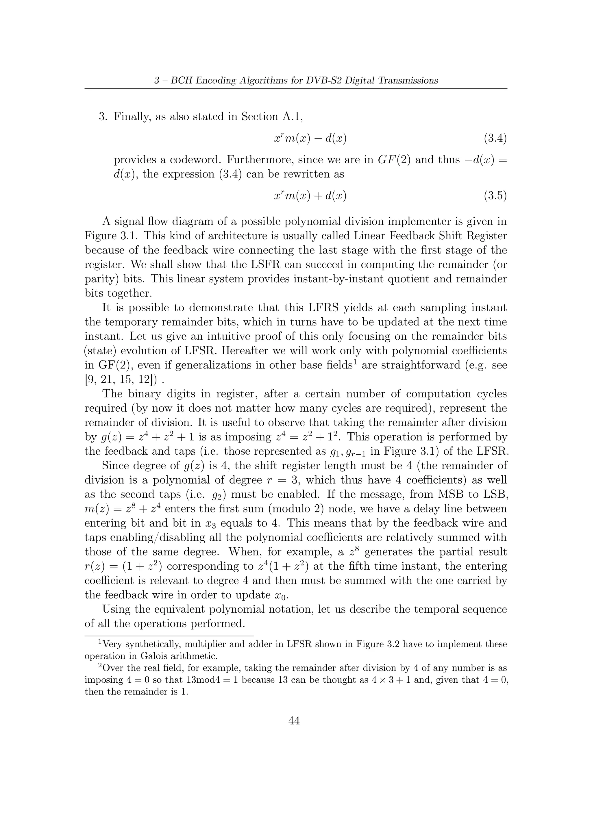
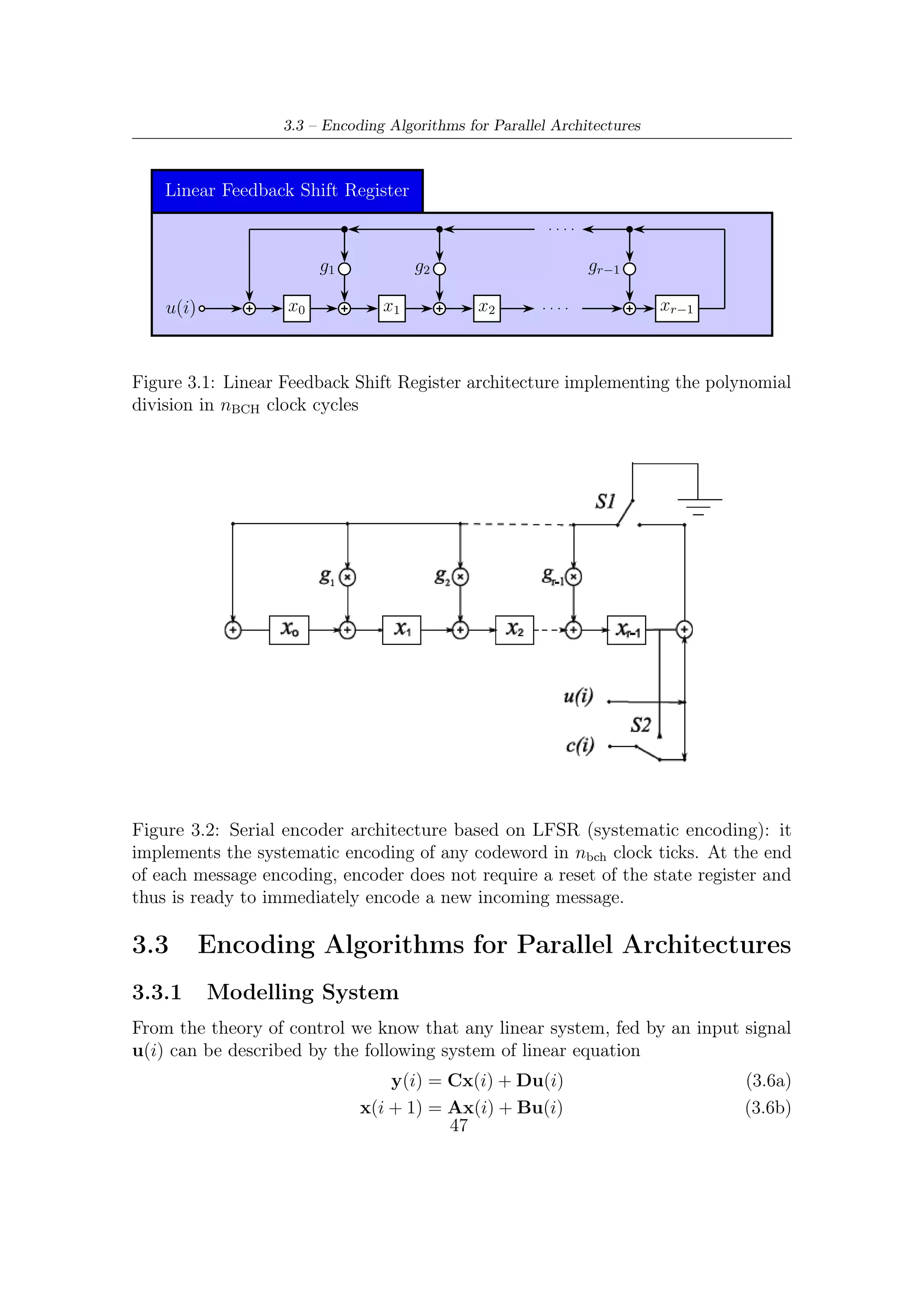
A signal flow diagram of a possible polynomial division implementer is given in
Figure 3.1. This kind of architecture is usually called Linear Feedback Shift Register
because of the feedback wire connecting the last stage with the first stage of the
register. We shall show that the LSFR can succeed in computing the remainder (or
parity) bits. This linear system provides instant-by-instant quotient and remainder
bits together.
It is possible to demonstrate that this LFRS yields at each sampling instant
the temporary remainder bits, which in turns have to be updated at the next time
instant. Let us give an intuitive proof of this only focusing on the remainder bits
(state) evolution of LFSR. Hereafter we will work only with polynomial coefficients
in GF(2), even if generalizations in other base fields1 are straightforward (e.g. see
[9, 21, 15, 12]) .
The binary digits in register, after a certain number of computation cycles
required (by now it does not matter how many cycles are required), represent the
remainder of division. It is useful to observe that taking the remainder after division
by g(z) = z 4 + z 2 + 1 is as imposing z 4 = z 2 + 12 . This operation is performed by
the feedback and taps (i.e. those represented as g1 , gr−1 in Figure 3.1) of the LFSR.
Since degree of g(z) is 4, the shift register length must be 4 (the remainder of
division is a polynomial of degree r = 3, which thus have 4 coefficients) as well
as the second taps (i.e. g2 ) must be enabled. If the message, from MSB to LSB,
m(z) = z 8 + z 4 enters the first sum (modulo 2) node, we have a delay line between
entering bit and bit in x3 equals to 4. This means that by the feedback wire and
taps enabling/disabling all the polynomial coefficients are relatively summed with
those of the same degree. When, for example, a z 8 generates the partial result
r(z) = (1 + z 2 ) corresponding to z 4 (1 + z 2 ) at the fifth time instant, the entering
coefficient is relevant to degree 4 and then must be summed with the one carried by
the feedback wire in order to update x0 .
Using the equivalent polynomial notation, let us describe the temporal sequence
of all the operations performed.
1
Very synthetically, multiplier and adder in LFSR shown in Figure 3.2 have to implement these
operation in Galois arithmetic.
2
Over the real field, for example, taking the remainder after division by 4 of any number is as
imposing 4 = 0 so that 13mod4 = 1 because 13 can be thought as 4 × 3 + 1 and, given that 4 = 0,
then the remainder is 1.
44

54. 3.1 – Encoding Algorithm Description
1. All the register flip flops are set to 0. Coefficient of z 8 enter x0 , so determining
x = (1, 0, 1, 0). We can represent the polynomial division together with digits
in the flip flops by the following expression
(r1 (z) = 1 + 0 · z 1 + 0 · z 2 + 0 · z 3 ) · z 8
where ri (z) represent the partial remainder at i-th iteration.
2.
(r2 (z) = 0 + 1 · z 1 + 0 · z 2 + 0 · z 3 ) · z 7 + (m2 (z) = 0 · z 7 )
3.
(r3 (z) = 0 + 0 · z 1 + 1 · z 2 + 0 · z 3 ) · z 6 + (m3 (z) = 0 · z 6 )
4.
(r4 (z) = 0 + 0 · z 1 + 0 · z 2 + 1 · z 3 ) · z 5 + (m4 (z) = 0 · z 5 )
5. Here we have (r5 (z) = 1 + 0 · z 1 + 1 · z 2 + 0 · z 3 ) · z 4 + (m5 (z) = 1 · z 4 ) and then
(r5 (z) = 0 + 0 · z 1 + 1 · z 2 + 0 · z 3 ) · z 4
6.
(r6 (z) = 0 + 0 · z 1 + 0 · z 2 + 1 · z 3 ) · z 3 + (m6 (z) = 0 · z 3 )
7.
(r7 (z) = 1 + 0 · z 1 + 1 · z 2 + 0 · z 3 ) · z 2 + (m7 (z) = 0 · z 2 )
8.
(r8 (z) = 0 + 1 · z 1 + 0 · z 2 + 1 · z 3 ) · z 1 + (m8 (z) = 0 · z 1 )
9.
(r9 (z) = 1 + 0 · z 1 + 0 · z 2 + 0 · z 3 ) · z 0 + (m9 (z) = 0 · z 0 )
r(z) = r9 (z) corresponding to x = (1, 0, 0, 0) is also the result of division by
g(z).
The key observation to be made in order to understand the encoding process is
interpreting each delay tier as the degree of a polynomial (like z-transform).
For the architecture in Figure 3.2, analogous observations upon delay tier between
input and output can be made. Here the entering coefficients are summed with the
maximum degree coefficients of the partial remainder ri (z) at each clock cycle, and
thus the delay tier is exactly 0. If the result of this sum is 1 then the feedback is
enabled, else it does not. As we shall show in the next section, the choice of feeding
the shift register by the right-hand side allows us to achieve better performance.
45

55. 3 – BCH Encoding Algorithms for DVB-S2 Digital Transmissions
3.2 Serial Architectures
A problem not yet dealt with is how (and when) the parity bits, once computed, can
be extracted from the register. As shown in the previous section, LFSR in Figure 3.1
gives the parity bits as all the bits of message-zero-padded, m(x)xr , enter the fist
sum (modulo 2) node. Therefore, provided that the remainder after division can be
fetched and stored in a single clock tick, this LFSR takes nBCH clock cycles to yield
the wanted result.
It is interesting to notice that only at a certain discrete time instant (they further-
more fall periodically) the registers of LFSR contain redundancy bits representing
the remainder after division. This drawback prevents this type of architecture from
working serially because results of division algorithm have to be properly fetched
and stored in any other register when the parity bits are ready.
As just noticed, architecture in Figure 3.1 is slightly unsuitable for a serial
systematic encoder since results of divisions (redundancy bits) have to be read in
parallel at every (j + 1)nBCH instant for j = 0, 1, 2 . . .. This can be technically
performed, but however the architecture would not be serial anymore. Nevertheless,
these facts will become quite interesting in parallelization of the architecture.
On the other hand, a mere serial hardware architecture is illustrated in Figure 3.2.
Differently from above, here the encoder is fed by the opposite side, thus immediately
enabling the feedback, allowing the structure so devised to yield the remainder at
every (j + 1)kBCH instead of (j + 1)nBCH for j = 0, 1, 2 . . .. This permits to read
serially parity bits and, besides, set (each register is reset) the device so as to make
it ready to encode properly next incoming bit streams. Serial encoding in systematic
form is accomplished (see Figure 3.2) by:
Systematic Bits Transmission and Parity Computation For clock cycles 1
to kBCH , the information bits are transmitted in the natural order (switch S2
in position 2), while also feeding the shift register, to allow parity bits to be
calculated in the Linear Feedback Shift Register (LFSR) (to that purpose,
switch S1 must be on, activating the feedback mode).
Parity Bits Transmission For clock cycles kBCH + 1 to nBCH , the parity bits in
the LFSR are transmitted (switch S2 in position 1) and the LFSR feedback
mode is switched off (by setting S1 off).
From the above timing consideration, it follows that the latter architecture,
spending kBCH clock cycles against nBCH , performs more efficiently encoding in case
of parallel fetching of the parity bits, as we shall see later on.
46

56. 3.3 – Encoding Algorithms for Parallel Architectures
Linear Feedback Shift Register
g1 g2 gr−1
u(i) x0 x1 x2 xr−1
Figure 3.1: Linear Feedback Shift Register architecture implementing the polynomial
division in nBCH clock cycles
Figure 3.2: Serial encoder architecture based on LFSR (systematic encoding): it
implements the systematic encoding of any codeword in nbch clock ticks. At the end
of each message encoding, encoder does not require a reset of the state register and
thus is ready to immediately encode a new incoming message.
3.3 Encoding Algorithms for Parallel Architectures
3.3.1 Modelling System
From the theory of control we know that any linear system, fed by an input signal
u(i) can be described by the following system of linear equation
y(i) = Cx(i) + Du(i) (3.6a)
x(i + 1) = Ax(i) + Bu(i) (3.6b)
47

57. 3 – BCH Encoding Algorithms for DVB-S2 Digital Transmissions
where (3.6a) expresses its outcomes y(i) at each sampling (discrete) instant, while
(3.6b) describes its trajectory of state x(i), i.e., the state evolution of the linear
system in question. Without descending in further details, we shall particularize
both equations for the linear feedback shift register shown in Figure 3.1 and, starting
from them, find equations relevant to an architecture with a p degree of parallelism.
We shall notice that they will perfectly match with system (3.6).
The Linear Feedback Shift Register (LFSR) depicted in Figure 3.1 is a linear
system, and thus can be described by the well known output equation expressing
y(i), the scalar output, and the state transition equation expressing the vector state
x(i) as a function of the discrete time i
y(i) = cx(i) + d · u(i) (3.7a)
x(i + 1) = Ax(i) + bu(i) (3.7b)
In particular, for the desired parallel BCH encoding procedure, we are only
interested in the (state) vector
T
x(i) = x0 (i) x1 (i) . . . . . . xr−1 (i) (3.8)
and in its temporal evolution/transition because x(i) represents the parity bits after
the required number of computation cycles. Thus, hereafter we shall focus only
on (3.7b). The scalar u(i) indicates the input at the sampling instant i, as put in
evidence in Figure 3.1 and Figure 3.2. The matrix A models the state evolution of
the system in absence of external stimulus (i.e., u(i) = 0), and thus is usually called
the state transition matrix. For analogous reasons, the column vector b is called as
the input-to-state transfer relationship.
The form of A, b depends uniquely on the position of taps and connections in the
LFSR. In other words, that form is strongly dependent on the selected architecture
implementing the encoding algorithm. More precisely, the matrix A depends on the
taps collocations of LSFR, whereas vector b depends on where the input/s is/are
connected to the system.
Now, referring to the LFSR architecture depicted in Figure 3.1, which can yield
the redundancy bits after nBCH clock cycles, we can write, on the one hand,
   
0 0 . . . 0 g0 1
 1 0 . . . 0 g1   0 
 .   . 
A =  . 1 . . . 0 g2 
. b= . . (3.9)
   
 .
. ... . . . 
.
  . 
 . 
 . . . .
0 0 . . . 1 gr−1 0
where A, r by r state transition square matrix, contains in the last column the
polynomial generator coefficient except for its coefficient of maximum degree. On
48

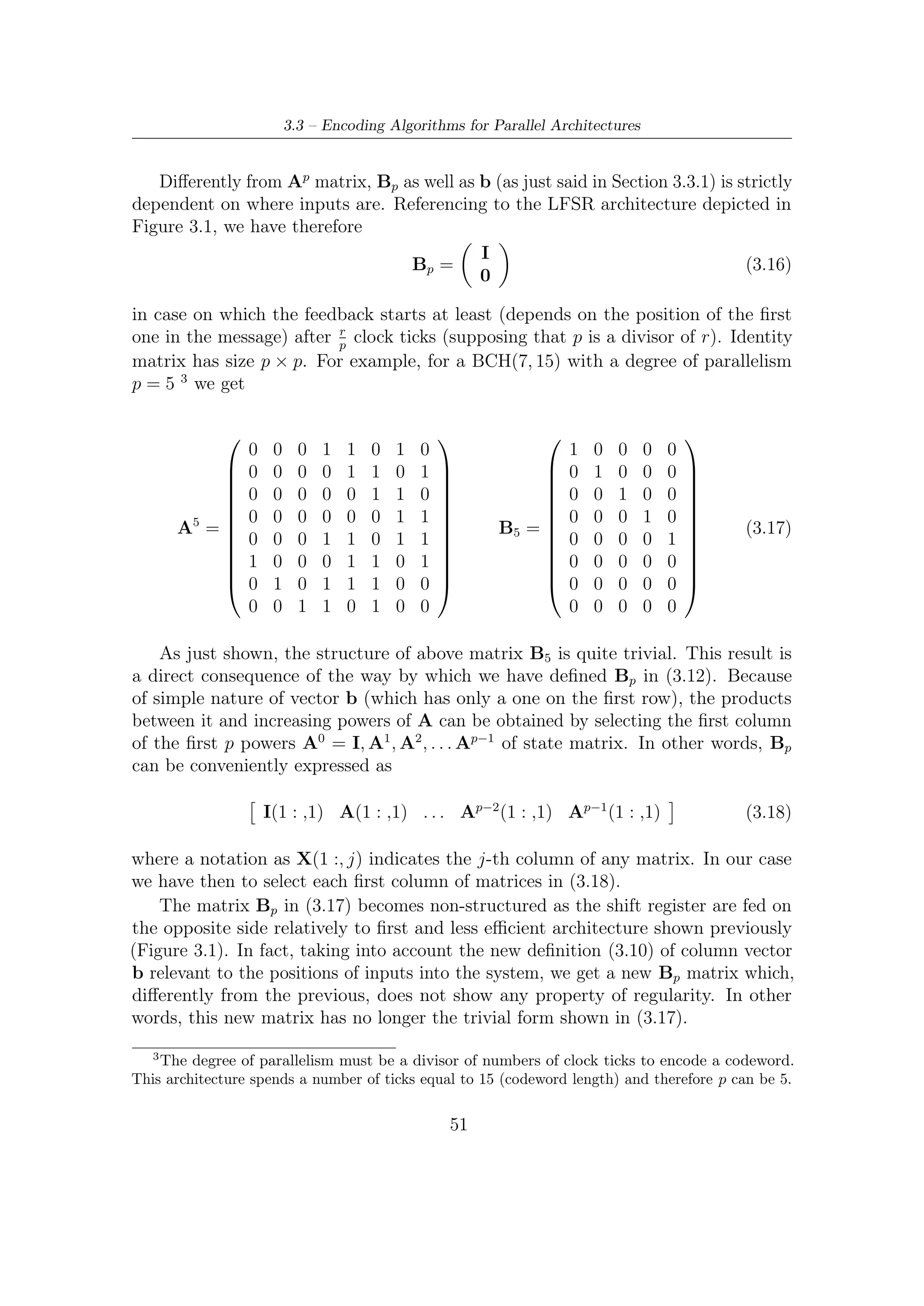
58. 3.3 – Encoding Algorithms for Parallel Architectures
the other hand, column vector b of length r gives a mathematical representation of
the physical input-to-system connections.
As introduced in Section 3.2, the adoption of the architecture in Figure 3.2
permits to save some clock ticks. Not surprisingly, only b has changed its form
whereas the representation of matrix A given in (3.9) still holds. Since inputs enter
now from the right-hand side, we have the new column vector
 
g0
 g1 
 . 
b= .  . (3.10)
 
 . 
 .  .
gr−1
which models – as before – the input incidence on the system state.
3.3.2 Parallel Linear System Description
In the previous section we have briefly described a possible model of system which
can be easily exploited in parallelizing a general serial architecture with a degree of
parallelism p. Starting from (3.7b) and applying instant-by-instant and recursively
the following substitutions
x(i) = Ax(i − 1) + bu(i − 1)
x(i − 1) = Ax(i − 2) + bu(i − 2)
.
.
.
x(i − p + 1) = Ax(i − p) + bu(i − p)
x(i) = A [Ax(i − 2) + bu(i − 2)] + bu(i)
= A2 x(i − 2) + Abu(i − 2) + bu(k − 1)
we can observe that the evolution of this system at a generic sampling instant i
depends on
• the state vector relevant to a generic former instant;
• a set of former inputs whose cardinality is equal to the difference among the
current time index and the former instant selected.
This is equivalent, from an architectural implementation point of view, in feed-
ing the encoding processor by a set of parallel inputs, associating to each of the
multiple input wires a different (multiple) time instant. Hence, parallelization is
straightforwardly achieved.
49

59. 3 – BCH Encoding Algorithms for DVB-S2 Digital Transmissions
Returning to the above expression, the system evolution for a generic degree of
parallelism p is modelled by the following state equation
p−1
x(i) = Ap (i − p) + Ak bu(i − k − 1) (3.11)
k=0
Now, setting the column vectors Ak b as follows
b Ab . . . Ap−2 b Ap−1 b (3.12)
we can define a new r by p Bp matrix which represent the incidence of the last p
inputs
T
u(ip) = u(ip − 1) u(ip − 2) . . . . . . u [p(i − 1))] (3.13)
on the system evolution. Considering both (3.12) and (3.13), we can therefore rewrite
the state equation (3.11) as
x(ip) = Ap x [(i − 1)p] + Bp u(ip) (3.14)
p−1
where the sum k=0 Ak bu(i − k − 1) has just been replaced by the above matrices
product.
3.3.3 Matrices Structure and Properties
In every practical case, the wanted degree of parallelism is strictly less than the
number of registers containing the remainder bits at the end of every bit stream
processing. For this reason, in this section we shall describe the main characteristics
of matrices Ap and Bp only within the range 0 < p ≤ r of our interest.
Therefore for a generic degree p (within the above specified range) we have
0 C1
Ap = (3.15)
I C2
where
• 0 represents a null p × p matrix;
• I represent a square r − p by r − p identity matrix;
• C1 is a p × p matrix where each row represents the combinatorial connections
(1 when it is active, 0 otherwise) between last and first p bits of vector x(i);
• C2 is a (r − p) × p matrix where each row represents the combinatorial connec-
tions between last p bits and the remaining bits of the vector x(i)
50

60. 3.3 – Encoding Algorithms for Parallel Architectures
Differently from Ap matrix, Bp as well as b (as just said in Section 3.3.1) is strictly
dependent on where inputs are. Referencing to the LFSR architecture depicted in
Figure 3.1, we have therefore
I
Bp = (3.16)
0
in case on which the feedback starts at least (depends on the position of the first
r
one in the message) after p clock ticks (supposing that p is a divisor of r). Identity
matrix has size p × p. For example, for a BCH(7, 15) with a degree of parallelism
p = 5 3 we get
   
0 0 0 1 1 0 1 0 1 0 0 0 0

 0 0 0 0 1 1 0 1 


 0 1 0 0 0 


 0 0 0 0 0 1 1 0 


 0 0 1 0 0 

5
 0 0 0 0 0 0 1 1   0 0 0 1 0 
A =  B5 =   (3.17)

 0 0 0 1 1 0 1 1 


 0 0 0 0 1 


 1 0 0 0 1 1 0 1 


 0 0 0 0 0 

 0 1 0 1 1 1 0 0   0 0 0 0 0 
0 0 1 1 0 1 0 0 0 0 0 0 0
As just shown, the structure of above matrix B5 is quite trivial. This result is
a direct consequence of the way by which we have defined Bp in (3.12). Because
of simple nature of vector b (which has only a one on the first row), the products
between it and increasing powers of A can be obtained by selecting the first column
of the first p powers A0 = I, A1 , A2 , . . . Ap−1 of state matrix. In other words, Bp
can be conveniently expressed as
I(1 : ,1) A(1 : ,1) . . . Ap−2 (1 : ,1) Ap−1 (1 : ,1) (3.18)
where a notation as X(1 :, j) indicates the j-th column of any matrix. In our case
we have then to select each first column of matrices in (3.18).
The matrix Bp in (3.17) becomes non-structured as the shift register are fed on
the opposite side relatively to first and less efficient architecture shown previously
(Figure 3.1). In fact, taking into account the new definition (3.10) of column vector
b relevant to the positions of inputs into the system, we get a new Bp matrix which,
differently from the previous, does not show any property of regularity. In other
words, this new matrix has no longer the trivial form shown in (3.17).
3
The degree of parallelism must be a divisor of numbers of clock ticks to encode a codeword.
This architecture spends a number of ticks equal to 15 (codeword length) and therefore p can be 5.
51

61. 3 – BCH Encoding Algorithms for DVB-S2 Digital Transmissions
3.4 Some Considerations
From a hardware point of view, following considerations can be made:
1. since codeword length compliant with DVB-S2 standard is long (either short
or long FECFRAME), a serial encoder (e.g., that depicted in Figure 3.2) may
be rather inefficient and slow;
2. parallel architectures are more flexible solutions when different t-error correction
BCH codes are needed. Since the standard provides different t (for BCH) that
can be switched on a frame basis, encoder is required to be versatile;
3. the overall architecture (inner LDPC encoder in parallel implementation) has
to be taken into account and a parallel encoder make the interface design
simpler.
On the contrary, serial architectures, being based on an elementary LSFR sub-
structure, are rather simpler than their parallel version. But, for the reasons
enumerated above, they have not been taken in consideration to design the encoding
section of DVB-S2.
52

62. Chapter 4
Hardware Implementation of BCH
Encoder
4.1 FEC Encoding Section
The parallelism of the input memory of the LDPC encoding section suggests a p = 8
degree of parallelism for BCH architecture. First, because LDPC input memory
requires 360 bits and LDPC encoder processes the same number of bits at every
clock ticks (i.e., it has 360 as degree of parallelism). Hence, p should be a divisor of
360. Second, p should be even a divisor of each BCH block length (nbch ) associated
to LDPC coding rates, provided by DVB-S2. Furthermore, BCH serial architectures
based on LFSRs are, of course, simple to implement, but generally they are very
slow (i.e., they reach typically a lower throughput). Therefore, in order to best
match BCH encoding speed with the frequency requirements imposed by the overall
designed TX DVB-S2 section, we have chosen a degree of parallelism equal to 8.
Encoded bits, passing through an interface circuit, enter LDPC input memory
on a byte basis. The interface allows each codeword coming from BCH encoder to
be read in the proper order and format (recall that a systematic code is required as
output). A block diagram of the overall FEC section is depicted in Figure 4.1.
As we shall detail in the next section, the interface between BCH and LDPC is
constituted by a simple 8 bits multiplexer together with a suited circuitry to store
and download the parity bits after each computation cycle. This interface addresses
properly encoded bits into LDPC input memory and it must be driven by a control
logic based on clock cycles required (see Table 4.1) to provide a codeword.
Another important question to raise up is certainly giving the architecture a
flexible structure so as to succeed in dealing with each coding rate provided by
DVB-S2 FEC. A more versatility, as we shall see, requires an additional usage of
memory: as a matter of fact, some additional coefficient of matrices mentioned in
53

63. 4 – Hardware Implementation of BCH Encoder
Figure 4.1: Block diagram of the overall FEC tx section
the previous chapter must be stored into some LUTs (Look Up Tables).
BCH BCH Coded Ticks to Parity bits Total clock
Uncoded Block NBCH transmit download cycles
Block informative
bits
16008 16200 2001 24 2025
21408 21600 2676 24 2700
25728 25920 3216 24 3240
32208 32400 4026 24 4050
38688 38880 4836 24 4860
43040 43200 5380 20 5400
48408 48600 6051 24 6075
51648 51840 6456 24 6480
53840 54000 6730 20 6750
57472 57600 7184 16 7200
58192 58320 7274 16 7290
Table 4.1: Clock cycles required to provide each codeword for each operating mode
of DVB-S2
54

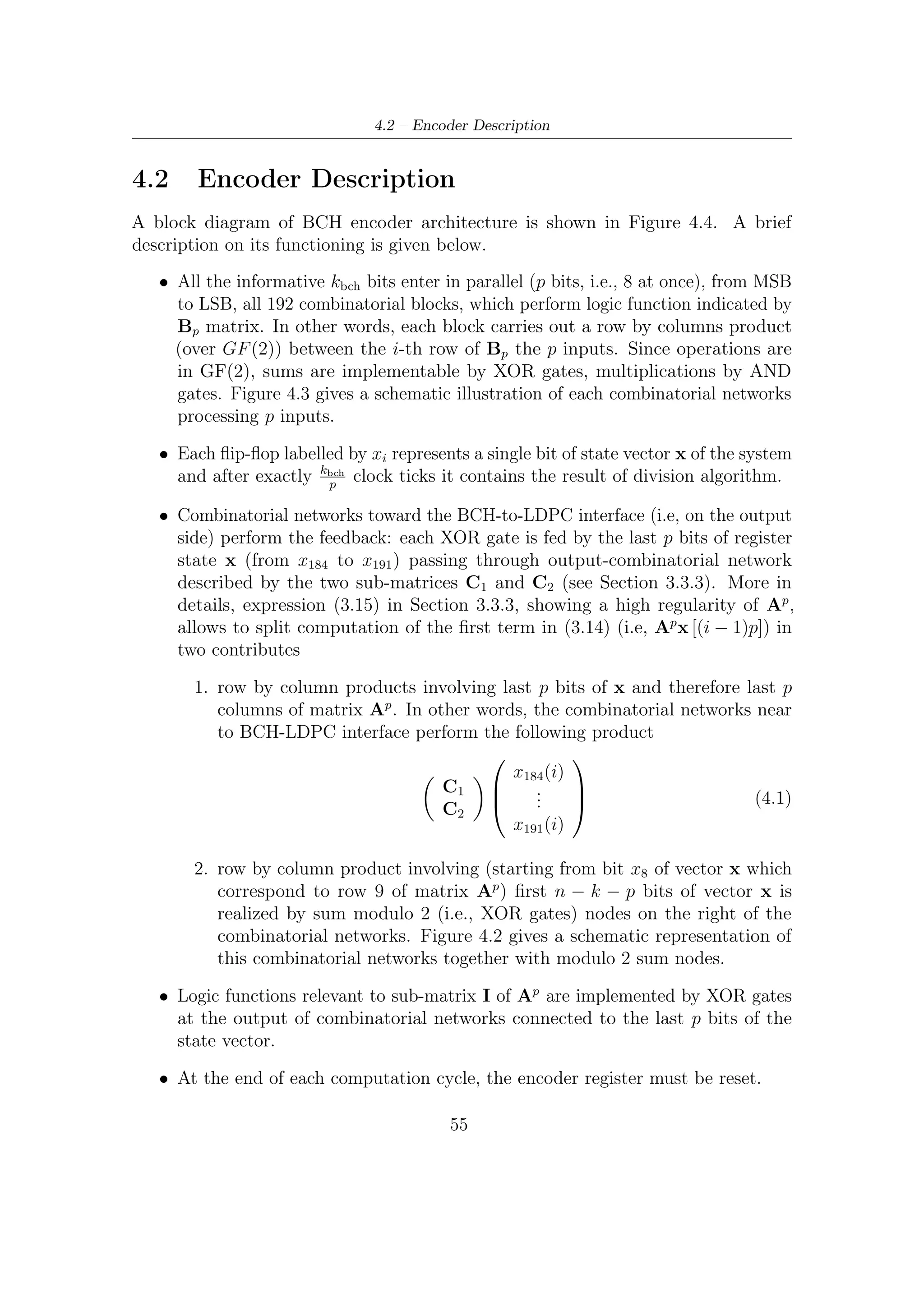
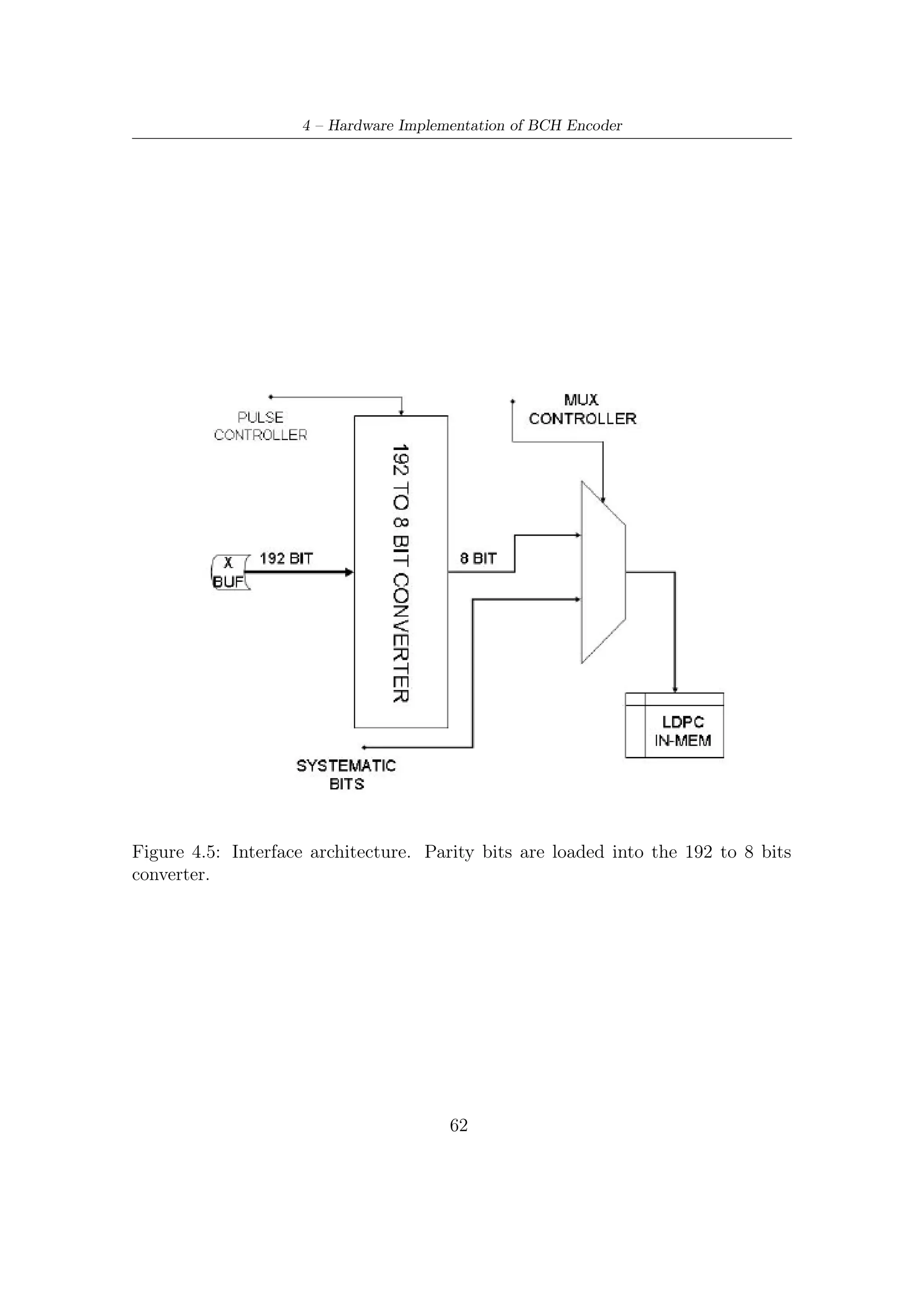
64. 4.2 – Encoder Description
4.2 Encoder Description
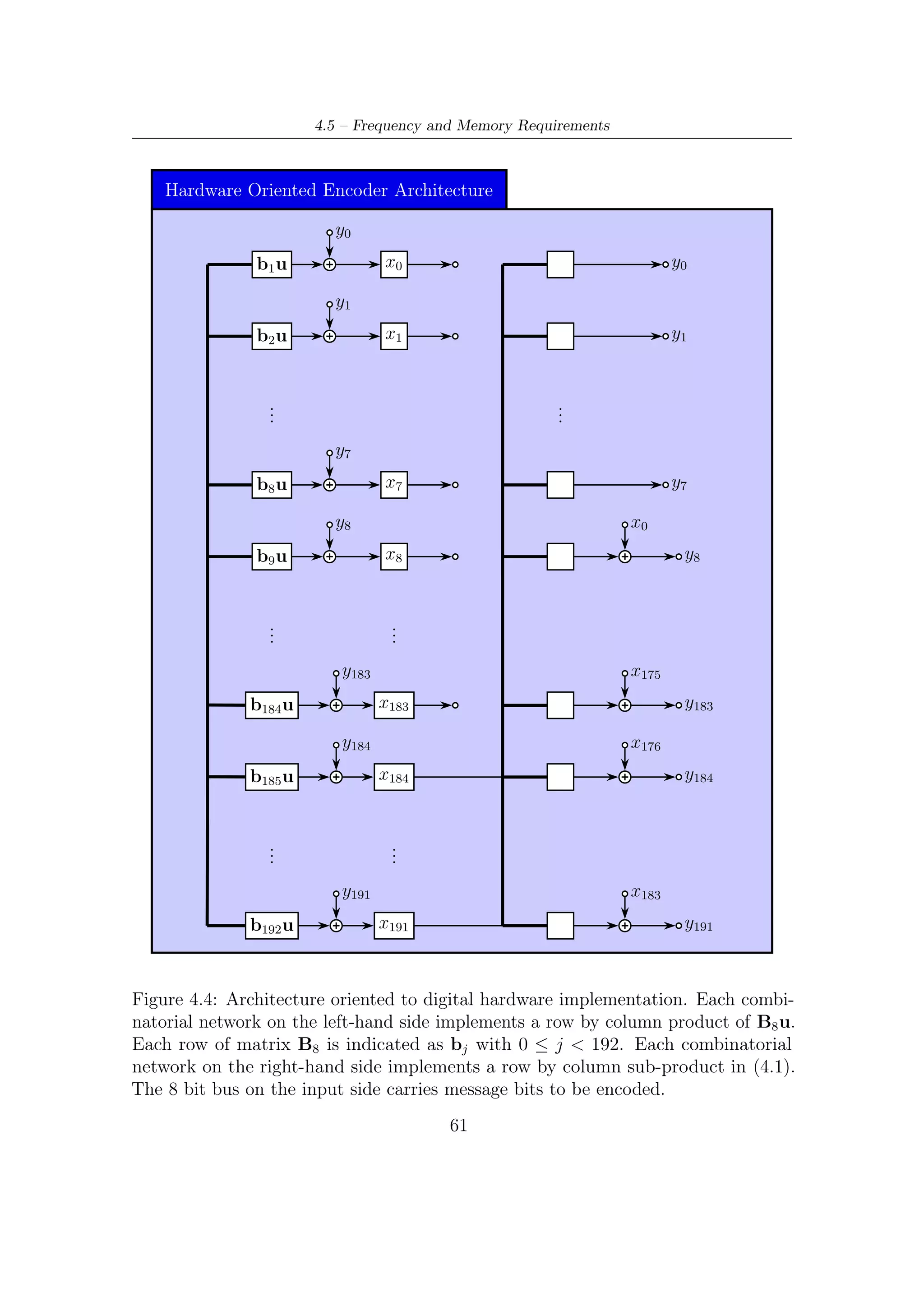
A block diagram of BCH encoder architecture is shown in Figure 4.4. A brief
description on its functioning is given below.
• All the informative kbch bits enter in parallel (p bits, i.e., 8 at once), from MSB
to LSB, all 192 combinatorial blocks, which perform logic function indicated by
Bp matrix. In other words, each block carries out a row by columns product
(over GF (2)) between the i-th row of Bp the p inputs. Since operations are
in GF(2), sums are implementable by XOR gates, multiplications by AND
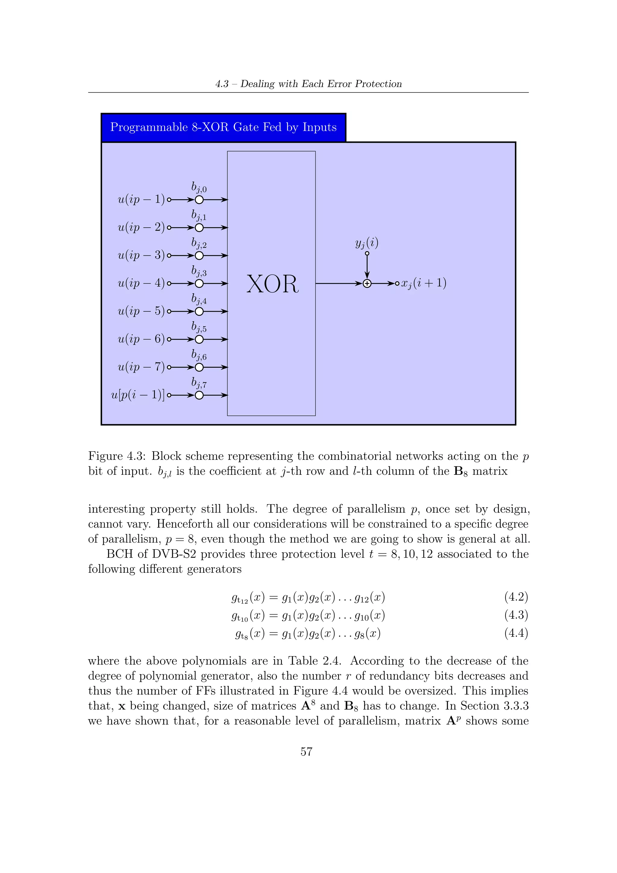
gates. Figure 4.3 gives a schematic illustration of each combinatorial networks
processing p inputs.
• Each flip-flop labelled by xi represents a single bit of state vector x of the system
and after exactly kbch clock ticks it contains the result of division algorithm.
p
• Combinatorial networks toward the BCH-to-LDPC interface (i.e, on the output
side) perform the feedback: each XOR gate is fed by the last p bits of register
state x (from x184 to x191 ) passing through output-combinatorial network
described by the two sub-matrices C1 and C2 (see Section 3.3.3). More in
details, expression (3.15) in Section 3.3.3, showing a high regularity of Ap ,
allows to split computation of the first term in (3.14) (i.e, Ap x [(i − 1)p]) in
two contributes
1. row by column products involving last p bits of x and therefore last p
columns of matrix Ap . In other words, the combinatorial networks near
to BCH-LDPC interface perform the following product
 
x184 (i)
C1  .
. (4.1)

C2
 . 
x191 (i)
2. row by column product involving (starting from bit x8 of vector x which
correspond to row 9 of matrix Ap ) first n − k − p bits of vector x is
realized by sum modulo 2 (i.e., XOR gates) nodes on the right of the
combinatorial networks. Figure 4.2 gives a schematic representation of
this combinatorial networks together with modulo 2 sum nodes.
• Logic functions relevant to sub-matrix I of Ap are implemented by XOR gates
at the output of combinatorial networks connected to the last p bits of the
state vector.
• At the end of each computation cycle, the encoder register must be reset.
55

65. 4 – Hardware Implementation of BCH Encoder
Due to intrinsic simplicity of matrices Ap and Bp (they are only composed by
zeroes and ones), the two combinatorial networks can be implemented in a very
simple way by programmable XOR gates with eight inputs. More in detail, each
coefficient of the above two matrices says which wires have to be connected to each
combinatorial network (XOR).
Programmable 8-XOR Gate Fed by A Portion of State
aj,184
x184
aj,185
x185
aj,186 xj−8 (i) for j ≥ 8
x186
aj,187
x187
aj,188
XOR yj (i)
x188
aj,189
x189
aj,190
x190
aj,191
x191
Figure 4.2: Block scheme of the combinatorial networks acting on the last p bits of
x. aj,l is the coefficient at j-th row and l-th column of A8 matrix
4.3 Dealing with Each Error Protection
Architecture we have shown as far can only address the greater t error protection
modalities. However, DVB-S2 has been designed to operate in ACM (Adaptive
Coding and Modulation) mode, so that a flexible architecture, capable of changing
his behavior on a frame basis, would be more desirable.
From our analysis of the two matrices, we have reach the conclusion that they
are very regular and, even changing the polynomial generator of the code, this
56

66. 4.3 – Dealing with Each Error Protection
Programmable 8-XOR Gate Fed by Inputs
bj,0
u(ip − 1)
bj,1
u(ip − 2)
bj,2 yj (i)
u(ip − 3)
bj,3
u(ip − 4)
bj,4
XOR xj (i + 1)
u(ip − 5)
bj,5
u(ip − 6)
bj,6
u(ip − 7)
bj,7
u[p(i − 1)]
Figure 4.3: Block scheme representing the combinatorial networks acting on the p
bit of input. bj,l is the coefficient at j-th row and l-th column of the B8 matrix
interesting property still holds. The degree of parallelism p, once set by design,
cannot vary. Henceforth all our considerations will be constrained to a specific degree
of parallelism, p = 8, even though the method we are going to show is general at all.
BCH of DVB-S2 provides three protection level t = 8, 10, 12 associated to the
following different generators
gt12 (x) = g1 (x)g2 (x) . . . g12 (x) (4.2)
gt10 (x) = g1 (x)g2 (x) . . . g10 (x) (4.3)
gt8 (x) = g1 (x)g2 (x) . . . g8 (x) (4.4)
where the above polynomials are in Table 2.4. According to the decrease of the
degree of polynomial generator, also the number r of redundancy bits decreases and
thus the number of FFs illustrated in Figure 4.4 would be oversized. This implies
that, x being changed, size of matrices A8 and B8 has to change. In Section 3.3.3
we have shown that, for a reasonable level of parallelism, matrix Ap shows some
57

67. 4 – Hardware Implementation of BCH Encoder
regularity. In practice, its structure shown in (3.15) does not change from t8 to t12 ,
although its coefficients are, of course, subject to variations. Same consideration can
be made upon Bp matrix, which however shows no regularity property for this kind
of architecture.
Figure 4.3 and Figure 4.2 clearly show that these kind of combinatorial network
are programmable by means of their coefficients, determining which wire has to be
connected to the 8-inputs XOR gate and which not. Imposing, for example, that all
of these coefficients are forced to zero, we would get the result of having inhibited
the j-th combinatorial network. This is exactly what we can do to deal with all the
protection level t.
In particular, either A8 or B8 can be embedded into the their largest matrices of
size, respectively, 192 × 192 and 192 × 8 in this way:
Medium Protection Level (t = 10) Matrices (A8 )o and (B8 )o oversized (they
should be 160 × 160 and 160 × 8 respectively) turn out to be as follows
0 0 0
(A8 )o = (B8 )o = (4.5)
0 (A8 )t10 (B8 )t10
This corresponds to inhibit the first 32 couples of combinatorial networks since
their coefficients are all nulls. Thus, all the first 32 FFs (from x0 to x31 ) of the
BCH encoder will contain always zeroes.
Low Protection Level (t = 8) The oversized matrices are build in the same
manner and now the first 64 couples of combinatorial networks are inhibited
since their coefficients are all nulls.
4.4 Interface and Parity Bits Extraction
The interface between BCH and LDPC encoder can be implemented as illustrated in
Figure 4.5. The parity bits, once computed (at nbch clock tick), can be saved (in a
single clock cycle) in a shift register architecture, which has been called in Figure 4.5
192 (or rather, up to 192) to 8 bit converter. In fact, its task is formatting data in
the DVB-S2 format. Furthermore, this kind of architecture allows to write all the
parity bits extracted from BCH encoder (in a single clock tick) into LDPC input
memory with a degree of parallelism equal to 81 .
Further detailing, the converter is composed by 8 shift register blocks with size
equal to 24 bits. In a preliminary fase all the parity bits computed by the BCH
1
Note also that p = 8 is not only a divisor for 360, but also for 192(t = 12), 160(t = 10) and
128(t = 8)
58

68. 4.5 – Frequency and Memory Requirements
encoder are stored in these blocks following the labelling indicated in Figure 4.6 (to
succeed in storing these bits, MUXs between each flip flop can be used). Afterward,
the converter works as a shift register, thus allowing to download data eight at once,
i.e., with a degree of parallelism equal to 8.
To summarize, let us see, in order for each iteration, the operations carried out
by this specific interface:
1. Once the parity bits have been computed, they are stored in another shift
register according to the bit-to-bit mapping illustrated in Figure 4.6. MUXs
between a FF and its neighbor allow to store bits all at once (in parallel) as
they are switched on wires carrying results of encoding (these wires may be
directly connected to the BCH encoder register).
2. As MUXs are switched on wires interconnecting FFs each other, all the bits
previously stored, shifting along FFs, are carried by some ’strategic’ wires
on the 8 bits bus, which conveys parity bits toward the output multiplexer.
Practically, the register is working as a shift register.
3. The output multiplexer has two inputs buses connected to: informative bits
and redundancy bits. MUX should be driven by a proper control logic on the
operating mode basis.
4.5 Frequency and Memory Requirements
Taking into account LDPC outer encoder frequency requirements and imposing a
data rate equal to 1 Gbps, in the worst case, that is, when t = 8 and LDPC code rate
is equal to 9/10, we obtain the maximum frequency requirement so as to guarantee
this challenging performance:
f rame
(fclk )MAX = · 7290 = 125 MHz (4.6)
s
Concerning to memory requirement either, the architecture proposed takes six (two
per each level of BCH protection parameter t) LUTs to store coefficients used by the
combinatorial networks. As a matter of fact, storing of the C1 and C2 sub-matrices
(recall that they represent two sub-blocks, whose aggregated size is 192 × 8, of the A8
matrix) coefficients as well matrix B8 , whose size is 192 × 8, coefficients is required.
To provide an encoder capable of dealing with each t-error protection level, those
matrices have to be saved in LUTs for each t. The size of each LUT is equal to
192 Bytes and thus the BCH encoder, apart from additional memory required by the
59

69. 4 – Hardware Implementation of BCH Encoder
BCH-LDPC interface and the encoder state register, requires an amount of memory
equal to
2 · 3 · 192 B = 1,125 KiB. (4.7)
60

70. 4.5 – Frequency and Memory Requirements
Hardware Oriented Encoder Architecture
y0
b1 u x0 y0
y1
b2 u x1 y1
.
. .
.
. .
y7
b8 u x7 y7
y8 x0
b9 u x8 y8
.
. .
.
. .
y183 x175
b184 u x183 y183
y184 x176
b185 u x184 y184
.
. .
.
. .
y191 x183
b192 u x191 y191
Figure 4.4: Architecture oriented to digital hardware implementation. Each combi-
natorial network on the left-hand side implements a row by column product of B8 u.
Each row of matrix B8 is indicated as bj with 0 ≤ j < 192. Each combinatorial
network on the right-hand side implements a row by column sub-product in (4.1).
The 8 bit bus on the input side carries message bits to be encoded.
61

71. 4 – Hardware Implementation of BCH Encoder
Figure 4.5: Interface architecture. Parity bits are loaded into the 192 to 8 bits
converter.
62

72. 4.5 – Frequency and Memory Requirements
Figure 4.6: 192 to 8 bits converter architecture. Values into each FF represent the
index mapping between the BCH encoder register and the interface register, used to
extract and format data.
63

73. 4 – Hardware Implementation of BCH Encoder
64

74. Chapter 5
Software Package for VHDL
Validation
5.1 Software Implementation of Serial Encoder
This section describes the software implementations of the architecture illustrated
in Figure 3.2. Recall that only this architecture is actually serial since the other
one (depicted in Figure 3.1), which computes parity bits in nbch clock ticks, needs a
parallel fetching of the encoding result and a reset of the register at the end of each
computation cycle1 .
The software implementation shown below simulates the serial architecture de-
picted in Figure 3.2. For the first k clock ticks, the informative bits exits while the
feedback loop is enabled. From k to n instead, the feedback loop is disabled and then
all the parity bits ready to be fetched are carried (serially) to the output while zeros
are going to be stored into each stage of the shift register, thus resetting the register.
This is certainly an advantage with respect to architecture depicted in Figure 3.1,
which requires a parallel fetching of the parity bits together with, in turn, a reset of
the shift register.
To simulate the two different behaviors of the serial encoder, which for k clock
cycles yields the bits of message while for the next one produces the parity bits, a
integer encStep counter has been employed. It follows a useful description of the
used variable:
• ticks is a function parameter and refers to the numbers of iteration/clock-ticks
which have to be simulated; m[], out[], other ones function parameters, are
vector relevant to input and output. The function Run reads from m[] and
write in turn the result of ticks computation cycles.
1
Clearly, in software, this distinction is not so strict
65

75. 5 – Software Package for VHDL Validation
• Vector of integer state[] represent the values contained in each register of the
encoder.
• g[] represent in vectorial form polynomial generator of the BCH code.
• r is the length of the shift register.
void BCHenc : : Run ( i n t t i c k s , i n t ∗m, i n t ∗ o u t )
{
int i , s , j , k ;
i f ( e n c S t e p == n ) { e n c S t e p = 0 ; }
i f ( encStep < k ){
f o r ( i = 0 ; i < t i c k s ; i ++, e n c S t e p ++){
// I f c o n d i t i o n i s t r u e e n a b l e f e e d b a c k
i f ( s t a t e [ r −1]^m[ i ] ) {
f o r ( j = r −1; j >=1; j −−)
s t a t e [ j ] = s t a t e [ j −1]^ g [ j ] ;
state [ 0 ] = 1;
}
else {
// S h i f t i n g o f b i t s
f o r ( j = r −1; j >= 1 ; j −−)
s t a t e [ j ] = s t a t e [ j −1];
state [ 0 ] = 0;
}
o u t [ i ] = m[ i ] ;
}
}
e l s e i f ( e n c S t e p >=k && e n c S t e p < n ) {
f o r ( i = 0 ; i < t i c k s ; i ++, e n c S t e p ++){
out [ i ] = s t a t e [ r −1];
f o r ( j = r −1; j >= 1 ; j −−)
s t a t e [ j ] = s t a t e [ j −1];
state [ 0 ] = 0;
}
}
}
This piece of software works serially, but the user may define the number of iterations
that emulator machine has to perform. Anyway this software emulator, as its more
physical version, takes n clock ticks to encode a single codeword.
5.2 Software Implementations of Parallel Encoder
Matrices A8 and B8 defined in Section 3.3.3 have been pre-computed via software
by a Matlab routine. Useful coefficients of these matrices can be stored in local
variables (software) or in LUT (hardware). Note that, concerning the A8 matrix,
the sub-matrices C1 and C2 should be stored in a dedicated memory for each t-error
correction level to make the architecture flexible.
The first software implementation refers to the slower parallel architecture which
spends n clock ticks to provide codewords associated to messages. Pre-computed
parts of the matrix A8 relevant to each operating modes are loaded and saved in
memory on (n, k) (only those provided by the standard) basis. Matrix Bp , already
defined in (3.16) (see also the example in Section 3.3.3), is trivial and its save in
memory can be avoided since that form corresponds to connect the eight inputs
to the first XOR stage of the architecture. In other words, the 192 combinatorial
66

76. 5.2 – Software Implementations of Parallel Encoder
networks on the input side (depicted in Figure 4.4) in this kind of architecture are
not necessary. The following function is dedicated to simulate the functioning of
combinatorial networks on the output side:
• Feedback combinatorial network acting on the last eight values of the state
register. Function combn(index, n, regold) implements the product row by
column between C1 , C2 and x184 , . . . , x191 .
i n t comb_n ( i n t i n d e x , i n t r , int ∗ reg_old )
{
i n t out , f ;
o u t =0;
f o r ( f =0; f <P ; f ++)
{
o u t=o u t ^(Ap_n [ i n d e x ] [ r−f −1] & r e g _ o l d [ r−f − 1 ] ) ;
}
return ( o u t ) ;
}
The first part of function BCHnclkpar(int n,int k) is relevant to the error
protection level and consequently due to the state vector allocation (recall that
register length can be 128, 160, 192 with respect to t = 8, 10, 12 possible values). In
case of mismatch with the couples n, k, provided by the standard DVB-S2 for the
normal FECFRAME, simulation is aborted. The for cycle in the middle part of
the program updates cyclically the register of the encoder, using the above function
implementing each combinatorial networks. Eventually, output is formatted in the
systematic form complyant with the DVB-S2 standard requirements.
void BCHnclk_par ( i n t n , i n t k )
{
int c l o c k _ t i c k s ;
int ∗ reg , ∗ reg_old ;
int input [P ] ; // p a r a l l e l input bits
/∗ Mode S e l e c t i o n ( t−e r r o r−c o r r e c t i o n ) ∗/
switch ( n−k ) {
case 1 9 2 :
r e g = ( i n t ∗ ) c a l l o c ( n−k , s i z e o f ( i n t ) ) ;
r e g _ o l d = ( i n t ∗ ) c a l l o c ( n−k , s i z e o f ( i n t ) ) ;
break ;
case 1 6 0 :
r e g = ( i n t ∗ ) c a l l o c ( n−k , s i z e o f ( i n t ) ) ;
r e g _ o l d = ( i n t ∗ ) c a l l o c ( n−k , s i z e o f ( i n t ) ) ;
break ;
case 1 2 8 :
r e g = ( i n t ∗ ) c a l l o c ( n−k , s i z e o f ( i n t ) ) ;
r e g _ o l d = ( i n t ∗ ) c a l l o c ( n−k , s i z e o f ( i n t ) ) ;
break ;
default :
f p r i n t f ( s t d o u t , " E r r o r : s i m u l a t i o n a b o r t e d ! n" ) ;
f p r i n t f ( s t d o u t , " P l e a s e i n s e r t a n−k c o u p l e
p r o v i d e d by DVB −S2 FECn" ) ;
exit (0);
}
/∗ Computation o f c l o c k t i c k s r e q u i r e d
t o compute t h e remainder a f t e r d i v i s i o n ∗/
c l o c k _ t i c k s = n/P ;
67

77. 5 – Software Package for VHDL Validation
/∗ Computing remainder ∗/
i n t z =0;
f o r ( i n t i =0; i <c l o c k _ t i c k s ; i ++)
{
/∗ r e f r e s h o f s t a t e ∗/
f o r ( i n t m=0; m <n−k ; m++)
r e g _ o l d [m]= r e g [m ] ;
// /////////////////////////////////////
/////// l o a d i n g o f p a r a l l e l i n p u t //////
f o r ( i n t c o u n t=P−1; count >=0; count −−)
{
z++;
i n p u t [ c o u n t ] = m e s s a g e [ n−z ] ;
}
// /////////////////////////////////////////
/// Computing o f n e x t v a l u e s o f s t a t e /////
i f ( c l o c k _ t i c k s >0)
{
f o r (m=0; m <n−k ; m++)
{
i f (m<P)
r e g [m] = i n p u t [m] ^ comb_n (m, n−k , r e g _ o l d ) ;
else
r e g [m] = comb_n (m, n−k , r e g _ o l d )^ r e g _ o l d [ m−P ] ;
}
}
// ///////////////////////////////////////////
}
/∗ Codeword i n s y s t e m a t i c form ∗/
f o r ( i=n −1; i >n−k −1; i −−)
codeword [ i ] = m e s s a g e [ i ] ;
f o r ( i=n−k −1; i >=0; i −−)
codeword [ i ] = reg [ i ] ;
}
The second implementation is connected to the faster architecture (its correspon-
dent serial version is depicted in Figure 3.2) which spends k clock ticks to compute
parity bits, saving, compared to the first, r clock cycles for each computation cycle or,
i.e., for each encoding cycle. The function combn(index, n, regold) implementing
the combinatorial networks on the output side is the same of the slower architecture
according to what we said in Chapter 3 (i.e. matrix A8 cannot change). Therefore
here we have two functions:
• Function combc(index, input) provides the result of row by column product
between matrix B8 and the inputs.
• Function combn(index, n, regold) implements the product row by column
between C1 , C2 and x184 , . . . , x191 .
i n t comb_c ( i n t i n d e x , int ∗ input )
{
i n t out , f , i n d ;
o u t =0;
i n d=P−1;
f o r ( f =0; f <P ; f ++)
{
68

78. 5.2 – Software Implementations of Parallel Encoder
o u t= o u t ^ ( (C [ i n d e x ] [ f ] ) & ( i n p u t [ f ] ) ) ;
ind −−;
}
return ( o u t ) ;
}
void BCHkclk_par ( i n t n , i n t k )
{
int c l o c k _ t i c k s ;
int ∗ reg , ∗ reg_old ;
i n t o f f s e t ,m;
int input [P ] ; // p a r a l l e l input bits
/∗ Mode S e l e c t i o n ( t−e r r o r−c o r r e c t i o n ) ∗/
switch ( n−k ) {
case 1 9 2 :
r e g = ( i n t ∗ ) c a l l o c (MAXR, s i z e o f ( i n t ) ) ;
r e g _ o l d = ( i n t ∗ ) c a l l o c (MAXR, s i z e o f ( i n t ) ) ;
o f f s e t = MAXR−192;
break ;
case 1 6 0 :
r e g = ( i n t ∗ ) c a l l o c (MAXR, s i z e o f ( i n t ) ) ;
r e g _ o l d = ( i n t ∗ ) c a l l o c (MAXR, s i z e o f ( i n t ) ) ;
o f f s e t = MAXR − 1 6 0 ;
break ;
case 1 2 8 :
r e g = ( i n t ∗ ) c a l l o c (MAXR, s i z e o f ( i n t ) ) ;
r e g _ o l d = ( i n t ∗ ) c a l l o c (MAXR, s i z e o f ( i n t ) ) ;
o f f s e t = MAXR−128;
break ;
default :
f p r i n t f ( s t d o u t , " E r r o r : e n c o d i n g a b o r t e d ! n" ) ;
f p r i n t f ( s t d o u t , " P l e a s e i n s e r t a n−k
c o u p l e p r o v i d e d by DVB −S2 FECn" ) ;
exit (0);
}
/∗ Computation o f c l o c k t i c k s r e q u i r e d
t o compute t h e remainder a f t e r d i v i s i o n ∗/
c l o c k _ t i c k s = k /P ;
/∗ Computing remainder ∗/
i n t z =0;
f o r ( i n t i =0; i <c l o c k _ t i c k s ; i ++)
{
f o r (m=0; m < MAXR; m++)
r e g _ o l d [m]= r e g [m ] ;
f o r ( i n t c o u n t=P−1; count >=0; count −−)
{
z++;
i n p u t [ c o u n t ] = m e s s a g e [ n−z ] ;
}
if ( c l o c k _ t i c k s >0)
{
f o r (m=0; m MAXR; m++)
<
{
i f (m<P)
r e g [m] = ( comb_c (m, i n p u t ) ) ^ ( comb_k (m, r e g _ o l d ) ) ;
else
r e g [m] = ( comb_c (m, i n p u t ) ) ^ ( comb_k (m, r e g _ o l d ) ) ^
( r e g _ o l d [ m−(P ) ] ) ;
}
}
}
/∗ Codeword i n s y s t e m a t i c form ∗/
f o r ( i=n −1; i >n−k −1; i −−)
codeword [ i ] = m e s s a g e [ i ] ;
f o r ( i=n−k −1; i >=0 ; i −−)
codeword [ i ] = r e g [ i+ o f f s e t ] ;
}
69

79. 5 – Software Package for VHDL Validation
5.3 Galois Fields Tables
As said in Section 2.3.1, the knowledge of the big field GF (216 ) where the roots of
polynomial generators are is necessary to make error detection and decoding (e.g.
by Berlekamp-Massey Algorithm). Galois field associated to this BCH code can be
built by using g1 (x) in Table 2.4, which is also the primitive polynomial of GF (216 )
for the reasons already expressed in Section 2.3.1.
All the 216 − 1 elements of this field can be obtained by a LFSR structure
(implementing the division algorithm as that depicted in Figure 3.1) where each
connection/disconnection (since we are over GF(2)) corresponds to coefficients of
g1 (x). This LFSR architecture, however, performs all their operations in absence
of external stimulus (i.e, the single input u(i) is forced to zero u(i) = 0). The state
evolution repeats for each multiple of 216 − 1: if the shift register is initialized by a
unitary seed (0, . . . , 0, 1), then we will find the same seed after 216 − 1 clock ticks.
This means that the initialization seed is a primitive element of GF(216 ). Each
primitive element can be found by trial end errors:according to Definition A.3.2,
when an initialization seed leads to have a 1 at 216 − 1 clock tick, then a primitive
element has been found, otherwise it does not. In our simulation, for the sake of
simplicity, α = 1 has been used as primitive element.
void g f F i e l d ( i n t m, // Base 2 l o g a r i t h m o f c a r d i n a l i t y o f t h e F i e l d
i n t p o l y , // p r i m i t i v e p o l y n o m i a l o f t h e F i e l d i n decimal form
i n t ∗∗ powOfAlpha , i n t ∗∗ i n d e x A l p h a )
{
int reg , // t h i s i n t e g e r o f 32 b i t s , masked by a sequence o f m ones ,
// c o n t a i n s t h e e l e m e n t s o f G a l o i s F i e l d
tmp , i ;
// sequence o f m ones
i n t mask = (1<<m) −1; // 1(m) sequence o f m ones
// A l l o c a t i o n and i n i t i a l i z a t i o n o f t h e t a b l e s o f t h e G a l o i s F i e l d
∗ powOfAlpha = ( i n t ∗ ) c a l l o c ((1<<m) −2 , s i z e o f ( i n t ) ) ;
∗ i n d e x A l p h a = ( i n t ∗ ) c a l l o c ((1<<m) −1 , s i z e o f ( i n t ) ) ;
( ∗ powOfAlpha ) [ 0 ] = 1 ;
( ∗ i n d e x A l p h a ) [ 0 ] = − 1 ; // c o n v e n t i o n a l l y we s e t −1
(∗ indexAlpha ) [ 1 ] = 0 ;
f o r ( i = 0 , r e g = 1 ; i < (1<<m) −2; i ++)
{
tmp = ( i n t ) ( r e g & (1<<(m− 1 ) ) ) ; // Get t h e MSB
reg < <= 1 ; // S h i f t
i f ( tmp ) {
r e g ^= p o l y ;
r e g &= mask ;
}
// Step−by−s t e p w r i t i n g o f t h e t a b l e s
( ∗ powOfAlpha ) [ i +1] = ( i n t ) r e g ;
( ∗ i n d e x A l p h a ) [ ( i n t ) r e g ] = i +1;
}
}
At each clock cycle (evolution of the shift-register state) two tables are written
down:
1. Each αi for i = 1, . . . , 216 − 2 is stored in the powOfAlpha[i] vector/table.
70

80. 5.4 – Decoding BCH
2. Inverse of the powOfAlpha[i] vector/table is saved in the vetor/table index-
Alpha[i] which, given the αi value (in decimal notation), provides the cor-
respondent exponent of primitive element α. In practice, this vector/table
expresses a base α logarithm (i.e. logα operator).
Usefulness of these two vector/tables will be made clear later on.
5.4 Decoding BCH
Algebraic decoding of a binary BCH code consists of the following steps:
1. Computation of syndrome (this is implemented by errordetection function).
2. Determination of an error locator polynomial, whose roots provide an indication
of where the errors are. There are two ways of finding the locator polyno-
mial: Peterson’s algorithm and the Berlekamp-Massey algorithm (used in our
simulations). In addition, there are techniques based on Galois-field Fourier
transforms.
3. Finding the roots of the error locator polynomial. Usually, this is done using
the Chien search, which is an exhaustive search over all elements in the field.
5.4.1 Error Detection
Before trying to decode a BCH codeword, a preliminary error detection must be
accomplished. Parity check (2.12) evaluation in the 2t roots of polynomial generator
provides the code syndrome
S = S1 = c(α), S2 = c(α2 ), . . . , S2t = c(α2t ) (5.1)
If the codeword received has not been corrupted by noise, then the syndrome is null
since g(α) = g(α2 ) = . . . = g(α2t ); otherwise it is not and then the decoding should
be accomplished to exploit redundancy introduced and try to correct errors occurred.
Values in (5.1) lie over GF (216 ) and all the decoding operations have to be carried
out in the Galois field where the roots are.
b o o l e r r o r _ d e t e c t i o n ( i n t ∗pow , i n t ∗ i n d e x , int t )
{
b o o l syn = f a l s e ;
f o r ( i n t i = 0 ; i < t ∗ 2 ; i ++)
{
S [ i ] = 0;
f o r ( i n t j = 0 ; j < MAXN; j ++){
i f ( codeword [ j ] )
S [ i ] ^= pow [ ( ( i +1)∗ j )%MAXN] ;
}
i f ( ( S [ i ] = i n d e x [ S [ i ] ] ) != −1)
syn = t r u e ;
71

81. 5 – Software Package for VHDL Validation
}
return syn ;
}
To evaluate the 2t equations relevant to the syndrome, the tables/vectors pre-
computed (because roots are always in GF (216 ), given that BCH code is shortened )
are necessary to compute the 2t syndromes. In fact, the function errordetection()
takes as parameters powOfAlpha[], indexAlpha[] vectors. They are useful to
• compute products among elements of GF (216 ) expressed in exponential form
(recall that each element in Galois fields can be written as any power of any
primitive element), exploiting exponential properties which still hold in finite
fields;
• find the correspondent power of the primitive element which represents, for
example, the sum between two elements of GF (e.g. α2 + α11 ).
If any error is detected (i.e. syn is true) then the codeword corrupted can be
corrected using the Berlekamp-Massey algorithm.
5.4.2 Berlekamp-Massey Algorithm
Before giving a brief description of the algorithm, let us introduce some notation
and mathematical concept. Returning to (5.1), suppose that r, the received vector,
contains ν errors in locations i1 , i2 , . . . , iν so that each element of S can be rewritten
as
ν ν
j il j
Sj = (α ) = (αil ) (5.2)
l=1 l=1
Letting Xl = αil , we obtain the following 2t equations
ν
Sj = Xl j j = 1, 2, . . . , 2t (5.3)
l=1
in the ν unknown error locators. In principle this set of nonlinear equations could
be solved by an exhaustive search, but this would be computationally expensive or
intractable. To overcome this problem, a new polynomial is introduced, the error
locator polynomial which casts the problem in a different, and more tractable, setting.
The error locator polynomial is defined as
ν
Λ(x) = (1 − Xl x) = Λν xν + . . . + Λ1 x + Λ0 (5.4)
l=1
72

82. 5.4 – Decoding BCH
where Λ0 = 1. In practice, the roots of (5.4) are at the reciprocals of the error
locators.
It is possible to demonstrate (for this proof and further information see [15]) that
there exist a linear feedback shift register relationship between the syndromes and
the coefficients of the error locator polynomial. In practice, we can write
ν
Sj = − Λi Sj−i j = ν + 1, ν + 2, . . . , 2t (5.5)
i=1
This formula describes the output of a linear feedback shift register (LFSR) with
coefficients Λ1 , Λ2 , . . . , Λν . From this point of view, the decoding problem consists of
finding Λj coefficients in such a way that the LFSR generates the known sequence of
syndromes S1 , S2 , . . . , S2t .
In the Berlekamp-Massey algorithm, we build the LFRS that produces the entire
sequence {S1 , S2 , . . . , S2t } by successively modifying an existing LFSR, if necessary
to produce increasingly longer sequences. Clearly, we start with an LFRS that could
produce S1 . We determine if that LFRS could also produce the sequence {S1 , S2 }; if
it can, then no modifications are necessary. If the sequence cannot be produced using
the current LFSR configuration, we determine a new LFRS that can produce the
longer sequence. Proceeding inductively in this way, we start from an LFSR capable
of producing the sequence {S1 , S2 , . . . , Sk−1 } and modify it, if necessary, so that it
can also produce the sequence {S1 , S2 , . . . , Sk }. At each stage, the modification to
the LFRS are accomplished so that the LFSR is the shortest possible. By this means,
after completion of the algorithm an LFSR has been found that is able to produce
{S1 , S2 , . . . , S2t } and its coefficients correspond to the error locator polynomial Λ(x)
of smallest degree.
Since we build up the LFSR using information from prior computations, we need
a notation to represent the Λ(x) used at different stages of algorithm. Let Lk denote
the length of LFSR produced at stage k of the algorithm. Let
[k] [k]
Λ[k] (x) = 1 + Λ1 x + · · · + ΛLk xLk (5.6)
be the connection polynomial at stage k, indicating the connections for the LFSR
capable of producing the output sequence {S1 , S2 , . . . , Sk }. That is,
Lk
[k]
Sj = − Λi Sj−i j = Lk + 1, Lk + 2, . . . , k (5.7)
i=1
At some intermediate step, suppose we have a connection polynomial Λ[k−1] (x) of
length Lk−1 that produces {S1 , S2 , . . . , Sk−1 } for some k − 1 < 2t. We check if this
connection polynomial also produces Sk by computing the output
Lk −1
ˆ [k−1]
Sk = − Λi Sk−i (5.8)
i=1
73

83. 5 – Software Package for VHDL Validation
ˆ
If Sk is equal to Sk , then there is no need to update the LFSR, so Λ[k] (x) = Λ[k−1] (x)
and Lk = Lk−1 . Otherwise, there is some nonzero discrepancy associated with
Λ[k−1] (x),
Lk −1 Lk −1
ˆ [k−1] [k−1]
dk = Sk − Sk = Sk + Λi Sk−i = Λi Sk−i (5.9)
i=1 i=0
In this case we can update the connection polynomial using the formula
Λ[k] (x) = Λ[k−1] (x) + Axl Λ[m−1] (x) (5.10)
where A is some element in the field, l is an integer, and Λ[m−1] (x) is one of the prior
connection polynomials produced by our process associated with nonzero discrepancy
dm . Using this new connection polynomial, we compute the new discrepancy, denoted
by dk , as
Lk
[k]
dk = Λi Sk−i (5.11)
i=0
Lk −1 Lm −1
[k−1] [m−1]
= Λi Sk−i + A Λi Sk−i−l (5.12)
i=0 i=0
Now, let l = k − m. Then, by comparison with the definition of the discrepancy in
(5.9), the second summation gives
Lm −1
[m−1]
A Λi Sm−i = Adm (5.13)
i=0
Thus, if we choose A = −d−1 dk , then the summation in (5.12) gives
m
−1
dk = dk − dm dk dm = 0 (5.14)
So the new connection polynomial produces the sequence {S1 , S2 , . . . , Sk } with no
discrepancy. We do not investigate here on how to find the shortest LFSR reproducing
syndromes with no discrepancy. We assume that below algorithm could do that. For
a complete treatment on LFSR length in Massey algorithm see [15].
Algorithm shown below use the following variables
• Vectors/tables pow, index to simplify multiplications among the elements of
the Galois field
• Vector c[], which indicates the current connection polynomial, that is
c(x) = Λ[k] (x)
Vector p[], which indicates a previous connection polynomial, in formula
p(x) = Λ[m−1] (x)
74

84. 5.4 – Decoding BCH
• Variable d, which indicates the discrepancy computed at the current time;
variable dm, which however indicates the discrepancy computed with p(x)
connection polynomial, i.e., at any previous time
• An auxiliary vector T[] to be used during the update cycle (with length change)
of vector c[]
• Variable l represents the amount of shift in update, namely l = k − m; L
contains the current length of the LFSR
Let us start to briefly describe the set of operations carried out by the BerlMass()
C function. After the initialization step, the following operations are accomplished:
1. Compute discrepancy by Sk + L ci Sk−i calculation. This computation is
i=i
made by the useful pre-computed tables pow[], index[], and using the ANSI
C bit-wise operators.
2. If the result of that calculation is zero, then there is no change in polynomial
and l turns l+1. If discrepancy is nonzero, then there exist two options yet:
• If the double of the current LFSR length is greater equal than k, the step
counter, then c(x) is updated, but retains its length.
• Else c(x) length and values change together. The non-updated c(x) is
saved into p(x) and so the discrepancy associated to is stored into dm.
The amount of shift in update turns 1.
After 2t cycles, c(x) contains the coefficients of error locator polynomial Λ(x).
void B e r l M a s s ( // i n t ∗S , // array o f syndrome i n e x p o n e n t i a l n o t a t i o n
i n t t2 , // l e n g t h o f array S
i n t ∗pow ,
int ∗ index )
{
int k , L , l , i ;
i n t d , dm, tmp ;
i n t ∗T, ∗ c , ∗p , ∗ lambda , ∗ e l ;
/∗ A l l o c a t i o n and i n i t i a l i z a t i o n o f l o c a l v a r i a b l e s ∗/
/∗ Auto−R e g r e s s i v e −F i l t e r c o e f f i c i e n t s
computed a t t h e p r e v i o u s s t e p ∗/
p = ( i n t ∗ ) c a l l o c ( t2 , s i z e o f ( i n t ) ) ;
/∗ Auto−R e g r e s s i v e −F i l t e r c o e f f i c i e n t s
computed a t t h e c u r r e n t s t e p ∗/
c = ( i n t ∗ ) c a l l o c ( t2 , s i z e o f ( i n t ) ) ;
/∗ Temporary array ∗/
T = ( i n t ∗ ) c a l l o c ( t2 , s i z e o f ( i n t ) ) ;
/∗ e r r o r l o c a t i o n array ( found by Chien Search ) ∗/
e l = ( i n t ∗ ) c a l l o c ( t2 , s i z e o f ( i n t ) ) ;
/∗ Error p o l y n o m i a l l o c a t o r ∗/
lambda = ( i n t ∗ ) c a l l o c ( t2 , s i z e o f ( i n t ) ) ;
/∗ I n i t i a l i z a t i o n s t e p ∗/
c [ 0 ] = 1;
p [ 0 ] = 1;
L = 0;
l = 1;
dm = 1 ;
/∗ Berlekamp−Massey Algorithm ∗/
75

85. 5 – Software Package for VHDL Validation
f o r ( k = 0 ; k < t 2 ; k++)
{
/∗ Discrepancy computation ∗/
i f ( S [ k ] == −1)
d = 0;
else
d = pow [ S [ k ] ] ;
f o r ( i = 1 ; i <= L ; i ++)
i f ( S [ k−i ] >= 0 && c [ i ] > 0 )
d ^= pow [ ( i n d e x [ c [ i ] ] + S [ k−i ])%MAXN] ;
/∗ M u l t i p l i c a t i o n o f a l p h a power ∗/
i f ( d == 0 )
{
l ++;
}
else
{
i f (2∗L > k )
{
f o r ( i = l ; i <t 2 ; i ++)
{
i f ( p [ i −l ] != 0 )
c [ i ] ^= pow [ ( i n d e x [ d]− i n d e x [ dm]+ i n d e x [ p [ i −l ] ] +MAXN)%MAXN] ;
}
l ++;
}
else
{
f o r ( i = 0 ; i < t 2 ; i ++)
T[ i ] = c [ i ] ;
f o r ( i = l ; i <t 2 ; i ++)
{
i f ( p [ i −l ] != 0 )
c [ i ] ^= pow [ ( i n d e x [ d]− i n d e x [ dm]+ i n d e x [ p [ i −l ] ] +MAXN)%MAXN] ;
}
L = k−L+1;
f o r ( i = 0 ; i < t 2 ; i ++)
p [ i ] = T[ i ] ;
dm = d ;
l = 1;
}
}
}
/∗ S t o r i n g o f e r r o r l o c a t o r p o l y n o m i a l c o e f f i c i e n t ∗/
f o r ( i = 0 ; i <=L ; i ++)
lambda [ i ] = i n d e x [ c [ i ] ] ;
/∗ Chien s e a r c h ∗/
/∗ Roots s e a r c h i n g ∗/
int j ;
k = 0;
f o r ( i = 0 ; i < MAXN; i ++)
{
f o r ( j = 1 , tmp = 0 ; j <=L ; j ++)
tmp ^= pow [ ( lambda [ j ]+ i ∗ j )%MAXN] ;
i f ( tmp == 1 )
// r o o t s i n v e r s i o n g i v e t h e e r r o r locations
−i
e l [ k++] = (MAXN )%MAXN;
}
bool success = true ;
f p r i n t f ( o3 , " n P o s i t i o n o f e r r o r s d e t e c t e d : n" ) ;
f o r ( i = 0 ; i <k ; i ++) {
i f ( e l [ i ] != e r r [ i ] ) { s u c c e s s= f a l s e ; }
f p r i n t f ( o3 , "%d t " , e l [ i ] ) ;
}
i f ( s u c c e s s ) { f p r i n t f ( o3 , " n S u c c e s s f u l d e c o d i n g ! " ) ;
f p r i n t f ( s t d o u t , " n S u c c e s s f u l d e c o d i n g ! n− − − − − − − − − − −
− − − − − − − − − − −n" ) ; } ;
f p r i n t f ( o3 , " nn− − − − − − − − − −
− − − − − − − − −
− − − − − − − − − − − − − − − − − − − − − − − −
− − − − − − − − − − − − − − − − − − − − − − − −" ) ;
}
76

86. 5.5 – Software Robustness and Validation
5.4.3 Chien Search
Having now the error locator, its root must be found in our field of interest (GF (216 ).
Since the search must be accomplished in a finite field, we can examine every element
of the field to determine if it is a root. Thus polynomial Λ(x) can be evaluated at
16
each nonzero element of the field in succession: x = 1, x = α, x = α2 , . . . , x = α2 −2 .
This can be easily implemented by two nested for cycles: the outer scans all the
elements in GF, the inner evaluate the polynomial performing the above substitution
and accumulating (step-by-step) in a tmp temporary variable its result. Clearly, if
the overall result of this calculation gives 1 (in index form), then a root has been
found. Supposing, for example, to have found α12 as root. Its inversion can be easily
accomplished using some elementary properties of finite fields: expression α−12 can
16 16
be thought as α−12 α2 −1 = α2 −13 .
If the roots found are distinct and all lie in the reference field, then we use these
to determine the error locations. If they are not distinct or lie in the wrong field,
then the received word is not within distance t of any codeword. The correspondent
error pattern is said to be an uncorrectable error pattern. An uncorrectable error
pattern results in a decoder failure.
5.5 Software Robustness and Validation
The first proof of software functioning consists in a set of simulations to validate the
package developed in C programming language and thus support VHDL designers
in synthesization of the BCH encoder architecture. To this latter specific purpose,
it was convenient setting up a package which can be used to simulate not only the
correct functioning of the envisaged parallel encoder but, above all, his capacity of
correcting t errors on a operating mode basis.
This has been accomplished interconnecting each block of an ideal communication
chain composed, in order, by:
A Pseudo-Noise Source: a LFSR with optimum taps, i.e., capable of generate
sequences of maximum period;
BCH Encoder/s which emulates each kind of architectures and algorithms already
discussed. The type of algorithm and relevant architecture to be emulated can
be selected by the user before starting simulation cycle.
An Error Pattern Generator: without any loss of generality, the macro-block
channel plus modem has been substituted by a pseudo-random error pattern
generator. It generates an IID (Independent Identically Distributed) stochastic
process whose samples, representing the errors occurred during the frame
77

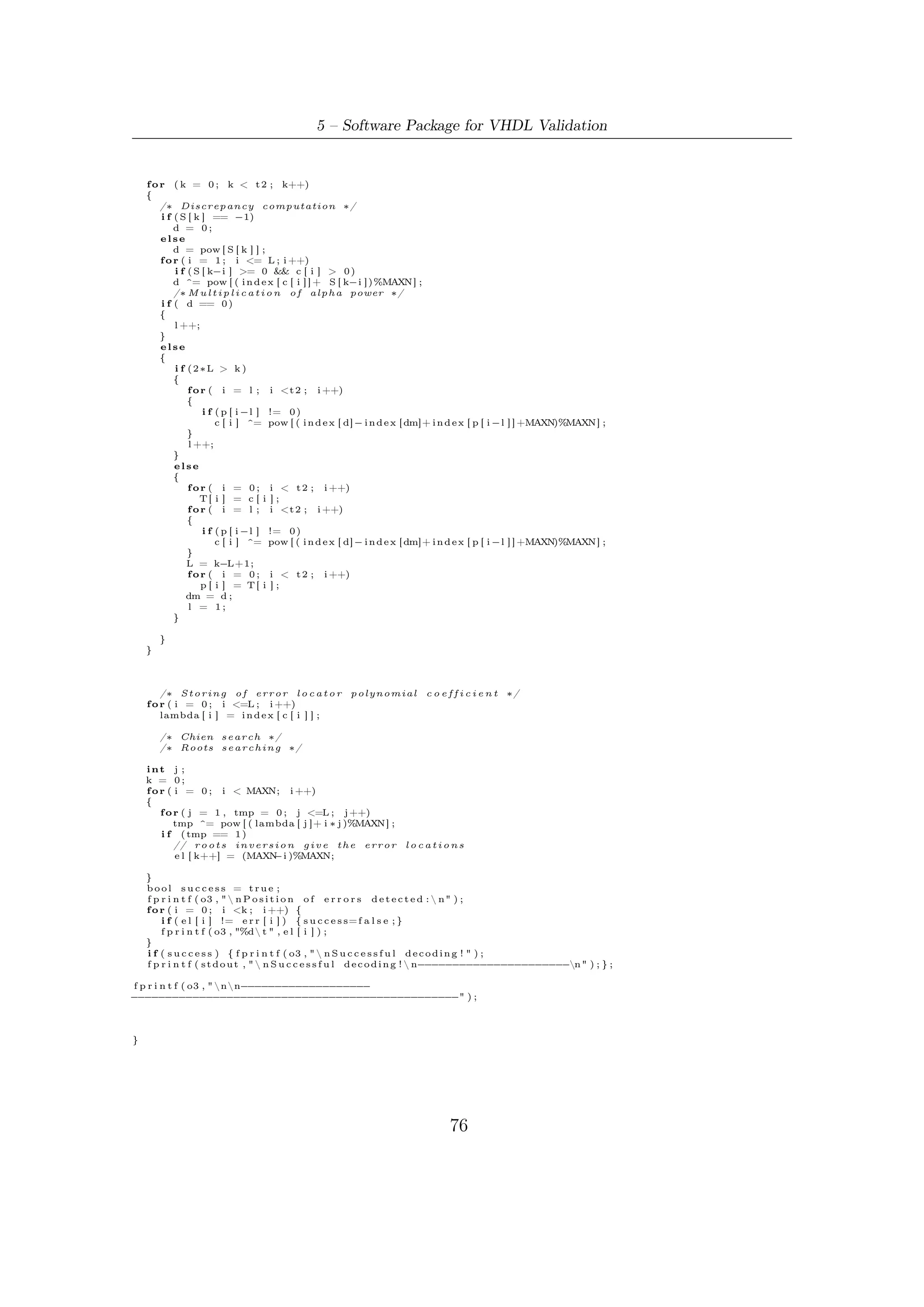
87. 5 – Software Package for VHDL Validation
transmission, are distributed as an uniform p.d.f. In practice, we shall simulate
a hard detection/corretion of errors.
An Error Detection Block and Syndrome Calculator: this block have the
simple task of computing syndromes associated to a received codeword. Clearly,
if any error is occurred then the codeword must be processed by decoder to try
correcting errors. Otherwise, no codewords are needed being corrected.
A Berlekamp Massey Decoder: when the number of errors is less or equal to
t, Berlekamp Massey algorithm and, in turn, the Chien search of roots can
correct the errors occurred during transmissions; in the other cases the decoder
state its failure in decoding.
In order to verify the functionality of all the algorithms, the positions of error
found at the decoder size are compared with the positions added by the error pattern
generation function. In case of any mismatch with the added error positions between
decoder and error generator, a decoding failure is stated. The result of each simulation
cycle can be saved onto a file, which can be indicated by the user.
5.5.1 Error Pattern Generation
Positions of errors are determined by using a C function (uniform01()) generating
a uniform distributed r.v. between [0, 1[, namely X; then
Y = nbch · X
represent the random error location, distributed uniformly between [0, nbch − 1].
5.5.2 The C Code
This section provides the code used in the simulation campaign (the implementation
of uniform01() will be omitted).
#include < s t d l i b . h>
#include <c o n i o . h>
#include <i o s t r e a m . h>
#include <t i m e . h>
#include <d o s . h>
#include < s t d i o . h>
#include < s t r i n g . h>
#include <f s t r e a m . h>
#include <math . h>
#d e f i n e MAXR 192 // max r b i t s
#d e f i n e P 8 // d e g r e e o f p a r a l l e l i s m
#d e f i n e MAXN ((1 < <16) −1) // p r i m i t i v e code l e n g t h
#d e f i n e MAXT 12 // Max c o r r e c t i v e c a p a c i t y
#d e f i n e DRIFT 0 // adding e x t r a e r r o r s
#i f n d e f TESTENC
#d e f i n e TESTDEC
#d e f i n e SERIAL
78

88. 5.5 – Software Robustness and Validation
#e n d i f
// ////////////////////////// M C O //////////////////////////////
A R
// I t r e t u r n s c o r r e c t i v e c a p a c i t y o f t h e code w i t h (n , k ) g i v e n //
// ///////////////////////////////////////////////////////////////
#d e f i n e t ( n , k ) ( ( ( n) −(k ) ) / ( 1 6 ) )
/∗ ∗∗∗∗∗∗∗∗∗∗∗∗∗∗∗∗∗∗∗∗∗∗∗∗∗∗∗∗∗∗∗∗∗∗∗∗∗∗∗∗∗∗∗∗∗∗∗∗∗∗∗∗∗∗∗∗∗∗∗∗∗∗∗∗∗∗∗∗∗∗∗∗∗∗ ∗/
/∗ ∗∗∗∗∗∗∗∗∗∗∗∗∗∗∗∗∗∗∗∗∗∗ G l o b a l V a r i a b l e ∗∗∗∗∗∗∗∗∗∗∗∗∗∗∗∗∗∗∗∗∗∗∗∗∗∗∗∗∗∗∗∗∗ ∗/
/∗ ∗∗∗∗∗∗∗∗∗∗∗∗∗∗∗∗∗∗∗∗∗∗∗∗∗∗∗∗∗∗∗∗∗∗∗∗∗∗∗∗∗∗∗∗∗∗∗∗∗∗∗∗∗∗∗∗∗∗∗∗∗∗∗∗∗∗∗∗∗∗∗∗∗ ∗/
i n t codeword [MAXN] ,
m e s s a g e [MAXN] ; // i n f o r m a t i o n bits
i n t Ap_n [MAXR] [MAXR] ; // (n−k ) rows , (n−k ) c o l
i n t Ap_k [MAXR] [MAXR] ; // 192 rows , 192 c o l
i n t C [MAXR] [ P ] ; // 192 rows , 8 c o l
i n t S [ (MAXT + DRIFT ) ∗ 2 ] ; // Syndrome v e c t o r
i n t e r r [MAXT+DRIFT ] ; // array o f random e r r o r l o c a t i o n
FILE ∗ o3 ;
/∗ ∗∗∗∗∗∗∗∗∗∗∗∗∗∗∗∗∗∗∗∗∗∗∗∗∗∗∗∗∗∗∗∗∗∗∗∗∗∗∗∗∗∗∗∗∗∗∗∗∗∗∗∗∗∗∗∗∗∗∗∗∗∗∗∗∗∗∗∗∗∗∗∗∗∗ ∗/
/∗ ∗∗∗∗∗∗∗∗∗∗∗∗∗∗∗∗∗∗∗∗∗∗ PN b i t s o u r c e ∗∗∗∗∗∗∗∗∗∗∗∗∗∗∗∗∗∗∗∗∗∗∗∗∗∗∗∗∗∗∗∗∗∗∗∗∗ ∗/
/∗ ∗∗∗∗∗∗∗∗∗∗∗∗∗∗∗∗∗∗∗∗∗∗∗∗∗∗∗∗∗∗∗∗∗∗∗∗∗∗∗∗∗∗∗∗∗∗∗∗∗∗∗∗∗∗∗∗∗∗∗∗∗∗∗∗∗∗∗∗∗∗∗∗∗ ∗/
i n t l f s r ( unsigned long i n t ∗ s e e d )
{
int b , c ;
b = ( ( ( ∗ s e e d ) & ( 1 << 3 1 ) ) >> 31 ) ;
c = ((∗ seed ) & 1) ^ ( ( ( ∗ s e e d ) & ( 1 << 1 ) ) >> 1 ) ^ ( ( ( ∗ s e e d ) & ( 1 << 2 1 ) ) >> 21 ) ^ b ;
( ∗ s e e d ) = ( ( ∗ s e e d ) << 1 ) | c;
return ( b ) ;
}
/∗ ∗∗∗∗∗∗∗∗∗∗∗∗∗∗∗∗∗∗∗∗∗∗∗∗∗∗∗∗∗∗∗∗∗∗∗∗∗∗∗∗∗∗∗∗∗∗∗∗∗∗∗∗∗∗∗∗∗∗∗∗∗∗∗∗∗∗∗∗∗∗∗∗∗∗ ∗/
/∗ ∗∗∗∗∗∗∗∗∗∗∗∗∗∗∗∗∗∗∗∗∗∗ Message g e n e r a t o r ∗∗∗∗∗∗∗∗∗∗∗∗∗∗∗∗∗∗∗∗∗∗∗∗∗∗∗∗∗∗∗∗∗ ∗/
/∗ ∗∗∗∗∗∗∗∗∗∗∗∗∗∗∗∗∗∗∗∗∗∗∗∗∗∗∗∗∗∗∗∗∗∗∗∗∗∗∗∗∗∗∗∗∗∗∗∗∗∗∗∗∗∗∗∗∗∗∗∗∗∗∗∗∗∗∗∗∗∗∗∗∗ ∗/
void message_gen ( i n t n , i n t k , unsigned long i n t ∗ seed )
{
int i ;
// Message b i t s pseudo random g e n e r a t i o n
f o r ( i=n −1; i >=n−k ; i −−)
message [ i ] = l f s r ( seed ) ;
// Zero padding
f o r ( i = 0 ; i < n−k ; i ++)
message [ i ] = 0 ;
}
/∗ ∗∗∗∗∗∗∗∗∗∗∗∗∗∗∗∗∗∗∗∗∗∗∗∗∗∗∗∗∗∗∗∗∗∗∗∗∗∗∗∗∗∗∗∗∗∗∗∗∗∗∗∗∗∗∗∗∗∗∗∗∗∗∗∗∗∗∗∗∗∗∗∗∗∗ ∗/
/∗ ∗∗∗∗∗∗∗∗∗∗∗∗∗∗∗∗∗∗∗∗∗∗ Polynomial Generators ∗∗∗∗∗∗∗∗∗∗∗∗∗∗∗∗∗∗∗∗∗∗∗∗∗∗∗∗ ∗/
/∗ ∗∗∗∗∗∗∗∗∗∗∗∗∗∗∗∗∗∗∗∗∗∗∗∗∗∗∗∗∗∗∗∗∗∗∗∗∗∗∗∗∗∗∗∗∗∗∗∗∗∗∗∗∗∗∗∗∗∗∗∗∗∗∗∗∗∗∗∗∗∗∗∗∗ ∗/
// Note : o n l y used by a l g o r i t h m e m u l a t i n g t h e s e r i a l a r c h i t e c t u r e (n−c l o c k c y c l e s )
const unsigned i n t g e n 1 2 [ ] =
{1 ,1 ,1 ,0 ,0 ,1 ,1 ,1 ,1 ,0 ,1 ,0 ,1 ,0 ,1 ,0 ,0 ,1 ,0 ,0 ,0 ,0 ,0 ,0 ,0 ,1 ,1 ,0 ,0 ,1 ,1 ,0 ,
1 ,1 ,1 ,0 ,1 ,1 ,1 ,1 ,1 ,0 ,1 ,0 ,0 ,0 ,0 ,1 ,1 ,1 ,1 ,0 ,0 ,0 ,1 ,0 ,1 ,1 ,0 ,0 ,0 ,0 ,0 ,0 ,
1 ,0 ,0 ,1 ,0 ,0 ,0 ,1 ,0 ,0 ,0 ,1 ,0 ,0 ,0 ,0 ,1 ,0 ,1 ,0 ,1 ,1 ,0 ,0 ,0 ,0 ,1 ,1 ,1 ,0 ,1 ,1 ,
0 ,0 ,0 ,1 ,1 ,0 ,1 ,1 ,0 ,0 ,1 ,1 ,0 ,1 ,0 ,0 ,1 ,1 ,1 ,1 ,0 ,0 ,1 ,1 ,0 ,0 ,0 ,0 ,1 ,0 ,1 ,0 ,
0 ,0 ,1 ,1 ,1 ,0 ,0 ,0 ,1 ,0 ,0 ,0 ,1 ,0 ,1 ,0 ,0 ,0 ,1 ,1 ,1 ,0 ,1 ,0 ,0 ,0 ,1 ,0 ,0 ,0 ,0 ,1 ,
1 ,1 ,0 ,0 ,0 ,0 ,0 ,1 ,0 ,1 ,1 ,1 ,0 ,0 ,0 ,0 ,0 ,1 ,1 ,0 ,0 ,1 ,0 ,0 ,0 ,1 ,1 ,1 ,0 ,0 ,1 ,0 ,
1};
// i . e . gen ( x ) = a_0∗ x^0 + a_1∗ x^1 + . . . + a_( r −1)∗x ^( r −1) + a_r∗ x^r
const unsigned i n t gen10 [ ] =
{1 ,0 ,0 ,0 ,1 ,0 ,0 ,1 ,1 ,0 ,1 ,0 ,0 ,1 ,1 ,0 ,1 ,1 ,0 ,1 ,1 ,1 ,0 ,1 ,0 ,0 ,0 ,1 ,1 ,1 ,0 ,1 ,
1 ,0 ,0 ,0 ,0 ,0 ,0 ,0 ,1 ,1 ,0 ,0 ,0 ,1 ,0 ,0 ,1 ,0 ,0 ,0 ,1 ,0 ,1 ,1 ,1 ,1 ,1 ,1 ,0 ,1 ,1 ,1 ,
1 ,1 ,0 ,0 ,0 ,0 ,0 ,0 ,1 ,1 ,1 ,0 ,1 ,0 ,1 ,0 ,0 ,0 ,0 ,1 ,1 ,1 ,1 ,0 ,0 ,1 ,0 ,1 ,0 ,1 ,1 ,0 ,
1 ,1 ,1 ,1 ,1 ,0 ,0 ,0 ,1 ,1 ,0 ,0 ,1 ,1 ,0 ,0 ,0 ,1 ,0 ,1 ,0 ,1 ,0 ,0 ,0 ,0 ,1 ,1 ,1 ,1 ,1 ,1 ,
1 ,0 ,1 ,1 ,0 ,1 ,1 ,1 ,0 ,0 ,1 ,1 ,0 ,0 ,0 ,0 ,1 ,0 ,1 ,0 ,1 ,0 ,0 ,0 ,0 ,0 ,0 ,0 ,0 ,1 ,1 ,0 ,
1};
const unsigned i n t gen8 [ ] =
{1 ,1 ,0 ,1 ,0 ,1 ,0 ,0 ,0 ,1 ,1 ,0 ,0 ,1 ,1 ,0 ,1 ,0 ,0 ,1 ,1 ,1 ,1 ,1 ,0 ,0 ,1 ,0 ,0 ,0 ,0 ,0 ,
79

89. 5 – Software Package for VHDL Validation
1 ,0 ,1 ,0 ,1 ,1 ,1 ,0 ,1 ,0 ,1 ,1 ,0 ,1 ,1 ,0 ,0 ,0 ,1 ,1 ,1 ,1 ,1 ,1 ,1 ,0 ,0 ,1 ,1 ,0 ,0 ,0 ,
1 ,0 ,1 ,1 ,1 ,1 ,0 ,1 ,1 ,1 ,1 ,0 ,1 ,0 ,0 ,1 ,1 ,1 ,1 ,0 ,0 ,1 ,0 ,0 ,1 ,0 ,0 ,0 ,1 ,1 ,1 ,0 ,
1 ,1 ,1 ,1 ,1 ,0 ,1 ,0 ,1 ,0 ,1 ,0 ,0 ,1 ,0 ,0 ,1 ,1 ,1 ,0 ,0 ,0 ,0 ,0 ,0 ,0 ,1 ,1 ,1 ,0 ,0 ,0 ,
1};
/∗ ∗∗∗∗∗∗∗∗∗∗∗∗∗∗∗∗∗∗∗∗∗∗∗∗∗∗∗∗∗∗∗∗∗∗∗∗∗∗∗∗∗∗∗∗∗∗∗∗∗∗∗∗∗∗∗∗∗∗∗∗∗∗∗∗∗∗∗∗∗∗∗∗∗∗ ∗/
/∗ ∗∗∗∗∗∗∗∗∗∗∗∗∗∗∗∗∗∗∗∗∗∗ S e r i a l BCH encoder ∗∗∗∗∗∗∗∗∗∗∗∗∗∗∗∗∗∗∗∗∗∗∗∗∗∗∗∗∗∗∗ ∗/
/∗ ∗∗∗∗∗∗∗∗∗∗∗∗∗∗∗∗∗∗∗∗∗∗∗∗∗∗∗∗∗∗∗∗∗∗∗∗∗∗∗∗∗∗∗∗∗∗∗∗∗∗∗∗∗∗∗∗∗∗∗∗∗∗∗∗∗∗∗∗∗∗∗∗∗ ∗/
void BCH_s_enc ( i n t n , int k )
{
const unsigned i n t ∗ g ;
int ∗ reg ;
i n t mem, app , i , j ;
/∗ ∗∗∗∗∗∗∗∗∗∗∗∗∗∗ Mode S e l e c t i o n ( t−e r r o r−c o r r e c t i o n ) ∗∗∗∗∗∗∗∗∗∗∗∗∗∗∗∗∗∗∗∗∗∗ ∗/
switch ( n−k ) {
case 1 9 2 :
g = gen12 ;
r e g = ( i n t ∗ ) c a l l o c ( n−k , s i z e o f ( i n t ) ) ;
break ;
case 1 6 0 :
g = gen10 ;
r e g = ( i n t ∗ ) c a l l o c ( n−k , s i z e o f ( i n t ) ) ;
break ;
case 1 2 8 :
g = gen8 ;
r e g = ( i n t ∗ ) c a l l o c ( n−k , s i z e o f ( i n t ) ) ;
break ;
default :
f p r i n t f ( s t d o u t , " E r r o r : s i m u l a t i o n a b o r t e d ! n" ) ;
f p r i n t f ( s t d o u t , " P l e a s e i n s e r t a n−k c o u p l e p r o v i d e d by DVB−S2 FECn" ) ;
exit (0);
}
/∗ ∗∗∗∗∗∗∗∗∗∗∗∗∗∗∗∗∗∗∗∗∗∗ Encoding s e r i a l a l g o r i t h m ∗∗∗∗∗∗∗∗∗∗∗∗∗∗∗∗∗∗∗∗∗∗∗∗∗∗∗∗∗∗∗ ∗/
/∗ ∗∗∗∗∗∗∗∗∗∗∗∗∗∗∗∗∗∗∗∗∗∗∗∗∗ n c l o c k t i c k s ∗∗∗∗∗∗∗∗∗∗∗∗∗∗∗∗∗∗∗∗∗∗∗∗∗∗∗∗∗∗∗∗∗∗∗∗∗ ∗/
/∗ ∗∗∗∗∗∗∗∗∗∗∗∗∗∗∗∗∗∗∗∗∗∗∗∗ Computing remainder ∗∗∗∗∗∗∗∗∗∗∗∗∗∗∗∗∗∗∗∗∗∗∗∗∗∗∗∗∗∗∗∗∗ ∗/
f o r ( i=n −1; i >=0; i −−)
{
mem=r e g [ n−k − 1 ] ;
f o r ( j=n−k −2; j >=0; j −−)
{
app=mem & g [ j + 1 ] ;
r e g [ j +1]= r e g [ j ] ^ app ;
}
r e g [ 0 ] = m e s s a g e [ i ] ^ (mem & g [ 0 ] ) ;
}
/∗ ∗∗∗∗∗∗∗∗∗∗∗∗∗∗∗∗∗∗∗∗∗∗ Codeword i n s y s t e m a t i c form ∗∗∗∗∗∗∗∗∗∗∗∗∗∗∗∗∗∗∗∗∗∗∗∗∗∗∗∗∗∗∗ ∗/
f o r ( i=n −1; i >=n−k ; i −−)
codeword [ i ] = m e s s a g e [ i ] ;
f o r ( i=n−k −1; i >=0; i −−)
codeword [ i ] = r e g [ i ] ;
f r e e ( reg ) ;
}
/∗ ∗∗∗∗∗∗∗∗∗∗∗∗∗∗∗∗∗∗∗∗∗∗∗∗∗∗∗∗∗∗∗∗∗∗∗∗∗∗∗∗∗∗∗∗∗∗∗∗∗∗∗∗∗∗∗∗∗∗∗∗∗∗∗∗∗∗∗∗∗∗∗∗∗∗ ∗/
/∗ ∗∗∗∗∗∗∗∗∗∗∗∗∗∗∗∗∗∗∗∗∗∗ Loading m a t r i c e s r o u t i n e ∗∗∗∗∗∗∗∗∗∗∗∗∗∗∗∗∗∗∗∗∗∗∗∗∗∗ ∗/
/∗ ∗∗∗∗∗∗∗∗∗∗∗∗∗∗∗∗∗∗∗∗∗∗∗∗∗∗∗∗∗∗∗∗∗∗∗∗∗∗∗∗∗∗∗∗∗∗∗∗∗∗∗∗∗∗∗∗∗∗∗∗∗∗∗∗∗∗∗∗∗∗∗∗∗ ∗/
void l o a d _ m a t r i c e s ( i n t n , i n t k )
{
FILE ∗input_Ap_k , ∗input_C , ∗input_Ap_n ;
int i , j ;
/∗ ∗∗∗∗∗∗∗∗∗∗∗∗∗∗∗∗∗∗∗∗∗∗ Mode S e l e c t i o n ( t−e r r o r−c o r r e c t i o n ) ∗∗∗∗∗∗∗∗∗∗∗∗∗∗∗∗∗∗∗∗∗∗ ∗/
switch ( n−k ) {
case 1 9 2 :
input_Ap_k = f o p e n ( " M a t r i c e s /ADVBS2_nclk_t12 . t x t " , " r " ) ;
input_Ap_n = f o p e n ( " M a t r i c e s /ADVBS2_nclk_t12 . t x t " , " r " ) ;
input_C = f o p e n ( " M a t r i c e s /CDVBS2_kclk_t12 . t x t " , " r " ) ;
break ;
case 1 6 0 :
80

90. 5.5 – Software Robustness and Validation
input_Ap_k = f o p e n ( " M a t r i c e s /ADVBS2_kclk_t10 . t x t " , " r " ) ;
input_Ap_n = f o p e n ( " M a t r i c e s /ADVBS2_nclk_t10 . t x t " , " r " ) ;
input_C = f o p e n ( " M a t r i c e s /CDVBS2_kclk_t10 . t x t " , " r " ) ;
break ;
case 1 2 8 :
input_Ap_k = f o p e n ( " M a t r i c e s /ADVBS2_kclk_t8 . t x t " , " r " ) ;
input_Ap_n = f o p e n ( " M a t r i c e s /ADVBS2_nclk_t8 . t x t " , " r " ) ;
input_C = f o p e n ( " M a t r i c e s /CDVBS2_kclk_t8 . t x t " , " r " ) ;
break ;
default :
f p r i n t f ( s t d o u t , " E r r o r : l o a d i n g o f m a t r i c e s f a i l e d ! n" ) ;
f p r i n t f ( s t d o u t , " P l e a s e i n s e r t a n−k c o u p l e p r o v i d e d by DVB −S2 FECn" ) ;
exit (0);
}
/∗ ∗∗∗∗∗∗∗∗∗∗∗∗∗∗∗∗∗∗∗∗ Loading matrix Ap_n ∗∗∗∗∗∗∗∗∗∗∗∗∗∗∗∗∗∗∗∗∗∗∗∗∗∗∗∗∗∗∗∗∗∗ ∗/
/////////// Note : ONLY t h i s matrix s i z e i s v a r i a b l e //////////////////////////
f o r ( i =0; i <n−k ; i ++){
f o r ( j =0; j <n−k ; j ++){
// f s c a n f ( input_Ap_k,"%d t " ,&(Ap_k [ i ] [ j ] ) ) ;
f s c a n f ( input_Ap_n , "%d t " ,&(Ap_n [ i ] [ j ] ) ) ;
//power_A [ i ] [ j ] = load_i ;
}
// f s c a n f ( input_Ap_k , " n " ) ;
f s c a n f ( input_Ap_n , " n" ) ;
}
/∗ ∗∗∗∗∗∗∗∗∗∗∗∗∗∗∗∗∗∗∗∗ Loading matrix Ap_k ∗∗∗∗∗∗∗∗∗∗∗∗∗∗∗∗∗∗∗∗∗∗∗∗∗∗∗∗∗∗∗∗∗∗ ∗/
f o r ( i =0; i < MAXR; i ++)
f o r ( j =0; j < MAXR; j ++)
f s c a n f ( input_Ap_k , "%d t " , &(Ap_k [ i ] [ j ] ) ) ;
f s c a n f ( input_Ap_k , " n" ) ;
/∗ ∗∗∗∗∗∗∗∗∗∗∗∗∗∗∗∗∗∗∗∗ Loading matrix C ∗∗∗∗∗∗∗∗∗∗∗∗∗∗∗∗∗∗∗∗∗∗∗∗∗∗∗∗∗∗∗∗∗∗ ∗/
f o r ( i =0; i < MAXR; i ++)
{
f o r ( j =0; j <P ; j ++)
{
f s c a n f ( input_C , "%d t " ,&(C [ i ] [ j ] ) ) ;
//comb_C[ i ] [ j ] = load_c ;
}
fscanf ( input_C , " n" ) ;
}
f c l o s e ( input_C ) ;
f c l o s e ( input_Ap_n ) ;
f c l o s e ( input_Ap_k ) ;
}
/∗ ∗∗∗∗∗∗∗∗∗∗∗∗∗∗∗∗∗∗∗∗∗∗∗∗∗∗∗∗∗∗∗∗∗∗∗∗∗∗∗∗∗∗∗∗∗∗∗∗∗∗∗∗∗∗∗∗∗∗∗∗∗∗∗∗∗∗∗∗∗∗ ∗/
/∗ ∗∗∗∗∗∗∗∗∗∗ Combinatorial b l o c k s emulation ∗∗∗∗∗∗∗∗∗∗∗∗∗∗∗∗∗∗∗∗∗∗∗∗∗∗∗ ∗/
/∗ ∗∗∗∗∗∗∗∗∗∗∗∗∗∗∗∗∗∗∗∗∗∗∗∗∗∗∗∗∗∗∗∗∗∗∗∗∗∗∗∗∗∗∗∗∗∗∗∗∗∗∗∗∗∗∗∗∗∗∗∗∗∗∗∗∗∗∗∗∗ ∗/
/∗ ∗∗∗∗∗∗∗∗∗∗∗∗∗∗∗∗∗∗∗∗∗∗∗∗∗∗∗∗∗∗∗∗∗∗∗∗∗∗∗∗∗∗∗∗∗∗∗∗∗∗∗∗∗∗∗∗∗∗∗∗∗∗∗∗∗∗∗∗∗∗ ∗/
/∗ ∗∗∗∗∗∗∗∗∗∗∗∗∗∗∗∗∗ I n p u t comb network ∗∗∗∗∗∗∗∗∗∗∗∗∗∗∗∗∗∗∗∗∗∗∗∗∗∗∗∗∗∗∗ ∗/
/∗ ∗∗∗∗∗∗∗∗∗∗∗∗∗∗∗∗∗∗∗∗∗∗∗∗∗∗∗∗∗∗∗∗∗∗∗∗∗∗∗∗∗∗∗∗∗∗∗∗∗∗∗∗∗∗∗∗∗∗∗∗∗∗∗∗∗∗∗∗∗ ∗/
i n t comb_c ( i n t i n d e x , int ∗ input )
{
i n t out , f , i n d ;
o u t =0;
i n d=P−1;
f o r ( f =0; f <P ; f ++)
{
o u t= o u t ^ ( (C [ i n d e x ] [ f ] ) & ( i n p u t [ f ] ) ) ;
ind −−;
}
return ( o u t ) ;
81

91. 5 – Software Package for VHDL Validation
}
/∗ ∗∗∗∗∗∗∗∗∗∗∗∗∗∗∗∗∗∗∗∗∗∗∗∗∗∗∗∗∗∗∗∗∗∗∗∗∗∗∗∗∗∗∗∗∗∗∗∗∗∗∗∗∗∗∗∗∗∗∗∗∗∗∗∗∗∗∗∗∗∗ ∗/
/∗ ∗∗∗∗∗∗∗∗∗∗∗∗∗∗∗∗∗ S t a t e comb network ∗∗∗∗∗∗∗∗∗∗∗∗∗∗∗∗∗∗∗∗∗∗∗∗∗∗∗∗∗∗∗ ∗/
/∗ ∗∗∗∗∗∗∗∗∗∗∗∗∗∗∗∗∗∗∗∗∗∗∗∗∗∗∗∗∗∗∗∗∗∗∗∗∗∗∗∗∗∗∗∗∗∗∗∗∗∗∗∗∗∗∗∗∗∗∗∗∗∗∗∗∗∗∗∗∗ ∗/
i n t comb_n ( i n t i n d e x , i n t r , int ∗ reg_old )
{
i n t out , f ;
o u t =0;
f o r ( f =0; f <P ; f ++)
{
o u t=o u t ^(Ap_n [ i n d e x ] [ r−f −1] & r e g _ o l d [ r−f − 1 ] ) ;
}
return ( o u t ) ;
}
i n t comb_k ( i n t i n d e x , int ∗ reg_old )
{
i n t out , f ;
o u t =0;
f o r ( f =0; f <P ; f ++)
{
o u t=o u t ^(Ap_k [ i n d e x ] [ MAXR −1] & r e g _ o l d [MAXR − 1 ] ) ;
−f −f
}
return ( o u t ) ;
}
/∗ ∗∗∗∗∗∗∗∗∗∗∗∗∗∗∗∗∗∗∗∗∗∗∗∗∗∗∗∗∗∗∗∗∗∗∗∗∗∗∗∗∗∗∗∗∗∗∗∗∗∗∗∗∗∗∗∗∗∗∗∗∗∗∗∗∗∗∗∗∗∗∗∗∗∗ ∗/
/∗ ∗∗∗∗∗∗∗∗∗∗∗∗∗∗∗∗∗∗∗∗∗∗ BCH p a r e l l e l encoder ∗∗∗∗∗∗∗∗∗∗∗∗∗∗∗∗∗∗∗∗∗∗∗∗∗∗∗∗∗∗ ∗/
/∗ ∗∗∗∗∗∗∗∗∗∗∗∗∗∗∗∗∗∗∗∗∗∗ n c l o c k t i c k s ∗∗∗∗∗∗∗∗∗∗∗∗∗∗∗∗∗∗∗∗∗∗∗∗∗∗∗∗∗∗ ∗/
/∗ ∗∗∗∗∗∗∗∗∗∗∗∗∗∗∗∗∗∗∗∗∗∗∗∗∗∗∗∗∗∗∗∗∗∗∗∗∗∗∗∗∗∗∗∗∗∗∗∗∗∗∗∗∗∗∗∗∗∗∗∗∗∗∗∗∗∗∗∗∗∗∗∗∗ ∗/
void BCHnclk_par ( i n t n , i n t k )
{
int c l o c k _ t i c k s ;
int ∗ reg , ∗ reg_old ;
int input [P ] ; // p a r a l l e l input bits
/∗ ∗∗∗∗∗∗∗∗∗∗∗∗∗∗ Mode S e l e c t i o n ( t−e r r o r−c o r r e c t i o n ) ∗∗∗∗∗∗∗∗∗∗∗∗∗∗∗∗∗∗∗∗∗∗ ∗/
switch ( n−k ) {
case 1 9 2 :
r e g = ( i n t ∗ ) c a l l o c ( n−k , s i z e o f ( i n t ) ) ;
r e g _ o l d = ( i n t ∗ ) c a l l o c ( n−k , s i z e o f ( i n t ) ) ;
break ;
case 1 6 0 :
r e g = ( i n t ∗ ) c a l l o c ( n−k , s i z e o f ( i n t ) ) ;
r e g _ o l d = ( i n t ∗ ) c a l l o c ( n−k , s i z e o f ( i n t ) ) ;
break ;
case 1 2 8 :
r e g = ( i n t ∗ ) c a l l o c ( n−k , s i z e o f ( i n t ) ) ;
r e g _ o l d = ( i n t ∗ ) c a l l o c ( n−k , s i z e o f ( i n t ) ) ;
break ;
default :
f p r i n t f ( s t d o u t , " E r r o r : s i m u l a t i o n a b o r t e d ! n" ) ;
f p r i n t f ( s t d o u t , " P l e a s e i n s e r t a n−k c o u p l e p r o v i d e d by DVB−S2 FECn" ) ;
exit (0);
}
/// Computation o f c l o c k t i c k s r e q u i r e d t o compute t h e remainder a f t e r d i v i s i o n ////
c l o c k _ t i c k s = n/P ;
/∗ ∗∗∗∗∗∗∗∗∗∗∗∗∗∗∗∗∗∗∗∗∗∗∗∗ Computing remainder ∗∗∗∗∗∗∗∗∗∗∗∗∗∗∗∗∗∗∗∗∗∗∗∗∗∗∗∗∗∗∗∗∗ ∗/
i n t z =0;
f o r ( i n t i =0; i <c l o c k _ t i c k s ; i ++)
{
///// r e f r e s h o f s t a t e /////// ///////
f o r ( i n t m=0; m <n−k ; m++)
r e g _ o l d [m]= r e g [m ] ;
82

92. 5.5 – Software Robustness and Validation
// /////////////////////////////////////
/////// l o a d i n g o f p a r a l l e l i n p u t //////
f o r ( i n t c o u n t=P−1; count >=0; count −−)
{
z++;
i n p u t [ c o u n t ] = m e s s a g e [ n−z ] ;
}
// /////////////////////////////////////////
/// Computing o f n e x t v a l u e s o f s t a t e /////
i f ( c l o c k _ t i c k s >0)
{
f o r (m=0; m <n−k ; m++)
{
i f (m<P)
r e g [m] = i n p u t [m] ^ comb_n (m, n−k , r e g _ o l d ) ;
else
r e g [m] = comb_n (m, n−k , r e g _ o l d )^ r e g _ o l d [ m−P ] ;
}
}
// ///////////////////////////////////////////
}
/∗ ∗∗∗∗∗∗∗∗∗∗∗∗∗∗∗∗∗∗∗∗∗∗∗∗∗∗∗∗∗∗∗∗∗∗∗∗∗∗∗∗∗∗∗∗∗∗∗∗∗∗∗∗∗∗∗∗∗∗∗∗∗∗∗∗∗∗∗∗∗∗∗∗∗∗∗∗∗∗∗∗∗∗ ∗/
/∗ ∗∗∗∗∗∗∗∗∗∗∗∗∗∗∗∗∗∗∗∗∗∗ Codeword i n s y s t e m a t i c form ∗∗∗∗∗∗∗∗∗∗∗∗∗∗∗∗∗∗∗∗∗∗∗∗∗∗∗∗∗∗∗ ∗/
f o r ( i=n −1; i >n−k −1; i −−)
codeword [ i ] = m e s s a g e [ i ] ;
f o r ( i=n−k −1; i >=0; i −−)
codeword [ i ] = reg [ i ] ;
}
/∗ ∗∗∗∗∗∗∗∗∗∗∗∗∗∗∗∗∗∗∗∗∗∗∗∗∗∗∗∗∗∗∗∗∗∗∗∗∗∗∗∗∗∗∗∗∗∗∗∗∗∗∗∗∗∗∗∗∗∗∗∗∗∗∗∗∗∗∗∗∗∗∗∗∗∗ ∗/
/∗ ∗∗∗∗∗∗∗∗∗∗∗∗∗∗∗∗∗∗∗∗∗∗ BCH p a r e l l e l encoder ∗∗∗∗∗∗∗∗∗∗∗∗∗∗∗∗∗∗∗∗∗∗∗∗∗∗∗∗∗∗ ∗/
/∗ ∗∗∗∗∗∗∗∗∗∗∗∗∗∗∗∗∗∗∗∗∗∗ k c l o c k t i c k s ∗∗∗∗∗∗∗∗∗∗∗∗∗∗∗∗∗∗∗∗∗∗∗∗∗∗∗∗∗∗ ∗/
/∗ ∗∗∗∗∗∗∗∗∗∗∗∗∗∗∗∗∗∗∗∗∗∗∗∗∗∗∗∗∗∗∗∗∗∗∗∗∗∗∗∗∗∗∗∗∗∗∗∗∗∗∗∗∗∗∗∗∗∗∗∗∗∗∗∗∗∗∗∗∗∗∗∗∗ ∗/
void BCHkclk_par ( i n t n , i n t k )
{
int c l o c k _ t i c k s ;
int ∗ reg , ∗ reg_old ;
i n t o f f s e t ,m;
int input [P ] ; // p a r a l l e l input bits
/∗ ∗∗∗∗∗∗∗∗∗∗∗∗∗∗ Mode S e l e c t i o n ( t−e r r o r−c o r r e c t i o n ) ∗∗∗∗∗∗∗∗∗∗∗∗∗∗∗∗∗∗∗∗∗∗ ∗/
switch ( n−k ) {
case 1 9 2 :
r e g = ( i n t ∗ ) c a l l o c (MAXR, s i z e o f ( i n t ) ) ;
r e g _ o l d = ( i n t ∗ ) c a l l o c (MAXR, s i z e o f ( i n t ) ) ;
o f f s e t = MAXR−192;
break ;
case 1 6 0 :
r e g = ( i n t ∗ ) c a l l o c (MAXR, s i z e o f ( i n t ) ) ;
r e g _ o l d = ( i n t ∗ ) c a l l o c (MAXR, s i z e o f ( i n t ) ) ;
o f f s e t = MAXR − 1 6 0 ;
break ;
case 1 2 8 :
r e g = ( i n t ∗ ) c a l l o c (MAXR, s i z e o f ( i n t ) ) ;
r e g _ o l d = ( i n t ∗ ) c a l l o c (MAXR, s i z e o f ( i n t ) ) ;
o f f s e t = MAXR−128;
break ;
default :
f p r i n t f ( s t d o u t , " E r r o r : e n c o d i n g a b o r t e d ! n" ) ;
f p r i n t f ( s t d o u t , " P l e a s e i n s e r t a n−k c o u p l e p r o v i d e d by DVB−S2 FECn" ) ;
exit (0);
}
/// Computation o f c l o c k t i c k s r e q u i r e d t o compute t h e remainder a f t e r d i v i s i o n ////
c l o c k _ t i c k s = k /P ;
/∗ ∗∗∗∗∗∗∗∗∗∗∗∗∗∗∗∗∗∗∗∗∗∗∗∗ Computing remainder ∗∗∗∗∗∗∗∗∗∗∗∗∗∗∗∗∗∗∗∗∗∗∗∗∗∗∗∗∗∗∗∗∗ ∗/
i n t z =0;
f o r ( i n t i =0; i <c l o c k _ t i c k s ; i ++)
{
f o r (m=0; m < MAXR; m++)
83

93. 5 – Software Package for VHDL Validation
r e g _ o l d [m]= r e g [m ] ;
f o r ( i n t c o u n t=P−1; count >=0; count −−)
{
z++;
i n p u t [ c o u n t ] = m e s s a g e [ n−z ] ;
}
if ( c l o c k _ t i c k s >0)
{
f o r (m=0; m MAXR; m++)
<
{
i f (m<P)
r e g [m] = ( comb_c (m, i n p u t ) ) ^ ( comb_k (m, r e g _ o l d ) ) ;
else
r e g [m] = ( comb_c (m, i n p u t ) ) ^ ( comb_k (m, r e g _ o l d ) ) ^ ( r e g _ o l d [ m−(P ) ] ) ;
}
}
}
/∗ ∗∗∗∗∗∗∗∗∗∗∗∗∗∗∗∗∗∗∗∗∗∗ Codeword i n s y s t e m a t i c form ∗∗∗∗∗∗∗∗∗∗∗∗∗∗∗∗∗∗∗∗∗∗∗∗∗∗∗∗∗∗∗ ∗/
f o r ( i=n −1; i >n−k −1; i −−)
codeword [ i ] = m e s s a g e [ i ] ;
f o r ( i=n−k −1; i >=0 ; i −−)
codeword [ i ] = r e g [ i+ o f f s e t ] ;
/∗ Check v a l u e s o f r e g i s t e r
FILE ∗ de ;
de = fopen (" d e b u g k c l k . t x t " ,"w" ) ;
f o r ( i = MAXR −1; i >=0; i −−)
f p r i n t f ( de ,"%dn" , r e g [ i ] ) ;
∗/
}
/∗ ∗∗∗∗∗∗∗∗∗∗∗∗∗∗∗∗∗∗∗∗∗∗∗∗∗∗∗∗∗∗∗∗∗∗∗∗∗∗∗∗∗∗∗∗∗∗∗∗∗∗∗∗∗∗∗∗∗∗∗∗∗∗∗∗∗∗∗∗∗∗∗∗∗∗ ∗/
/∗ ∗∗∗∗∗∗∗∗∗∗∗∗∗∗∗∗∗∗∗∗∗∗ Creation o f GF(2^m) ∗∗∗∗∗∗∗∗∗∗∗∗∗∗∗∗∗∗∗∗∗∗∗∗∗∗∗∗∗∗ ∗/
/∗ ∗∗∗∗∗∗∗∗∗∗∗∗∗∗∗∗∗∗∗∗∗∗ u s e f u l t a b l e s ∗∗∗∗∗∗∗∗∗∗∗∗∗∗∗∗∗∗∗∗∗∗∗∗∗∗∗∗∗∗ ∗/
/∗ ∗∗∗∗∗∗∗∗∗∗∗∗∗∗∗∗∗∗∗∗∗∗∗∗∗∗∗∗∗∗∗∗∗∗∗∗∗∗∗∗∗∗∗∗∗∗∗∗∗∗∗∗∗∗∗∗∗∗∗∗∗∗∗∗∗∗∗∗∗∗∗∗∗ ∗/
void g f F i e l d ( i n t m, // Base 2 l o g a r i t h m o f c a r d i n a l i t y o f t h e F i e l d
i n t p o l y , // p r i m i t i v e p o l y n o m i a l o f t h e F i e l d i n decimal form
i n t ∗∗ powOfAlpha , i n t ∗∗ i n d e x A l p h a )
{
int reg , // t h i s i n t e g e r o f 32 b i t s , masked by a sequence o f m ones ,
// c o n t a i n s t h e e l e m e n t s o f G a l o i s F i e l d
tmp , i ;
// sequence o f m ones
i n t mask = (1<<m) −1; // 1(m) B i t Masking
// A l l o c a t i o n and i n i t i a l i z a t i o n o f t h e t a b l e s o f t h e G a l o i s F i e l d
∗ powOfAlpha = ( i n t ∗ ) c a l l o c ((1<<m) −2 , s i z e o f ( i n t ) ) ;
∗ i n d e x A l p h a = ( i n t ∗ ) c a l l o c ((1<<m) −1 , s i z e o f ( i n t ) ) ;
( ∗ powOfAlpha ) [ 0 ] = 1 ;
( ∗ i n d e x A l p h a ) [ 0 ] = − 1 ; // we s e t −1
(∗ indexAlpha ) [ 1 ] = 0 ;
f o r ( i = 0 , r e g = 1 ; i < (1<<m) −2; i ++)
{
tmp = ( i n t ) ( r e g & (1<<(m− 1 ) ) ) ; // Get t h e MSB
reg < <= 1 ; // R e g i s t e r s h i f t e d
i f ( tmp ) { //
r e g ^= p o l y ;
//
r e g &= mask ;
}
// Step−by−s t e p w r i t i n g o f t h e t a b l e s
( ∗ powOfAlpha ) [ i +1] = ( i n t ) r e g ;
( ∗ i n d e x A l p h a ) [ ( i n t ) r e g ] = i +1;
}
}
/∗ ∗∗∗∗∗∗∗∗∗∗∗∗∗∗∗∗∗∗∗∗∗∗∗∗∗∗∗∗∗∗∗∗∗∗∗∗∗∗∗∗∗∗∗∗∗∗∗∗∗∗∗∗∗∗∗∗∗∗∗∗∗∗∗∗∗∗∗∗∗∗∗∗∗∗ ∗/
/∗ ∗∗∗∗∗∗∗∗∗∗∗∗∗∗∗∗∗∗∗∗∗∗ Error d e t e c t i o n ∗∗∗∗∗∗∗∗∗∗∗∗∗∗∗∗∗∗∗∗∗∗∗∗∗∗∗∗∗∗ ∗/
/∗ ∗∗∗∗∗∗∗∗∗∗∗∗∗∗∗∗∗∗∗∗∗∗∗∗∗∗∗∗∗∗∗∗∗∗∗∗∗∗∗∗∗∗∗∗∗∗∗∗∗∗∗∗∗∗∗∗∗∗∗∗∗∗∗∗∗∗∗∗∗∗∗∗∗ ∗/
84

94. 5.5 – Software Robustness and Validation
bool e r r o r _ d e t e c t i o n ( i n t ∗pow , int ∗ index , int t )
{
b o o l syn = f a l s e ;
f o r ( i n t i = 0 ; i < t ∗ 2 ; i ++)
{
S [ i ] = 0;
f o r ( i n t j = 0 ; j < MAXN; j ++){
i f ( codeword [ j ] )
S [ i ] ^= pow [ ( ( i +1)∗ j )%MAXN] ;
}
i f ( ( S [ i ] = i n d e x [ S [ i ] ] ) != −1)
syn = t r u e ;
}
return syn ;
}
/∗ ∗∗∗∗∗∗∗∗∗∗∗∗∗∗∗∗∗∗∗∗∗∗∗∗∗∗∗∗∗∗∗∗∗∗∗∗∗∗∗∗∗∗∗∗∗∗∗∗∗∗∗∗∗∗∗∗∗∗∗∗∗∗∗∗∗∗∗∗∗∗∗∗∗∗ ∗/
/∗ ∗∗∗∗∗∗∗∗∗∗∗∗∗∗∗∗∗∗∗∗∗∗ Error c o r r e c t i o n ∗∗∗∗∗∗∗∗∗∗∗∗∗∗∗∗∗∗∗∗∗∗∗∗∗∗∗∗∗∗ ∗/
/∗ ∗∗∗∗∗∗∗∗∗∗∗∗∗∗∗∗∗∗∗∗∗∗∗∗∗∗∗∗∗∗∗∗∗∗∗∗∗∗∗∗∗∗∗∗∗∗∗∗∗∗∗∗∗∗∗∗∗∗∗∗∗∗∗∗∗∗∗∗∗∗∗∗∗ ∗/
void B e r l M a s s ( // i n t ∗S , // array o f syndrome i n e x p o n e n t i a l n o t a t i o n
i n t t2 , // l e n g t h o f array S
i n t ∗pow ,
int ∗ index )
{
int k , L , l , i ;
i n t d , dm, tmp ;
i n t ∗T, ∗ c , ∗p , ∗ lambda , ∗ e l ;
// A l l o c a t i o n and i n i t i a l i z a t i o n
// Auto−R e g r e s s i v e −F i l t e r c o e f f i c i e n t s computed a t t h e p r e v i o u s s t e p
p = ( i n t ∗ ) c a l l o c ( t2 , s i z e o f ( i n t ) ) ;
// Auto−R e g r e s s i v e −F i l t e r c o e f f i c i e n t s computed a t t h e c u r r e n t s t e p
c = ( i n t ∗ ) c a l l o c ( t2 , s i z e o f ( i n t ) ) ;
// Temporary array
T = ( i n t ∗ ) c a l l o c ( t2 , s i z e o f ( i n t ) ) ;
// e r r o r l o c a t i o n array ( found by Chien Search )
e l = ( i n t ∗ ) c a l l o c ( t2 , s i z e o f ( i n t ) ) ;
// Error p o l y n o m i a l l o c a t o r
lambda = ( i n t ∗ ) c a l l o c ( t2 , s i z e o f ( i n t ) ) ;
// I n i z i a l i z a t i o n step
c [ 0 ] = 1;
p [ 0 ] = 1;
L = 0;
l = 1;
dm = 1 ;
/∗ ∗∗∗∗∗∗∗∗∗∗ Berlekamp−Massey Algorithm ∗∗∗∗∗∗∗∗∗∗∗∗∗∗∗∗∗∗ ∗/
f o r ( k = 0 ; k < t 2 ; k++)
{
// Discrepancy computation
i f ( S [ k ] == −1)
d = 0;
else
d = pow [ S [ k ] ] ;
f o r ( i = 1 ; i <= L ; i ++)
i f ( S [ k−i ] >= 0 && c [ i ] > 0 )
d ^= pow [ ( i n d e x [ c [ i ] ] + S [ k−i ])%MAXN] ;
// e x p o n e n t i a l r u l e
i f ( d == 0 )
{
l ++;
}
else
{
i f (2∗L > k )
{
f o r ( i = l ; i <t 2 ; i ++)
{
i f ( p [ i −l ] != 0 )
c [ i ] ^= pow [ ( i n d e x [ d]− i n d e x [ dm]+ i n d e x [ p [ i −l ] ] +MAXN)%MAXN] ;
}
l ++;
}
85

95. 5 – Software Package for VHDL Validation
else
{
f o r ( i = 0 ; i < t 2 ; i ++)
T[ i ] = c [ i ] ;
f o r ( i = l ; i <t 2 ; i ++)
{
i f ( p [ i −l ] != 0 )
c [ i ] ^= pow [ ( i n d e x [ d]− i n d e x [ dm]+ i n d e x [ p [ i −l ] ] +MAXN)%MAXN] ;
}
L = k−L+1;
f o r ( i = 0 ; i < t 2 ; i ++)
p [ i ] = T[ i ] ;
dm = d ;
l = 1;
}
}
}
/∗ ∗∗∗∗∗∗∗∗∗ S t o r i n g o f e r r o r l o c a t o r p o l y n o m i a l c o e f f i c i e n t ∗∗∗∗∗∗∗∗∗ ∗/
f o r ( i = 0 ; i <=L ; i ++)
{
// Error s t o r i n g
lambda [ i ] = i n d e x [ c [ i ] ] ;
}
/∗ ∗∗∗∗∗∗∗∗∗∗∗∗∗ Chien s e a r c h ∗∗∗∗∗∗∗∗∗∗∗∗∗∗∗∗∗∗∗∗∗∗∗∗∗ ∗/
/∗ ∗∗∗∗∗∗∗∗∗∗∗∗∗∗∗∗∗∗ Roots s e a r c h i n g ∗∗∗∗∗∗∗∗∗∗∗∗∗∗∗∗∗∗∗∗∗∗ ∗/
int j ;
k = 0;
f o r ( i = 0 ; i < MAXN; i ++)
{
f o r ( j = 1 , tmp = 0 ; j <=L ; j ++)
tmp ^= pow [ ( lambda [ j ]+ i ∗ j )%MAXN] ;
i f ( tmp == 1 )
// r o o t s i n v e r s i o n g i v e t h e e r r o r locations
−i
e l [ k++] = (MAXN )%MAXN;
}
bool success = true ;
f p r i n t f ( o3 , " n P o s i t i o n o f e r r o r s d e t e c t e d : n" ) ;
f o r ( i = 0 ; i <k ; i ++) {
i f ( e l [ i ] != e r r [ i ] ) { s u c c e s s= f a l s e ; }
f p r i n t f ( o3 , "%d t " , e l [ i ] ) ;
}
i f ( s u c c e s s ) { f p r i n t f ( o3 , " n S u c c e s s f u l d e c o d i n g ! " ) ;
f p r i n t f ( s t d o u t , " n S u c c e s s f u l d e c o d i n g ! n− − − − − − − − − − −
− − − − − − − − − − −n" ) ; } ;
f p r i n t f ( o3 , " nn− − − − − − − − − − − − − − − − − − −" ) ;
− − − − − − − − − − − − − − − − − −
}
// Random v a r i a b l e u n i f o r m l y d i s t r i b u t e d between 0 . 0 and 1 . 0
extern double u n i f o r m 0 1 ( long ∗ ) ;
/∗ ∗∗∗∗∗∗∗∗∗∗∗∗∗∗∗∗∗∗∗∗∗∗∗∗∗∗∗∗∗∗∗∗∗∗∗∗∗∗∗∗∗∗∗∗∗∗∗∗∗∗∗∗∗∗∗∗∗∗∗∗∗∗∗∗∗∗∗∗∗∗∗∗∗∗ ∗/
/∗ ∗∗∗∗∗∗∗∗∗∗∗∗∗∗∗∗∗∗∗∗∗∗ I n s e r t i o n s o r t ∗∗∗∗∗∗∗∗∗∗∗∗∗∗∗∗∗∗∗∗∗∗∗∗∗∗∗∗∗∗ ∗/
/∗ ∗∗∗∗∗∗∗∗∗∗∗∗∗∗∗∗∗∗∗∗∗∗∗∗∗∗∗∗∗∗∗∗∗∗∗∗∗∗∗∗∗∗∗∗∗∗∗∗∗∗∗∗∗∗∗∗∗∗∗∗∗∗∗∗∗∗∗∗∗∗∗∗∗ ∗/
void e l S o r t ( i n t dim )
{
int i , j ;
i n t key ;
for ( i = 1; i < dim ; i ++)
{
key = e r r [ i ] ;
j = i − 1;
while ( e r r [ j ] < key && j >=0) {
e r r [ j +1] = e r r [ j ] ;
j −−;
}
e r r [ j +1] = key ;
}
}
86

96. 5.5 – Software Robustness and Validation
/∗ ∗∗∗∗∗∗∗∗∗∗∗∗∗∗∗∗∗∗∗∗∗∗∗∗∗∗∗∗∗∗∗∗∗∗∗∗∗∗∗∗∗∗∗∗∗∗∗∗∗∗∗∗∗∗∗∗∗∗∗∗∗∗∗∗∗∗∗∗∗∗∗ ∗/
/∗ ∗∗∗∗∗∗∗∗∗∗∗∗∗∗∗∗∗∗ MAIN FUNCTION ∗∗∗∗∗∗∗∗∗∗∗∗∗∗∗∗∗∗∗∗∗∗∗∗∗ ∗/
/∗ ∗∗∗∗∗∗∗∗∗∗∗∗∗∗∗∗∗∗∗∗∗∗∗∗∗∗∗∗∗∗∗∗∗∗∗∗∗∗∗∗∗∗∗∗∗∗∗∗∗∗∗∗∗∗∗∗∗∗∗∗∗∗∗∗∗∗∗∗∗∗∗ ∗/
i n t main ( )
{
FILE ∗ o1 , ∗ o2 ;
i n t ∗pow , ∗ i n d e x ;
int n , k , i , s ;
unsigned long i n t s e e d ;
long s e e d 2 ;
char ∗ o u t f i l e = new char [ 1 2 0 ] ;
//o1 = fopen (" o u t s e r i a l . t x t " ,"w" ) ;
//o2 = fopen (" o u t p n c l k . t x t " ,"w" ) ;
n = 57600; k = 57472; //
n = 1 6 2 0 0 ; k =16008; // n = 21600; k = 21408; // n = 43200; k = 43040;
#i f n d e f SERIAL
load_matrices (n , k ) ;
#e n d i f
#i f d e f i n e d (TESTDEC)
s p r i n t f ( o u t f i l e , " DecTest / outdec_%d_%d . t x t " , n , k ) ;
o3 = f o p e n ( o u t f i l e , "w" ) ;
#e n d i f
// G a l o i s F i e l d Creation
gfField (16 ,
32+8+4+1,
&pow ,
&i n d e x
);
#i f d e f i n e d (TESTDEC)
s p r i n t f ( o u t f i l e , " DecTest / outdec_%d_%d . t x t " , n , k ) ;
o3 = f o p e n ( o u t f i l e , "w" ) ;
#e n d i f
/∗∗ S i m u l a t i o n Loop ∗∗/
f o r ( s = 0 ; s <100; s++)
{
message_gen ( n , k ,& s e e d ) ;
#i f d e f SERIAL
BCH_s_enc ( n , k ) ;
#e n d i f
#i f d e f NPARALLEL
BCHnclk_par ( n , k ) ;
#e n d i f
#i f d e f KPARALLEL
BCHkclk_par ( n , k ) ;
#e n d i f
f p r i n t f ( s t d o u t , "SIM #%dn" , s + 1 ) ;
#i f d e f i n e d (TESTDEC)
f p r i n t f ( o3 , " n S i m u l a t i o n #%d n L o c a t i o n of t h e pseudo−random e r r o r s : n " , s + 1 ) ;
// Random e r r o r p a t t e r n g e n e r a t o r
f o r ( i = 0 ; i < t ( n , k)+DRIFT ; i ++){
// b i t f l i p p i n g
codeword [ e r r [ i ] = ( i n t ) f l o o r ( n∗ u n i f o r m 0 1 (& s e e d 2 ) ) ] ^= 1 ;
f p r i n t f ( o3 , "%d t " , e r r [ i ] ) ;
}
// S o r t o f t h e e r r o r l o c a t i o n s i n d e c r e a s i n g o r d e r :
// i t w i l l be u s e f u l t o check t h e c o r r i s p o n d e n c e w i t h e r r o r s d e t e c t e d
e l S o r t ( t ( n , k)+DRIFT ) ;
#e n d i f
i f ( e r r o r _ d e t e c t i o n ( pow , i n d e x , t ( n , k)+DRIFT) ) {
f p r i n t f ( s t d o u t , " E r r o r s d e t e c t e d ! nDecoding by Berlekamp−Massey a l g o r i t h m . . . . . n" ) ;
f p r i n t f ( o3 , " n n E r r o r s d e t e c t e d ! nDecoding by Berlekamp−Massey a l g o r i t h m . . . . . n" ) ;
B e r l M a s s ( ( t ( n , k)+DRIFT ) ∗ 2 , pow , i n d e x ) ;
}
else
f p r i n t f ( s t d o u t , " nnNo e r r o r s d e t e c t e d ! n− − − − − − − − − − − − − − −
− − − − − − − − − − − − − − −n" ) ;
87

97. 5 – Software Package for VHDL Validation
}
return 0 ;
}
88

98. Chapter 6
Preliminary Laboratory Test of
DVB-S2 TX Section
6.1 Introduction
This chapter presents the results of preliminary tests performed on the TAS-I
developed TX section of DVB-S2 system whose VHDL has been synthesized, for
preliminary validation and test before the equipment production, onto the Stratix II
DSP development board. The above section, in particular, includes the BCH section,
subject of some of the previous chapters.
A brief description of the TX Section and its individual functional blocks depicted
in Figure 6.1 is given below.
Input Interface This is the flexible block acquiring the source data: as many pack-
ets as required are acquired depending on the output symbol rate, modulation
and coding rate of the PLFRAME to be generated.
DVB-S2 Formatter As described in chapter 2, this block composes the frame.
The DVB-S2 normal FEC-frame has a fixed length of 64800 bits, excluding
pilot bits insertion.
Base Band Header Insertion This block inserts a fixed length Baseband Header
(BBHEADER) of 10 bytes shall be inserted in front of the DATA FIELD, de-
scribing its format (the maximum efficiency loss introduced by the BBHEADER
is 0,25% for nldpc = 64800 and 1% for nldpc = 16200, assuming that inner
code rate is 1/2. As said in chapter 2, Data field is simply constituted by the
information bits; finally, zero-bits shall be appended after this field in order to
have a constant length of kbch bits (Padding).
89

99. 6 – Preliminary Laboratory Test of DVB-S2 TX Section
BB Scrambling This block is necessary since the complete BBFRAME shall be
randomized. The randomization sequence shall be synchronous with the BB-
FRAME, starting from the MSB and ending after kbch bits. The randomization
is realized by adding the BBFRAME sequence (starting from MSB) to a random
sequence generated by a linear shift register and initialized at the beginning
of each frame. The scrambling sequence has been stored in a ROM memory;
informative bits are processed in parallel by means of a standard parallelization
of a linear system.
Physical Layer Scrambling Block Prior to modulation, each PLFRAME, ex-
cluding the PLHEADER, has to be randomized for energy dispersal by multi-
plying the (I + j Q) samples by a complex randomization sequence (CI + j CQ).
The randomization sequence is re-initialized at the end of each PLHEADER,
besides the PLFRAME duration depends on the modulation selected, thus the
randomization sequence length shall be truncated to the current PLFRAME
length. The scrambling code sequences are constructed by combining two real
m-sequences (generated by means of two generator polynomials of degree 18)
into a complex sequence. The resulting sequences thus constitute segments of
a set of Gold sequences. The physical layer scrambling has been generated by
a ROM memory which is read starting from the address 0 at the beginning of
each frame.
Encoder Block This functional block provides the following functions:
• CRC-8 (1-Byte Cyclic Redundancy Check) insertion on the incoming
packets;
• outer (BCH) and inner (LDPC) encoding, according to the selected coding
rate (see Table 2.5);
• bit interleaving, when the selected modulation format is an 8PSK.
CRC-8 Encoder This functional block is necessary only for packetized streams
only.
Bit Interleaving Block The direct implementation of the Bit Interleaving sug-
gested by Hughes Network Systems (HNS) in the ETSI standard definition
strongly reduces the maximum achievable baud rate; in effect maximum baud
rate is fck /η, where fck is the operating frequency and η is the modulation
efficiency.
Later on an alternative parallel architecture is introduced that doesn’t present
this limitation.
90

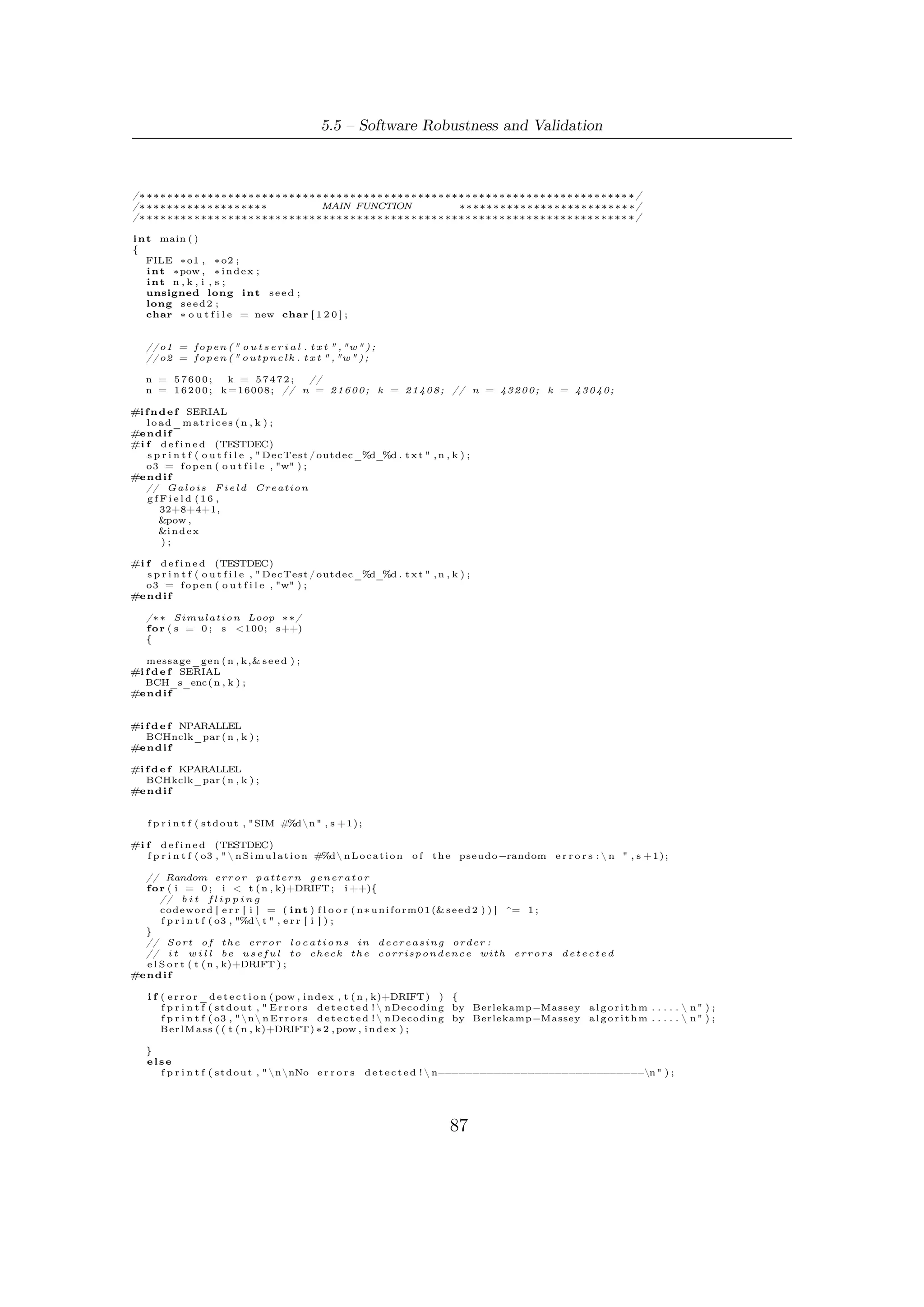
100. 6.1 – Introduction
Our goal has been to carry out a parallel bit interleaving by means of a block
that outputs one modulation signal per clock cycle in order to maximize the
achievable baud rate. In this case, if fck [MHz] is the operating frequency, we
will have a maximum achievable baud rate equal to fck [MBaud].
The goal is obtained by means of a parallel architecture, which allows to read
η consecutive bits per clock cycle belonging to different symbols; in this way,
we provide one symbol per clock cycle.
Mapper Block Mapping into constellation is carried out according to the selected
modulation format (Q-PSK or 8-PSK); constellations are stored in a ROM
(Read Only Memory) and a 7-bit representation has been used for I and Q
components.
Shaping Filter The I and Q data paths at the output of the serial to parallel block
are processed by the SRRC (Squared Root Raised Cosine) filter and polyphase
interpolator included on the same structure.
This filter is used to provide the interpolation and pulse shaping of the data in
order to minimize intersymbol interference. The complex valued coded symbols
stream is applied at the input of this sub-unit which performs SRRC pulse
shaping by a FIR filter running at rate 3Rs . The choice of a processing rate
equal to 3Rs is made considering that the desired sampling frequency fSA is
achieved by interpolating the shaped signal; as a consequence an adequate
attenuation of the signal spectrum replica, centered around the interpolator
input sampling frequency, is required.
Interpolator Section In this specific case a third order Farrow Interpolator block
has been used to change the rate at the output of the polyphase filter, depending
on the input bit rate selected.
Digital Up Conversion (UPC) Stage This block realizes the up-conversion from
the baseband frequency to the intermediate frequency.
DAC Precompensation Filter This block has been designed to compensate the
signal distortion (about 4 dB from DC to half the sampling frequency) intro-
duced by the D/A conversion; in order to correct this linear distortion a FIR
filter is used, just before the DAC.
This is most for a number of reasons, e.g. the need for complex filter coefficients
in case compensation were done at base-band; however, high speed operations
are actually desirable: hence, a coefficient simplification is introduced to avoid
multiplications and the transpose form of a FIR filter has been used; pipelining
can also be used for it to further enhance speed if required.
91

101. 6 – Preliminary Laboratory Test of DVB-S2 TX Section
Figure 6.1: TX Section Architecture
92

102. 6.2 – Test Objectives and Setup
6.2 Test Objectives and Setup
Aim of this test campaign is to verify the encoder and modulator design and its
performances in terms of constellation implementation quality: this is pursued via a
statistical characterization on phase and magnitude error.
All tests have been performed after synthesizing the VHDL-based design onto a
Stratix II DSP Development Board, which includes an EP2S180 device. Additionally,
this board provides two 14-bit D/A converters with an up to 165-Megasample per
second rate and single-ended output.
In order to best evaluate the modulator performances, signal at the output of
D/A converter has been routed to an ultra-broadband Vector Signal Analyzer (VSA)
which also executes demodulation. The VSA is composed by the association of:
1. a MSO6054A 6000 series oscilloscope (500 MHz bandwidth, 4 Gsa/s);
2. the 89601A vector signal analyzer software, running onto a PC interconnected
to the oscilloscope via an Ethernet port.
Test setup equipments is shown in Figure 6.2, Stratix II FPGA hosts the VHDL-
based design.
Figure 6.2: Laboratory Test
In particular, sampling rate and IF center frequency have been designed in order
to meet the requirements in presence of the HW constraints imposed by both the
prototyping board and the anti-image filters available. A parallel to serial converter
at the output of modulator has been added to serialize the four parallel data streams
at the output of Tx section. Note that the four parallel flows are normally necessary
to relax the high speed as well as the relevant criticality in the transfer of data from
the TX DSP section to the DAC. The overall transmitter schematic diagram is shown
in figure above.
93

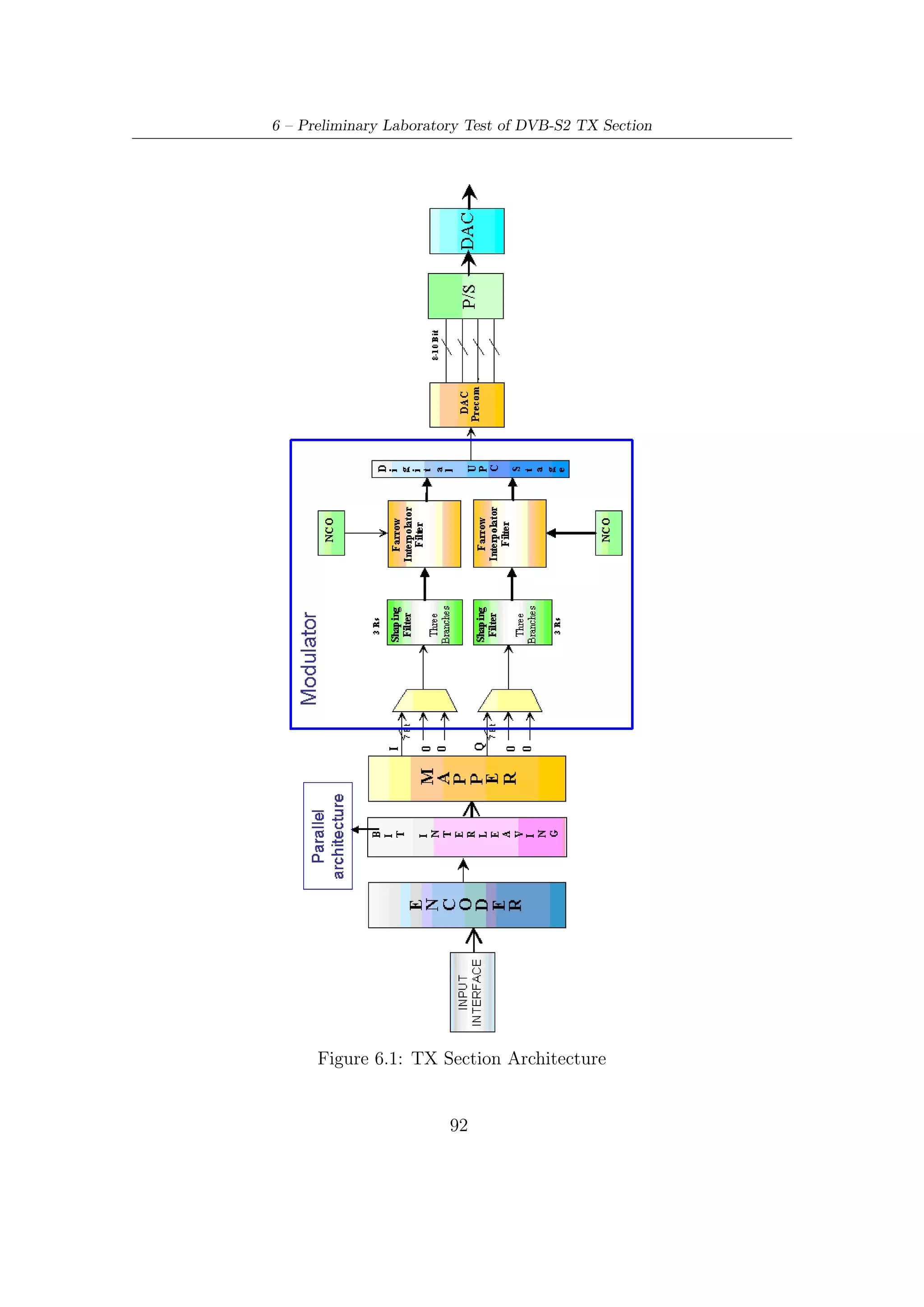
103. 6 – Preliminary Laboratory Test of DVB-S2 TX Section
Tx section performances have been evaluated in terms of constellation quality,
furthermore, a statistical analysis of magnitude and phase errors has been computed
exploiting the dedicated tool available in VSA.
The tool is based on the EVM (Error Vector Magnitude) analysis. EVM is
the Root Mean Square (RMS) of the error vectors computed and expressed as a
percentage of the square root of the mean power of the ideal signal. The instrument,
apart from peak values, can also provide the statistically estimated standard deviation
of the EVM and of the phase error.
The error vector is the magnitude of the vector, at the detected symbol location,
which connects the I/Q reference-signal phasor to the I/Q measured-signal phasor,
and is computed as follows (for a graphical representation refer to the phasor diagram
shown below):
EVM[n] = Ierr [n]2 + Qerr [n]2 (6.1)
where the variable n indicates the discrete symbol time and obviously the error in
phase is Ierr = IRef − IMeas , that is, the reference I component is subtracted to the
measured component. In a similar way the component of error in quadrature can be
measured as follow: Qerr = QRef − QMeas .
Figure 6.3: Error vector magnitude computation
In addition, magnitude error and phase error (computed as described in Figure
6.4) vs time diagram (expressed in symbols) have been plotted to better evaluate
constellation quality.
94

104. 6.2 – Test Objectives and Setup
Figure 6.4: Magnitude and phase error computation
95

105. 6 – Preliminary Laboratory Test of DVB-S2 TX Section
6.3 Test Results
In this preliminary test campaign, some measurements on the developed DVB-S2
TX section have been performed. For both 2 MBaud and 30 MBaud symbol rates,
demodulated signal constellations have been plotted.
From a statistical point of view, modulator performance have been evaluated
computing phase and magnitude error in the way indicated before.
From results of these preliminary test, degradation due to imperfect image
rejection and DAC distortion is clear.
6.3.1 2 MBaud — 16 APSK
In this test, signal constellation demodulated by VSA has been visually and quali-
tatively analyzed. In addition, phase and magnitude error have been plotted and
quantified via statistical measurements to better analyze the modulation quality.
Figure 6.5: 2MBaud 16 APSK constellation
The statistical analysis of errors leads to the following results:
96

106. 6.3 – Test Results
EVM 2%
Magnitude Error 0,9%
Phase Error 3 deg
A very limited degradation with respect to the ideal constellation is actually evident.
(a) Signal Spectrum (b) Replica Distance
Figure 6.6: 2 MBaud 16-APSK Signal spectra
97

107. 6 – Preliminary Laboratory Test of DVB-S2 TX Section
6.3.2 30 MBaud — 8 PSK
In this test, degradation of modulator performances due to the absence of a DAC
pre-compensation filter is clear. In following figures a less scattered plot with
pre-compensation filter can be seen.
(a) Signal constellation quality in presence (b) Signal constellation quality in absence
of DAC compensation of DAC compensation
Figure 6.7: 30 MBaud 8-PSK Scatter Plots
Signal spectra comparison in Figure 6.8 shows the distortion introduced by
the DAC: the blue curve, as a matter of fact, is the no-precompensated signal
spectrum, which results in a very scattered constellation (Figure 6.7b); the yellow one,
representing the signal spectrum of the same signal processed by the precompensation
filter, results in a better scatter plot.
The statistical analysis of errors leads to the following results:
Without pre-compensation With pre-compensation
filter filter
EVM 9% 4%
Magnitude Error 6% 2%
Phase Error 3 deg 1,5 deg
98

108. 6.3 – Test Results
Figure 6.8: Spectra comparison between the spectrum of the signal precompensated
(yellow one) and that of the signal non-precompensated (blue one)
99

109. 6 – Preliminary Laboratory Test of DVB-S2 TX Section
6.3.3 30 MBaud — 16 APSK
In this test, signal constellation demodulated by VSA has been visually and quali-
tatively analyzed. In addition, phase and magnitude error have been plotted and
quantified via statistical measurements to better analyze the modulation quality.
(a) Scatter (b) Scatter
Figure 6.9: 30 MBaud 16-APSK Scatter Plots
The statistical analysis of errors leads to the following results:
EVM 3%
Magnitude Error 1,5%
Phase Error 2 deg
100

110. 6.4 – 64-APSK Modulator
6.4 64-APSK Modulator
The modulator tested by TAS can also provide modulations of higher order with
respect to DVB-S2 (e.g. MHOMS modulation schemes). Figure shows a progressive
expansion of time-scale representation for a 64-APSK modulation scheme, being this
the most innovative modulation, and the four signal envelope level either(points lie
on 4 concentric circumferences, that is, each radius represents the amplitude of each
level provided).
(a) (b)
(c) (d)
Figure 6.10: 64-APSK Signal
101

111. 6 – Preliminary Laboratory Test of DVB-S2 TX Section
102

112. Chapter 7
Conclusions
In this thesis we have dealt with a digital communications TX section which can
provide a reliable information transmission via satellite while complying with the
challenging requirements on performance imposed by DVB-S2 standard.
My most working contributions to the overall project of the DVB-S2 TX section
developed by TAS-I have been focused specifically on
• study of the theory underlying the BCH code: Galois fields and cyclic codes
theory in order to have the theoretical basis to understand the DVB-S2 code
structure and analyze algorithms related to;
• theoretical analysis of DVB-S2 BCH code structure from which we have reach
the conclusion that the DVB-S2 outer code (BCH) must be primitive and
shortened ;
• study of the BCH encoding procedures and algorithms and its related (serial)
architectures;
• modelling and design of a parallel BCH encoder with a high degree of parallelism
in order to best match the TX Section (developed by TAS) speed requirements;
• development of a Berlekamp-Massey software decoder in order give a proof
of the error correction capacity of the code (encoder); to this purpose we
have defined specifical routines aimed to compute arithmetic tables useful in
decoding and error detection computations;
• development of a software package (C/C++) in order to verify the functioning
of architectures envisaged and give support to VLSI designers in validation of
the correspondent VHDL model;
103

113. 7 – Conclusions
Concerning to the DVB-S2 architecture and overall TX section and thanks to
the contribution of the TAS-I Algorithm & Architectures team, this thesis has dealt
with:
• identification of the strategic importance of satellite communications in some
application scenarios such as Multimedia, Earth observation, radio-localization
and navigation, etc.;
• review of novel techniques aimed at obtaining top performance by handling
modulation and coding schemes jointly;
• assessment of the features of ACM techniques, which allow to better utilization
of resources onboard while ensuring a high QoS (Quality of Service);
• design of the DVB-S2 Modem architecture and blocks focusing on concatenated
coding (BCH-LDPC) and modulation schemes;
• qualitative description of LDPC encoding/decoding algorithms, and on the
latter we have highlighted the importance of the BCH code to counteract
against error floors affecting LDPC iterative decodings;
• BCH encoding procedures and algorithms and its related (serial) architectures;
• modelling and design of a parallel encoder with a high degree of parallelism in
order to best match the TX Section (developed by TAS-I) speed requirements;
• selection between two possible (and functionally equivalent) BCH parallel
architectures in order to work in ACM;
• development of a Berlekamp-Massey software decoder in order give a proof
of the error correction capacity of the code (encoder); to this purpose we
have defined specifical routines aimed to compute arithmetic tables useful in
decoding and error detection computations;
• development of a software package (C/C++) in order to verify the functioning
of architectures envisaged and give support to VLSI designers in validation of
the correspondent VHDL model;
• participation to a preliminary laboratory test and validation of the TAS-I
developed DVB-S2 TX section .
104

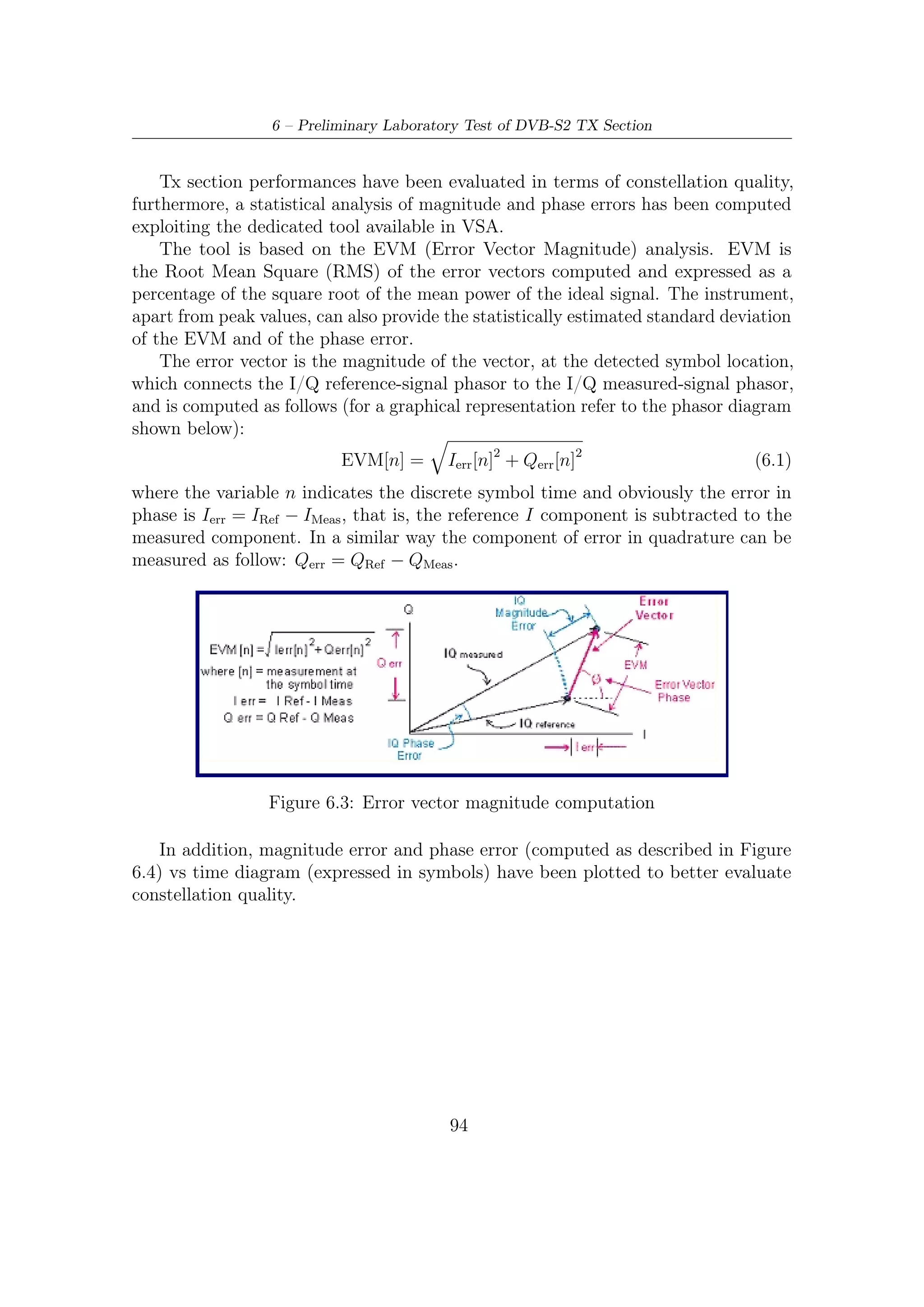
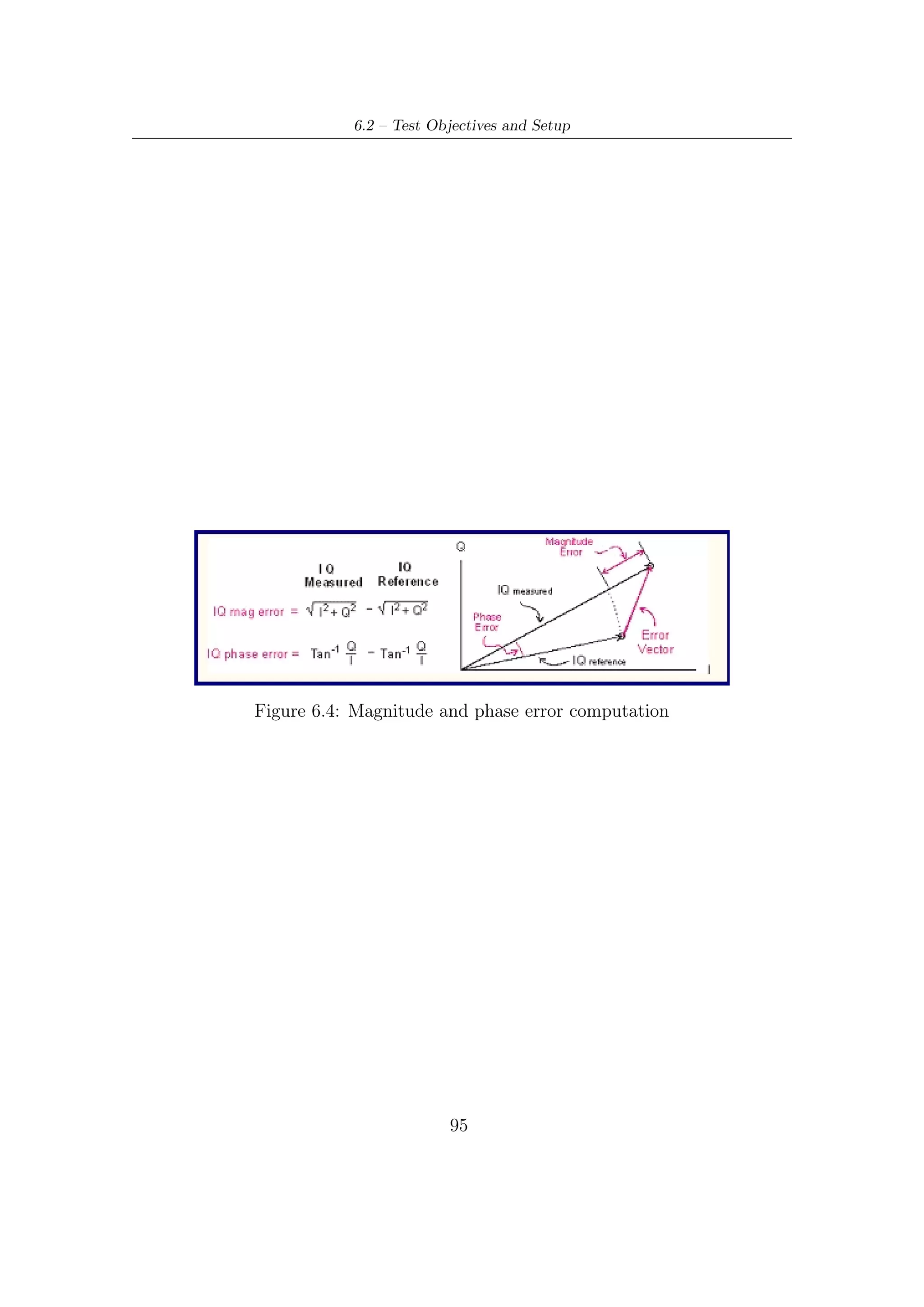
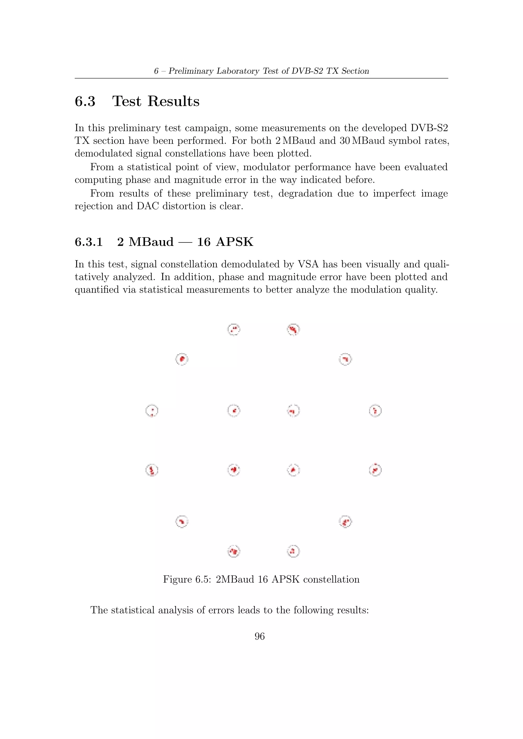
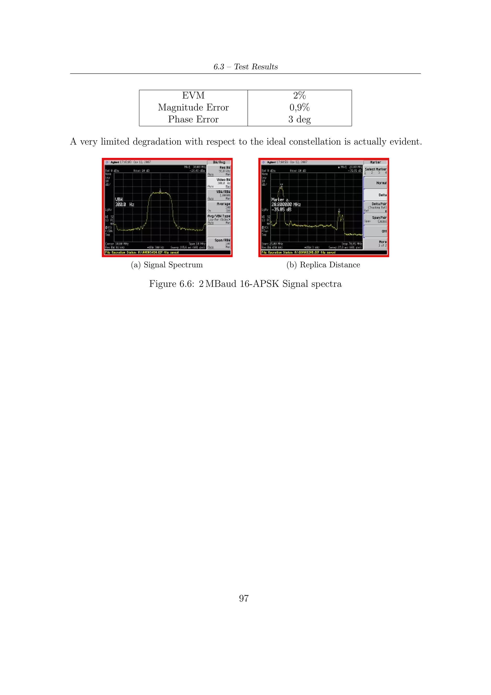
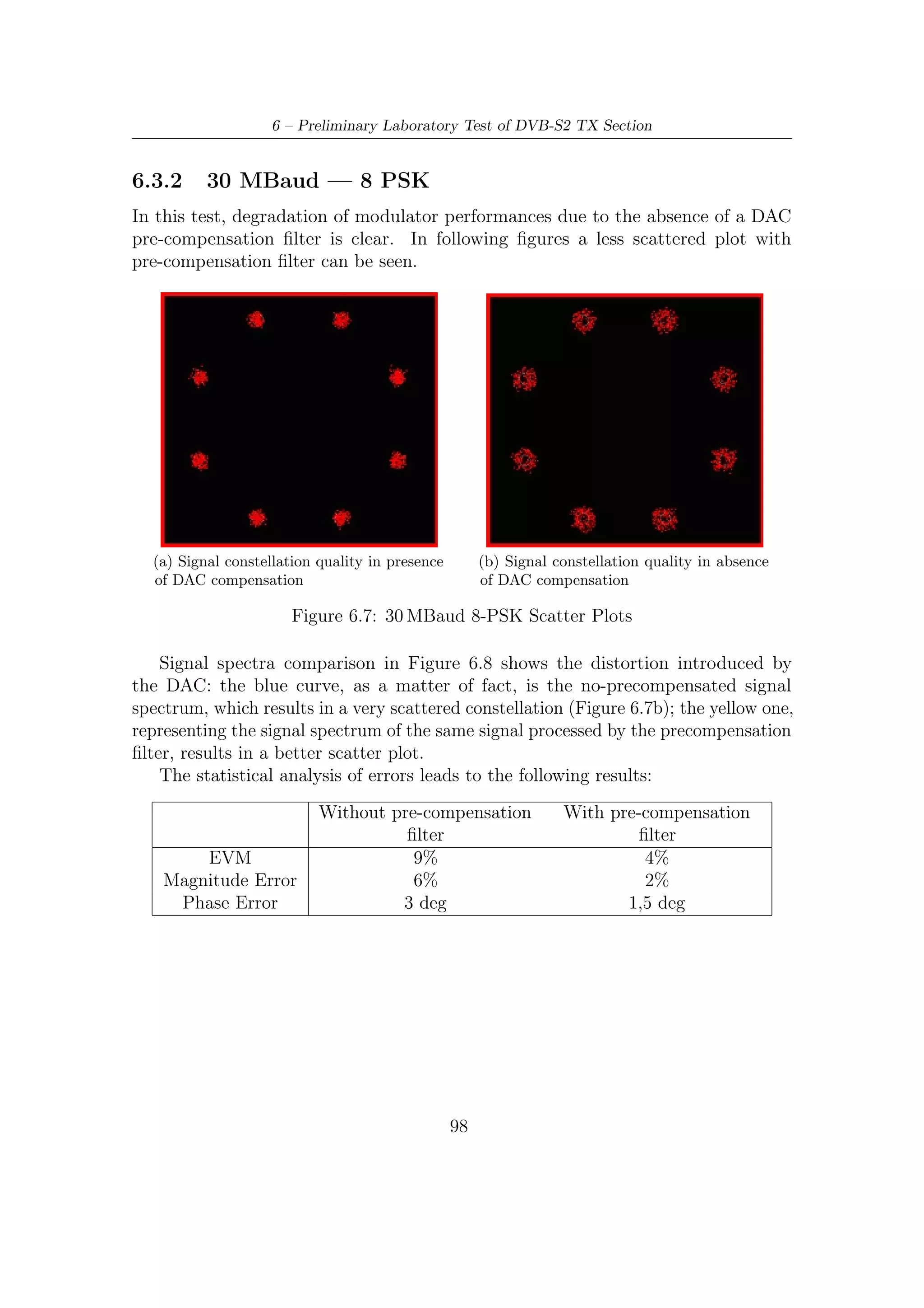
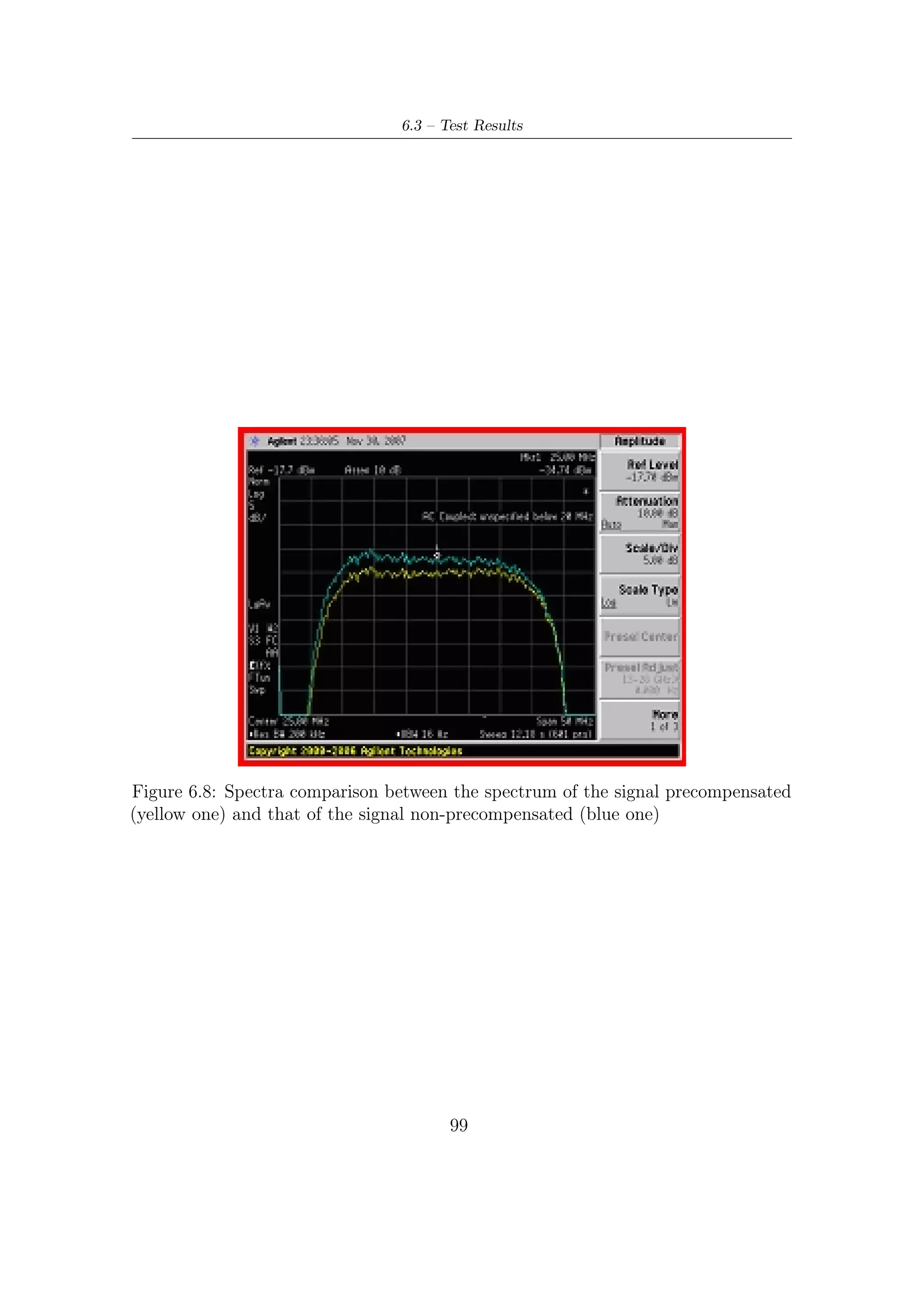
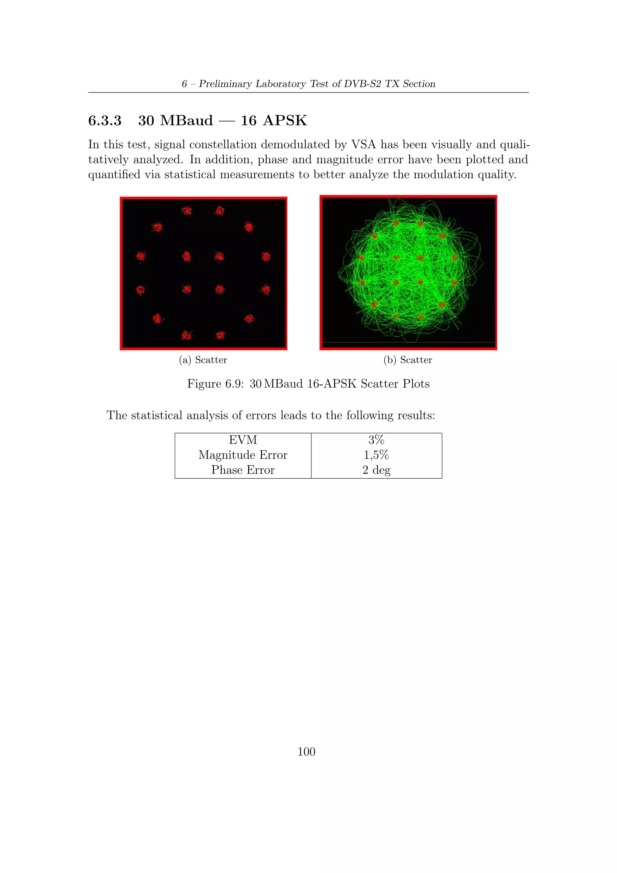
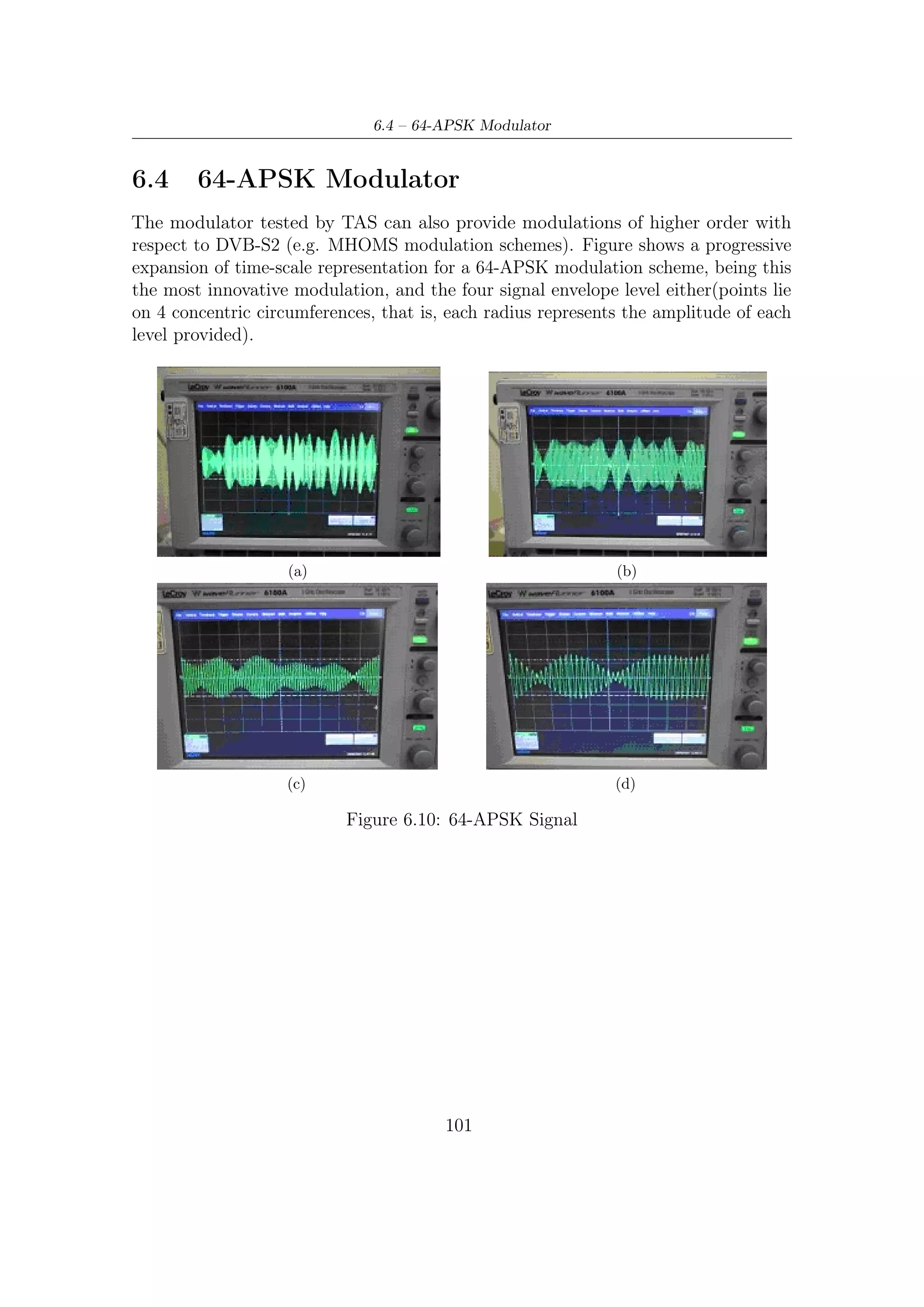
114. Appendix A
Galois (or Finite) Fields
In this appendix we introduce some basic coding concepts related to error correction
coding with a particular focus on mathematical tools come in useful through DVB-
S2 FEC encoding. Obviously, we do not provide a complete treatment of such a
rigorous and abstract mathematical theory. First, because it not so worth for our
purposes; second, because there are several books written over Coding Theory where
is exhaustively and rigorously explained all that could be necessary. Therefore, for
any further information over the next presented topics, the reader could refer, for
example, to [15] or [9].
In engineering application it is often necessary finding a reasonable trade-off
between system complexity and performance achieved. On the one hand, elementary
decoding approach is simpler, but, on the other hand, its computational burden
increases exponentially with the length of code. Algebraic decoding represents a
valid alternative to overcome such a huge complexity grow.
The key idea concerning the algebraic coding is that of giving codes some
algebraic structure to be exploited for decoding purposes. When length of block
become rather great decoding turn out to be somewhat intractable. For example,
the hard decision on the minimum distance between received sequence and codeword
requires a computational effort and a big amount of memory, both increasing with
the length of code. An other approach is the standard array decoding. Unfortunately,
this also turns out to be too expensive when the block dimensions become large. In
particular, its memory requirements make this approach rather unattractive.
Algebraic coding/decoding is based on a large extent of powerful and elegant
algebraic structures called finite fields. A field is essentially a set of elements where
addition, subtraction, multiplication and division operations yield always an element
within such set. A well known example of a field is R, the infinite field of real
numbers. Although the following observation could be rather trivial, the need of such
an algebraic structure is straightforward. Finite fields act as the most common real
fields. The unique difference is that the size of the set is finite as, for example, an
105

115. A – Galois (or Finite) Fields
ensemble of codewords. Note, for example, that any codeword could not be decoded
by Berlekamp-Massey algorithm or Galois Field Transform if inverse property was
not satisfied.
Although the preliminary concepts over axioms and elementary algebraic struc-
tures which lead to rigorous mathematical definition of field properties are even
important, the real core of this appendix is the part as to factorization of a ‘special
polynomial’. This operation provides, together with some elementary knowledge on
the Coding Theory, a powerful tool to design and well understand algebraic encoding
and decoding algorithms.
A.1 Algebraic Structures: a Glance
Before discussing properties of finite fields, let us define some preliminary algebraic
structures. Let us start from the definition of groups. On this sets it is possible
to define some (binary) operations between their elements. To be called a group,
operations over such a set must satisfy these following algebraic properties.
Definition A.1.1. A binary operation ∗ on a set assigns to each ordered pair of
elements of the set (a, b) some element of the set. (This is defined as closed binary
operation.)
Definition A.1.2. A group is a set G, + together with a binary operation ∗ on G
such that:
G1 The operator is associative: for any a, b, c ∈ G, (a ∗ b) ∗ c = a ∗ (b ∗ c).
G2 There is an element e ∈ G called the identity element such that a ∗ e = e ∗ a
for all a ∈ G.
G3 For every a ∈ G, there is an element b ∈ G known as the inverse of a such that
a ∗ b = e The inverse of a is sometimes denotes as a−1 (when the operator ∗ is
multiplication-like) or as −a (when the operator ∗ is addition-like).
G4 If also a ∗ b is equal to b ∗ a, the group is also an abelian (or commutative)
group.
If the commutative property holds then a group is said abelian. It is possible to
define an algebraic structure as a group also on a finite set of elements, as well as on
those infinite.
Definition A.1.3. If G has a finite number of elements, it is said to be a finite
group. Furthermore, such number is called the order (or the cardinality) of the
group.
106

116. A.2 – How Do We Get Galois Fields?
Let Zn , + denote addition on the numbers {0, 1, . . . , n − 1} modulo n. Clearly
such set is an abelian group, since, as it is shown in explicative Table A.2 (which can
be easily generalized) 0 is the identity element appearing in each column; moreover,
the uniqueness of solution proves associative property; furthermore, the addition
table or its generalization is symmetric and thus the operation is commutative.
Let us now introduce another algebraic structure, the ring, which will be later
helpful in the examination of cyclic codes. Differently from groups, rings have two
binary operation associated with them.
Definition A.1.4. A ring (loosely speaking) is a set where addition, subtraction
and multiplication are possible. Formally, R is an additive abelian group, together
with a multiplication satisfying ab = ba, a(b + c) = ab + ac, (ab)c = a(bc), and which
contains an identity element 1 such that 1 · a = a.
As also shown in Table A.2, the multiplication under Zn does not form a group:
there is a presence of zeros in correspondence of columns which denote the nonzero
elements (see the next section for the zero divisor formal definition). In fact, in a
ring, not every element has a multiplicative inverse, whereas, in a field, the familiar
arithmetic operations that take place in the usual real numbers are all available.
Definition A.1.5. A field is a set of objects F on which the operations of addition
and multiplication, subtraction (or additive inverse), and division (or multiplicative
inverse) apply in a manner analogous to the way these operation work for real
numbers. That is
F1 The elements of F form an abelian (or commutative) group under addition.
F2 The non-zero elements of F form an abelian group under multiplication.
+ 0 1 2 3 4
0 0 1 2 3 4
1 1 2 3 4 0
2 2 3 4 0 1
3 3 4 0 1 2
4 4 0 1 2 3
Table A.1: Addition table under Z5
A.2 How Do We Get Galois Fields?
Let us now try to find a relationship between groups and fields. More specifically,
starting from the rings with addition and multiplication operations modulo n, we
107

117. A – Galois (or Finite) Fields
· 0 1 2 3 4 5
0 0 0 0 0 0 0
1 0 1 2 3 4 5
2 0 2 4 0 2 4
3 0 3 0 3 0 3
4 0 4 2 0 4 2
5 0 5 4 3 2 1
Table A.2: Multiplication table under Z6
wish to comprehend how obtaining a finite field and under which hypothesis. To this
purpose, it could be interesting to note that, in some cases, each nonzero element of
a ring has a multiplicative inverse and so is a field, while, in other ones, there exist
some elements without a multiplicative inverse. We could start to observe that when
the ring characteristic is a prime number (as five, see Table A.3), we have a ring
with elements forming an abelian group under multiplications. The reasons will be
made more clear after this following definition as to elements called as zero divisors.
Definition A.2.1. In a ring R, if a, b ∈ R with both a and b not equal to zero but
ab = 0, then a and b are said to be zero divisors.
In practice, the presence of zero divisors make a ring impossible to have a
multiplicative inverse for each its elements and, above all, have a multiplicative
structure closed under multiplicative operations.Therefore, if we have no zero divisors
then a finite ring is also a Galois (or finite) field. The following theorem defines
under which hypothesis no such elements exist.
Theorem A.2.1 (Todd K. Moon, [15]). The ring Zp is a field if and only if p is a
prime.
Without making any mathematical calculations, we can observe (as proof) that
if p is a prime its multiples over Zp cannot exist and, therefore, neither zero divisors.
Besides the finite fields with p prime, there are other finite fields. As the field
of complex numbers C can be constructed as a field extension from the field of real
numbers R, these Galois fields are extension fields of Zp . More in detail, extension
fields are constructed to create roots of irreducible polynomials that do not have
roots in base fields. E.g., the polynomial f (x) = x2 + 1 is irreducible over R, but not
over C where we can write:
f (x) = (x + α)(x − α) = (x + j)(x − j) (A.1)
Practically we obtain an extension field from a base field whenever we can find any
irreducible polynomial over the base field. Loosely speaking, these polynomials may
be conceived as prime numbers by which (as noticed previously) it is possible to
construct any fields.
108

118. A.3 – A Mathematical Survey
· 0 1 2 3 4
0 0 0 0 0 0
1 0 1 2 3 4
2 0 2 4 1 3
3 0 3 1 4 2
4 0 4 3 2 1
Table A.3: Multiplication table under Z5
A.3 A Mathematical Survey
Having shown how to obtain Galois fields, we now lay out some aspects of the theory.
We first focus on the additive structure of finite fields, which tells us what size any
finite fields can be. Recalling Theorem A.2.1, it follows that there are p elements
which behave as a field (i.e., we can define addition and multiplication on them as a
field). Thus, Zp is a subfield of every Galois fields GF (q). In fact, an assertion can
be made:
Theorem A.3.1 (Todd K. Moon, [15]). The order q of every finite fields GF (q)
must be a power of a prime.
By Theorem A.2.1, every finite fields GF (q) has a subfield of prime order p. In
fact, it can be shown that GF (q) acts like a vector space over its subfield GF (p).
More specifically, if we get
a1 β1 + a2 β2 + . . . + am βm (A.2)
with coefficients ai lying over GF (p) and βi ∈ GF (q = pm ) we can obtain all
the distinct elements of GF (q). In other words, each combination of coefficients
{a1 , a2 , · · · , am } corresponds to a distinct element of GF (q).
This theorem shows that all finite fields have the structure of a vector space of
dimension m over a finite field Zp . For the field GF (pm ), the subfield GF (p) is called
the ground field.
By definition, each element of a finite field forms a group under multiplication.
Let us now try to understand how they behave, giving at the same time some helpful
definitions.
1
Definition A.3.1. Let β ∈ GF (q). The order of β, written ord(β) is the smallest
positive integer such that β n = 1.
Definition A.3.2. An element with order q − 1 in GF (q) (i.e, it generates all the
nonzero elements of the field) is called primitive element.
1
The nomenclature is slightly misguiding, since we already defined the order of a group.
109

119. A – Galois (or Finite) Fields
In other words, a primitive element has the highest possible order. Since every
elements of the field are representable by that, this ‘special element’ (or elements)
enables the ‘power representation’ of the field, which much simplify multiplication.
In the brackets of this last sentence we have referred to a more than one possible
existence of these primitive elements. More specifically, they are φ(q − 1) (i.e., Euler
totient function [15]), as following theorem asserts.
Theorem A.3.2 (Todd K. Moon, [15]). There are φ(q − 1) primitive elements in
GF (q).
If α ∈ GF (q) is primitive, then
{α, α2 , . . . , αq−2 , αq−1 = 1}
is the set of nonzero elements of GF (q). But, if β = αi is also primitive then the
nonzero elements of the fields are still generated by
{β, β 2 , . . . , β q−2 , β q−1 = 1}
Although these are different generators, these are not different fields, but only different
representations.
Since, as we previously said, every field element can be written as β = αi ∈ GF (q)
we have the following.
Theorem A.3.3 (Todd K. Moon, [15]). Every element of the field GF (q) satisfies
the equation xq − x = 0. Furthermore, they constitute the entire set of roots of this
equation.
Its proof is trivial: let α a primitive element. Then imposing β = αi yields
q−1 i
(αi ) = (αq−1 ) = 1 which satisfies the equivalent equation xq−1 − 1 = 0.
A.4 Irreducible and Primitive polynomials
While any irreducible polynomial can be used to construct the extension field,
computation in the field is easier if a primitive polynomial is used. We make the
following observation:
Theorem A.4.1 (Todd K. Moon, [15]). Let p a prime. An irreducible mth-degree
m
polynomial f (x) ∈ GF (p)[x] divides xp −1 − 1.
Let GF (q) = GF (pm ) be constructed using the irreducible polynomial f (x),
where α denotes the root of f (x) in the field: f (α) = 0. By Theorem A.3.3, α is a
m
root of xp −1 − 1 in GF (q). Using the division algorithm (i.e., Euclid theorem) write
m −1
xp − 1 = g(x)f (x) + r(x) (A.3)
110

120. A.5 – Factoring xn − 1
where deg(r(x)) ≤ m. Evaluating above equation at x = α we obtain
0 = 0 + r(α)
But the elements of the field GF (q) are represented as polynomials in α of degree
less equal to m, so since r(α) = 0 it must be that r(x) is a zero polynomial, r(x) = 0.
Definition A.4.1. An irreducible polynomial p(x) ∈ GF (p)[x] of degree m is said
to be primitive if the smallest positive integer n for which p(x) divides xn − 1 is
n = pm − 1.
Theorem A.4.2 (Todd K. Moon, [15]). The roots of an mth degree primitive
polynomial p(x) ∈ GF (p)[x] are primitive elements in GF (pm )
In other words, any of the roots can be used to generate the nonzero elements of
the field GF (pm ). Furthermore, all the nonzero elements of the field can be generated
as power of the roots of the primitive polynomial.
A.5 Factoring xn − 1
To design and understand cyclic codes, it is worth succeeding in factorization of
xn − 1 over arbitrary finite fields.
m
From Theorem A.3.3, we know that every element of GF (q m ) is a root of xq −1 −1,
so m q −1
m −1
xq −1= (x − αi )
i=0
m
for a primitive element α ∈ GF (q ). To provide a factorization over the field GF (q)
, the factors x − αi can be grouped together according to conjugacy classes. First of
all, let us describe some concepts related to.
Definition A.5.1. Let β ∈ GF (q m ). The conjugates of β with respect to a subfield
2 3
GF (q) are β, β q , β q , β q , .....
Since the field is finite, the above list must repeat at some point. This is provided
by the following.
Definition A.5.2. The smallest positive integer d such that n is divisible by q d − 1
is called multiplicative order of q modulo n.
Furthermore, if any β ∈ GF (q m ) have ord(β) = n and d multiplicative order of
d 2 d−1
q modulo n, then β q = β. The d elements β, β q , β q , . . . , β q are all distinct. In
addition, it can be proved the following.
111

121. A – Galois (or Finite) Fields
Theorem A.5.1 (Todd K. Moon, [15]). Let β ∈ GF (q m ) have order n and let
d be the multiplicative order of q mod n. Then the coefficients of the polynomial
p(x) = d−1 (x − β q ) are in GF (q). Furthermore, p(x) is irreducible. That is, p(x)
i
i=0
is the minimal polynomial for β.
Conjugacy Class Minimal Polynomial
{0} x
{1} x+1
{α, α2 , α4 } (x − α)(x − α2 )(x − α4 ) = x3 + x + 1
{α3 , α6 , α5 } (x − α3 )(x − α6 )(x − α5 ) = x3 + x2 + 1
Table A.4: Conjugacy Classes over GF (23 ) with respect to GF (2)
Conjugacy Class Minimal Polynomial
{0} x
{1} x+1
{α, α2 , α4 , α8 } (x − α)(x − α2 )(x − α4 )(x − α8 ) = x4 + x + 1
{α3 , α6 , α9 , α12 } (x − α3 )(x − α6 )(x − α9 )(x − α12 ) = x4 + x3 + x2 + x + 1
{α5 , α10 } (x − α5 )(x − α10 ) = x2 + x + 1
{α7 , α11 , α13 , α14 } (x − α7 )(x − α11 )(x − α13 )(x − α14 ) = x4 + x3 + 1
Table A.5: Conjugacy Classes over GF (24 ) with respect to GF (2)
m
We now are ready to understand that xq −1 − 1 can be expressed as a product
of the minimal polynomials of the nonzero elements. For example the polynomial
3
x7 −1 = x2 −1 −1 can be factored over GF (2) as a product of the minimal polynomials
shown in Table A.4
x7 − 1 = (x + 1)(x3 + x + 1)(x3 + x2 + 1) (A.4)
To generalize problem of factoring xn − 1 when n = q m − 1, let any element β = 1
/ /
such that β = 1 call a nth root of unity. First, we have to determine a field GF (q m )
n
where nth root of unity can exist. Once found, factorization is accomplished using
the minimal polynomials in such field.
Since there are φ(n) elements of order n in GF (q m ), finding a field GF (q m ) with
n roots of unity requires finding an m such that n|q m − 1 (i.e, n must be a divisor of
q m − 1). This is usually done by trial and error.
Once any β of order n is found, then beta is a root of xn − 1 in that field, and so
are the elements β 2 , β 3 , . . . , β n−1 . In other words,
n−1
n
x −1= x − βi (A.5)
i=0
112

122. A.5 – Factoring xn − 1
For example, let now determine an extension field GF (2m ) in which 5th roots of
unity exist and express the factorization in term of polynomials in GF (2)[x]. Since 5
is the smallest divisors of 24 − 1, the roots of unity are over GF (16). So if we let
β = α3 , α primitive, then β 5 = α1 5 = 1. Thus the roots of x5 − 1 = x5 + 1 in GF (16)
are
1, β, β 2 , β 3 , β 4
which can be expressed in terms of the primitive element α as
1, α3 , α6 , α9 , α12
Using the minimal polynomials shown in Table A.5 we have
x5 − 1 = (x + 1)(x4 + x3 + x2 + x + 1)
113

123. A – Galois (or Finite) Fields
114

124. Appendix B
Cyclic Codes
We now deal with cyclic codes, which have additional algebraic structure to make
encoding and decoding more efficient. In other words, they have some structure that
can be easily exploited through encoding/decoding stages. Note that one of the most
notorious cyclic codes are the Hamming codes. In fact, from a certain point of view,
BCH codes can be conceived as an extension of Hamming codes. This ‘parallelism’
is well shown in [21], [9].
Cyclic codes are based on polynomial operations. A natural algebraic settings
for the operation on polynomials is the algebraic structure of a ring. This appendix
presents some elementary concepts related to shift operations and linear block codes,
focusing on the algebraic description of cyclic codes. Galois fields and cyclic codes
theory together are exploited in the design of a cyclic code with a specified minimum
distance. The theoretical and practical connection between algebraic structures and
code description shows a way of reducing the computational burden in decoding.
B.1 Shift Operation
We now introduce the mathematical definition of cyclic block codes.
Definition B.1.1. A (n, k) block code C is said to be cyclic if it is linear and if for
every codeword c = (c0 , c1 , . . . , cn−1 ) in C, its right cyclic shift c = (cn−1 , c0 , . . . , cn−2 )
is also in C.
The operations of shifting and cyclic shifting can be conveniently represented
using polynomials. The vector
c = (c0 , c1 , . . . , cn−1 ) (B.1)
is represented by the polynomial
c(x) = c0 + c1 x + . . . + cn−1 xn−1 (B.2)
115

125. B – Cyclic Codes
using the obvious one-to-one correspondence. A (noncyclic) shift can be represented
by polynomial multiplication:
xc(x) = c0 x + c1 x2 + . . . + cn−1 xn (B.3)
However, if c(x) was a hypothetic codeword, the above operation obviously would
not yield any codeword.
As described in Appendix A, taking the remainder after division by xn − 1
translates into imposing xn = 1. So that getting xc(x) module xn − 1 yields
xc(x) = cn−1 + c0 x + c1 x2 + . . . + cn−2 xn−1 (B.4)
Could this result be any codeword, or rather, any element of the same set? In other
words, this point is that mathematicians call closure under a given operation (or
operator). Before dealing with this, we need to introduce another algebraic structure,
the ideals. It will show that every cyclic codes forms ideals in a ring of polynomials.
B.2 Rings of Polynomials and Ideals in Rings
Let R be a ring. A polynomial f (x) of degree n with coefficients in R is
n
f (x) = ai x i (B.5)
i=0
where an = 0. The symbol x is said an indeterminate.
/
Definition B.2.1. The set of all polynomials with an indeterminate x with coeffi-
cients in a ring R, using the usual operations for polynomial addition and multiplica-
tion, forms a ring called the polynomial ring. It is denoted as R[x].
Generally, polynomial multiplication has not an inverse. For example in the ring
of polynomials with real coefficients R[x], there is no polynomial solutions f (x) to
f (x)(x2 + 5x + 1) = x3 + 3x + 1
Let us now consider the residue class of polynomials rings GF (p)[x] modulo
xn − 1, denoted as GF (p)[x]/(xn − 1). We have already shown (A.2) that a quotient
ring is a field if and only if xn − 1 cannot be factored over the base field GF (p) (p is
a prime number). But let us return to our main question. In fact, we would like to
find a set where every its shifted elements is still within such set. Such an algebraic
structure is the following.
Definition B.2.2. Let R be a ring. A nonempty subset I ⊆ R is an ideal if satisfies
the following conditions:
116

126. B.3 – Algebraic Description
1. I forms a group under the addition operation in R.
2. For any a ∈ I and any r ∈ R, ar ∈ I.
It seems that a cyclic code form an ideal in a ring of polynomials. Furthermore,
for cyclic codes the ideals are principal, as defined by the following.
Definition B.2.3. An ideal I in a ring R is said to be principal if there exist some
g ∈ I such that every element a ∈ I can be expressed as a product a = mg for some
m ∈ R.For a principal ideal, such an element g is called the generator element. The
ideal generated by g is denoted as g :
g = {hg : h ∈ R}
Theorem B.2.1 (Todd K. Moon, [15]). Let I be an ideal in Fq /(xn − 1). Then
1. There is a unique monic polynomial g(x) ∈ I of minimal degree.
2. I is principal with generator g(x).
3. g(x) divides (xn − 1) in Fq [x].
For example, it can be shown that in GF (2)[x]
x7 − 1 = (x + 1)(x3 + x + 1)(x3 + x2 + 1)
In the ring GF (2)[x]/(x7 − 1), there are ideals corresponding to the different factor-
ization of x7 + 1, so there are the following nontrivial ideals
x+1 x3 + x + 1 x3 + x2 + 1
(x + 1)(x3 + x + 1) (x + 1)(x3 + x2 + 1) (x3 + x2 + 1)(x3 + x + 1)
B.3 Algebraic Description
As said in Section B.1, cyclic shifting of a polynomial c(x) is represented by xc(x)
modulo xn − 1 operation. Taking into account Theorem B.2.1 and what said as far,
we can therefore reach the following conclusions as to cyclic codes:
• A (n, k) cyclic code has a unique minimal monic polynomial
g(x) = g0 + g1 x + . . . + gn−k xn−k (B.6)
It, which is also the generator of ideal, is called the generator polynomial for the
code, and its degree represents the redundancy r = n − k of the code.
117

127. B – Cyclic Codes
• Every codeword can be expressed as a multiple of the generator
c(x) = m(x)g(x) (B.7)
Obviously, the degree of message polynomial m(x) is less than k, so the dimension
of the code is k. In other words, there are k independently selectable coefficients
in m(x).
Generalization for the systematic coding is straightforward. In fact, by Euclid
Theorem application we have
m(x)xn−k = q(x)g(x) + r(x) ⇒ m(x)xn−k − r(x) = q(x)g(x) (B.8)
and therefore if we conceive a codeword as m(x)xn−k − r(x) where r(x) represents
the remainder of m(x) after division by g(x), then we obtain an equivalent
representation of cyclic code. This is called in literature systematic form and it
has the following vector correspondence
(−d0 , −d1 , . . . , −dn−k−1 , m0 , m1 , . . . , mk−1 ) ↔ xn−k m(x) − r(x) (B.9)
Loosely speaking, this different encoding process has the unique effect of changing
one-to-one mapping between messages and correspondent codewords.
• Furthermore, the generator g(x) is a factor of xn−1 − 1 in GF (q)[x].
118

128. Bibliography
[1] A. Morello , V. Mignone . Il sistema DVB-S2 di seconda generazione per
la trasmissione via satellite a Unicast. Elettronica e Telecomunicazioni, (3),
December 2003.
[2] Claude Berrou, Alain Glavieux, Punya Thitimajshima. Near Shannon Limit
Error – Correcting Coding and Decoding: Turbo Codes. IEEE, 1993.
[3] Claude E.Shannon. A Mathematical Theory of Communications. The Bell
System Technical Journal, 27:379–423, 623–656, July, October 1948.
[4] D. Giancristofaro , M. Fonte , A. Bernardi , I. Martinazzo , M. Livi , R. Novello
, A. Ginesi , S. Benedetto , G. Montorsi , M. Luise , L. Giugno . The MHOMS
1 Gbps Modem for Future Earth Observation.
[5] David J.C. MacKay. Information Theory, Inference, and Learning Algorithms.
Cambridge University Press, 2003.
[6] European Telecommunications Standard Institute, 650 Route des Lucioles F-
06921 Sophia Antipolis Cedex - FRANCE. EN 302 307 v1.1.1 — Digital Video
Broadcasting (DVB); Second generation framing structure, channel coding and
modulation systems for Broadcasting, Interactive Services, News Gathering and
other broadband satellite applications, March 2005.
[7] European Telecommunications Standard Institute, 650 Route des Lucioles F-
06921 Sophia Antipolis Cedex - FRANCE. TR 102 376 v1.1.1 — Digital
Video Broadcasting (DVB); User guidelines for the second generation system for
Broadcasting, Interactive Services, News Gathering and other broadband satellite
applications (DVB-S2), March 2005.
[8] Ezio Biglieri. Digital Transmission in the 21st Century: Conflating Modulation
and Coding. IEEE Communications Magazine, pages 128–137, May 2002.
[9] F. J. MacWilliams, N. J. Sloane. The Theory of Error-Correcting Codes,
volume 16. North-Holland, I edition, 1977.
[10] G.Caire, G.Taricco, E.Biglieri. Bit Interleaved Coded Modulation. IEEE, pages
1463–1466, 1997. Research supported by European Space Agency (ESA).
[11] Gottfried Ungerboek. Channel Coding with Multilevel/Phase Signal. IEEE
Transactions on Information Theory, (1):55–67, January 1981.
[12] John G. Proakis. Digital Communications. McGraw-Hill, III edition, 1995.
119

129. Bibliography
[13] Joohee Kim, Russell M. Mersereau, Yucel Altunbasak. Error-Resilient Image
and Video Transmission Over the Internet Using Unequal Error Protection.
IEEE TRANSACTIONS ON IMAGE PROCESSING, 12(2):121–131, February
2003.
[14] Michael Gallant, Faouzi Kossentini. Rate-Distortion Optimized Layered Coding
with Unequal Error Protection for Robust Internet Video. IEEE TRANS-
ACTIONS ON CIRCUITS AND SYSTEMS FOR VIDEO TECHNOLOGY,
11(3):357–372, March 2001.
[15] Todd K. Moon. Error Correction Coding — Mathematical Methods and Algo-
rithms. Johnb:ACMBiglieri Wiley and Sons, Inc., 1th edition, March 2005.
[16] P.Robertson and T.Worz. Bandwidth-efficient turbo trellis-coded modulation
using punctured component codes. IEEE J. Select. Areas Commun., 16(2):206–
218, February 1998.
[17] Robert Gallagher. Low-Density Parity-Check Codes. Revisited Version, Mas-
sachussets Institute of Technology, Cambridge, Mass., July 1963.
[18] Roberto Garello, Franco Chiaraluce, Paola Pierleoni, Marco Scaloni, Sergio
Benedetto. On Error Floor and Free Distance of Turbo Codes.
[19] S. Benedetto , R. Garello , G. Montorsi , C. Berrou , C. Douillard , D. Gian-
cristofaro , A. Ginesi , L. Giugno , M. Luise . MHOMS: High Speed ACM
Modem for Satellite Application. IEEE Wireless Communications, 2005.
[20] S.Fagioli, A.Capuzi, R.Leonardi, G.Angino. COSMO-SKYMED: The Italian
Contribution to The French-Italian Inter-Governmental Agreement on Earth
Observation. Customer Application Note, 2006.
[21] Stephen B. Wicker. Error Control System for Digital Communication and
Storage. Prentice-Hall, 1995.
[22] Tom Richardson. The Renaissance of Gallager’s Low-Density Parity-Check
Codes. IEEE Communications Magazine, pages 126–131, August 2003.
120