![IEEE/ACM TRAS. ON NETWORKING, VOL. 6, NO. 1, JUNE 2008 1
Dual-resource TCP/AQM
for Processing-constrained Networks
Minsu Shin, Student Member, IEEE, Song Chong, Member, IEEE, and Injong Rhee, Senior Member, IEEE
Abstract—This paper examines congestion control issues for processing capacity in the network components. New router
TCP flows that require in-network processing on the fly in technologies such as extensible routers [3] or programmable
network elements such as gateways, proxies, firewalls and even routers [4] also need to deal with scheduling of CPU usage
routers. Applications of these flows are increasingly abundant in
the future as the Internet evolves. Since these flows require use of per packet as well as bandwidth usage per packet. Moreover,
CPUs in network elements, both bandwidth and CPU resources the standardization activities to embrace various network ap-
can be a bottleneck and thus congestion control must deal plications especially at network edges are found in [5] [6] as
with “congestion” on both of these resources. In this paper, we the name of Open Pluggable Edge Services.
show that conventional TCP/AQM schemes can significantly lose In this paper, we examine congestion control issues for
throughput and suffer harmful unfairness in this environment,
particularly when CPU cycles become more scarce (which is likely an environment where both bandwidth and CPU resources
the trend given the recent explosive growth rate of bandwidth). As can be a bottleneck. We call this environment dual-resource
a solution to this problem, we establish a notion of dual-resource environment. In the dual-resource environment, different flows
proportional fairness and propose an AQM scheme, called Dual- could have different processing demands per byte.
Resource Queue (DRQ), that can closely approximate propor- Traditionally, congestion control research has focused on
tional fairness for TCP Reno sources with in-network processing
requirements. DRQ is scalable because it does not maintain per- managing only bandwidth. However, we envision (also it is
flow states while minimizing communication among different indeed happening now to some degree) that diverse network
resource queues, and is also incrementally deployable because services reside somewhere inside the network, most likely at
of no required change in TCP stacks. The simulation study the edge of the Internet, processing, storing or forwarding
shows that DRQ approximates proportional fairness without data packets on the fly. As the in-network processing is likely
much implementation cost and even an incremental deployment
of DRQ at the edge of the Internet improves the fairness and to be popular in the future, our work that examines whether
throughput of these TCP flows. Our work is at its early stage and the current congestion control theory can be applied without
might lead to an interesting development in congestion control modification, or if not, then what scalable solutions can be
research. applied to fix the problem, is highly timely.
Index Terms—TCP-AQM, transmission link capacity, CPU In our earlier work [7], we extended proportional fairness
capacity, fairness, efficiency, proportional fairness. to the dual-resource environment and proposed a distributed
congestion control protocol for the same environment where
I. I NTRODUCTION end-hosts are cooperative and explicit signaling is available
for congestion control. In this paper, we propose a scal-
A DVANCES in optical network technology enable fast
pace increase in physical bandwidth whose growth rate
has far surpassed that of other resources such as CPU and
able active queue management (AQM) strategy, called Dual-
Resource Queue (DRQ), that can be used by network routers
to approximate proportional fairness, without requiring any
memory bus. This phenomenon causes network bottlenecks change in end-host TCP stacks. Since it does not require any
to shift from bandwidth to other resources. The rise of new change in TCP stacks, our solution is incrementally deployable
applications that require in-network processing hastens this in the current Internet. Furthermore, DRQ is highly scalable in
shift, too. For instance, a voice-over-IP call made from a cell the number of flows it can handle because it does not maintain
phone to a PSTN phone must go through a media gateway that per-flow states or queues. DRQ maintains only one queue per
performs audio transcoding “on the fly” as the two end points resource and works with classes of application flows whose
often use different audio compression standards. Examples processing requirements are a priori known or measurable.
of in-network processing services are increasingly abundant Resource scheduling and management of one resource
from security, performance-enhancing proxies (PEP), to media type in network environments where different flows could
translation [1] [2]. These services add additional loads to have different demands are a well-studied area of research.
An early version of this paper was presented at the IEEE INFOCOM 2006, Weighted-fair queuing (WFQ) [8] and its variants such as
Barcelona, Spain, 2006. This work was supported by the center for Broadband deficit round robin (DRR) [9] are well known techniques to
OFDM Mobile Access (BrOMA) at POSTECH through the ITRC program achieve fair and efficient resource allocation. However, the
of the Korean MIC, supervised by IITA. (IITA-2006-C1090-0603-0037).
Minsu Shin and Song Chong are with the School of Electrical Engineering solutions are not scalable and implementing them in a high-
and Computer Science, Korea Advanced Institute of Science and Technol- speed router with many flows is difficult since they need to
ogy (KAIST), Daejeon 305-701, Korea (email: msshin@netsys.kaist.ac.kr; maintain per-flow queues and states. Another extreme is to
song@ee.kaist.ac.kr). Injong Rhee is with the Department of Computer
Science, North Carolina State University, Raleigh, NC 27695, USA (email: have routers maintain simpler queue management schemes
rhee@csc.ncsu.edu). such as RED [10], REM [11] or PI [12]. Our study finds that](https://image.slidesharecdn.com/dual-resourcetcpaqm-120715130822-phpapp01/75/Dual-resource-TCPAQM-for-Processing-constrained-Networks-1-2048.jpg)
![IEEE/ACM TRAS. ON NETWORKING, VOL. 6, NO. 1, JUNE 2008 2
these solutions may yield extremely unfair allocation of CPU These constraints are called dual-resource constraints and a
and bandwidth and sometimes lead to very inefficient resource nonnegative rate vector r = [r1 , · · · , rS ]T satisfying these
usages. dual constraints for all CPUs k ∈ K and all links l ∈ L is
Some fair queueing algorithms such as Core-Stateless Fair said to be feasible.
Queueing (CSFQ) [13] and Rainbow Fair Queueing (RFQ)
[14] have been proposed to eliminate the problem of main- A1: We assume that each CPU k ∈ K knows the processing
k
taining per-flow queues and states in routers. However, those densities ws ’s for all the flows s ∈ S(k).
schemes are concerned about bandwidth sharing only and do
not consider joint allocation of bandwidth and CPU cycles. This assumption is reasonable because a majority of Internet
Estimation-based Fair Queueing (EFQ) [15] and Prediction applications are known and their processing requirements can
Based Fair Queueing (PBFQ) [16] have been also proposed be measured either off-line or on-line as discussed below. In
for fair CPU sharing but they require per-flow queues and do practice, network flows could be readily classified into a small
not consider joint allocation of bandwidth and CPU cycles number of application types [15], [17]–[19]. That is, there
either. is a finite set of application types, a flow is an instance of
Our study, to the best of our knowledge, is the first in an application type, and flows will have different processing
examining the issues of TCP and AQM under the dual- densities only if they belong to different application types.
resource environment and we show that by simulation DRQ In [17], applications have been divided into two categories:
achieves fair and efficient resource allocation without imposing header-processing applications and payload-processing appli-
much implementation cost. The remainder of this paper is cations, and each category has been further divided into a
organized as follows. In Section II, we define the problem and set of benchmark applications. In particular, authors in [15]
fairness in the dual-resource environment, in Sections III and experimentally measure the per-packet processing times for
IV, we present DRQ and its simulation study, and in Section several benchmark applications such as encryption, compres-
V, we conclude our paper. sion, and forward error correction. The measurement results
find the network processing workloads to be highly regular and
II. P RELIMINARIES : N ETWORK M ODEL AND predictable. Based on the results, they propose an empirical
D UAL - RESOURCE P ROPORTIONAL FAIRNESS model for the per-packet processing time of these applications
for a given processing platform. Interestingly, it is a simple
A. Network model
affine function of packet size M , i.e., µk +νa M where µk and
a
k
a
We consider a network that consists of a set of unidirectional k
νa are the parameters specific to each benchmark application a
links, L = {1, · · · , L}, and a set of CPUs, K = {1, · · · , K}. for a given processing platform k. Thus, the processing density
The transmission capacity (or bandwidth) of link l is Bl (in cycles/bit) of a packet of size M from application a at
(bits/sec) and the processing capacity of CPU k is Ck (cy- µk k
platform k can be modelled as M +νa . Therefore, the average
a
cles/sec). These network resources are shared by a set of flows k
processing density wa of application a at platform k can be
(or data sources), S = {1, · · · , S}. Each flow s is associated computed upon arrival of a packet using an exponentially
with its data rate rs (bits/sec) and its end-to-end route (or weighted moving average (EWMA) filter:
path) which is defined by a set of links, L(s) ⊂ L, and a
set of CPUs, K(s) ⊂ K, that flow s travels through. Let k k µk
a k
wa ← (1 − λ)wa + λ( + νa ), 0 < λ < 1. (1)
S(l) = {s ∈ S|l ∈ L(s)} be the set of flows that travel M
through link l and let S(k) = {s ∈ S|k ∈ K(s)} be the set µk k
One could also directly measure the quantity M +νa in Eq.
a
of flows that travel through CPU k. Note that this model is
(1) as a whole instead of relying on the empirical model by
general enough to include various types of router architecture
counting the number of CPU cycles actually consumed by a
and network element with multiple CPUs and transmission
packet while the packet is being processed. Lastly, determining
links.
the application type an arriving packet belongs to is an easy
Flows can have different CPU demands. We represent this
k task in many commercial routers today since L3/L4 packet
notion by processing density ws , k ∈ K, of each flow s, which
classification is a default functionality.
is defined to be the average number of CPU cycles required
k
per bit when flow s is processed by CPU k. ws depends on k
since different processing platforms (CPU, OS, and software) B. Proportional fairness in the dual-resource environment
would require a different number of CPU cycles to process Fairness and efficiency are two main objectives in re-
the same flow s. The processing demand of flow s at CPU k source allocation. The notion of fairness and efficiency has
k
is then ws rs (cycles/sec). been extensively studied and well understood with respect
Since there are limits on CPU and bandwidth capacities, to bandwidth sharing. In particular, proportionally fair (PF)
the amount of processing and bandwidth usage by all rate allocation has been considered as the bandwidth sharing
flows sharing these resources must be less than or equal strategy that can provide a good balance between fairness and
to the capacities at anytime. We represent this notion efficiency [20], [21].
by the following two constraints: for each CPU k ∈ K, In our recent work [7], we extended the notion of pro-
k
s∈S(k) ws rs ≤ Ck (processing constraint) and for each portional fairness to the dual-resource environment where
link l ∈ L, s∈S(l) rs ≤ Bl (bandwidth constraint). processing and bandwidth resources are jointly constrained.](https://image.slidesharecdn.com/dual-resourcetcpaqm-120715130822-phpapp01/75/Dual-resource-TCPAQM-for-Processing-constrained-Networks-2-2048.jpg)
![IEEE/ACM TRAS. ON NETWORKING, VOL. 6, NO. 1, JUNE 2008 3
flows 1.25 1.25
Link queue Processing- Jointly- Bandwidth- Processing- Jointly- Bandwidth-
s∈S CPU queue
Normalized CPU usage
Normalized throughput
limited limited limited limited limited limited
1.00 1.00
rs (bits/sec) ∑ rs B
ws (cycles/bit) r1 B ∑ws rs C
CPU Link 0.75 r2 B 0.75 w1 r1 C
r3 B w2 r2 C
C (cycles/sec) B (bits/sec) r4 B w3 r3 C
0.50 0.50 w4 r4 C
Fig. 1. Single-CPU and single-link network 0.25 0.25
0 1.5 2 4.5 5 0 1.5 2 4.5 5
0 0.5 1 2.5 3 3.5 4 0 0.5 1 2.5 3 3.5 4
wh wh
C B wa C B wa
In the following, we present this notion and its potential (a) (b)
advantages for the dual-resource environment to define our 1.25 1.25
goal for our main study of this paper on TCP/AQM. Processing- Jointly- Bandwidth- Processing- Jointly- Bandwidth-
Normalized CPU usage
Normalized throughput
limited limited limited limited limited limited
1.00 1.00
Consider an aggregate log utility maximization problem (P) ∑ rs
r1 B
B
∑ws rs C
r2
with dual constraints:
B w1 r1 C
0.75 0.75
r3 B w2 r2 C
r4 B
0.50 0.50
w3 r3 C
P: max αs log rs (2) w4 r4 C
r 0.25 0.25
s∈S
0 1.5 2 4.5 5 0 1.5 2 4.5 5
0 0.5 1 2.5 3 3.5 4 0 0.5 1 2.5 3 3.5 4
wh wh
subject to k C B wa C B wa
s∈S(k) ws rs ≤ Ck , ∀k∈K (3)
(c) (d)
s∈S(l) rs ≤ Bl , ∀ l ∈ L (4)
rs ≥ 0, ∀ s ∈ S (5) Fig. 2. Fairness and efficiency in the dual-resource environment (single-
CPU and single-link network): (a) and (b) respectively show the normalized
where αs is the weight (or willingness to pay) of flow bandwidth and CPU allocations enforced by PF rate allocation, and (c) and (d)
respectively show the normalized bandwidth and CPU allocations enforced by
s. The solution r∗ of this problem is unique since it is TCP-like rate allocation. When C/B < wa , TCP-like rate allocation gives
¯
a strictly concave maximization problem over a convex lower bandwidth utilization than PF rate allocation (shown in (a) and (c)) and
has an unfair allocation of CPU cycles (shown in (d)).
set [22]. Furthermore, r∗ is weighted proportionally fair since
∗
rs −rs
s∈S αs rs ∗ ≤ 0 holds for all feasible rate vectors r
by the optimality condition of the problem. We define this
allocation to be (dual-resource) PF rate allocation. Note that • Bandwidth(BW)-limited case (θ∗ = 0 and π ∗ > 0): rs = ∗
αs ∗ ∗
this allocation can be different from Kelly’s PF allocation [20] π∗ , ∀s ∈ S, s∈S ws rs ≤ C and s∈S rs = B. From
C
since the set of feasible rate vectors can be different from that these, we know that this case occurs when B ≥ wa and
¯
∗ αs B
of Kelly’s formulation due to the extra processing constraint PF rate allocation becomes rs = , ∀s ∈ S.
s∈S αs
(3). • Jointly-limited case (θ∗ > 0 and π ∗ > 0): This case
From the duality theory [22], r∗ satisfies that occurs when wh < B < wa . By plugging rs = ws θαs ∗ ,
¯ C
¯ ∗
∗ +π
∗ ∗
αs ∀s ∈ S, into s∈S ws rs = C and s∈S rs = B, we
∗
rs = k θ∗ + ∗, ∀ s ∈ S, (6) can obtain θ∗ , π ∗ and consequently rs , ∀s ∈ S.
∗
k∈K(s) ws k l∈L(s) πl
We can apply other increasing and concave utility func-
where θ∗ =[θ1 , · · · , θK ]T and π ∗ =[π1 , · · · , πL ]T are Lagrange
∗ ∗ ∗ ∗
tions (including the one from TCP itself [23]) in the dual-
∗
multiplier vectors for Eqs. (3) and (4), respectively, and θk resource problem in Eqs. (2)-(5). The reason why we give
∗
and πl can be interpreted as congestion prices of CPU k a special attention to proportional fairness by choosing log
and link l, respectively. Eq. (6) reveals an interesting property utility function is that it automatically yields weighted fair
that the PF rate of each flow is inversely proportional to the CPU sharing (ws rs = αs Cαs , ∀s ∈ S) if CPU is limited,
∗
aggregate congestion price of its route with the contribution s∈S
∗ k ∗ and weighted fair bandwidth sharing (rs = αs Bαs , ∀s ∈ S)
∗
of each θk being weighted by ws . The congestion price θk or s∈S
∗ if bandwidth is limited, as illustrated in the example of Figure
πl is positive only when the corresponding resource becomes
1. This property is obviously what is desirable and a direct
a bottleneck, and is zero, otherwise.
consequence of the particular form of rate-price relationship
To illustrate the characteristics of PF rate allocation in
given in Eq. (6). Thus, this property is not achievable when
the dual-resource environment, let us consider a limited case
other utility functions are used.
where there are only one CPU and one link in the network, as
Figures 2 (a) and (b) illustrate the bandwidth and CPU
shown in Figure 1. For now, we drop k and l in the notation
allocations enforced by PF rate allocation in the single-CPU
for simplicity. Let wa and wh be the weighted arithmetic and
¯ ¯
and single-link case using an example of four flows with
harmonic means of the processing densities of flows sharing
ws αs identical weights (αs =1, ∀s) and different processing densities
the CPU and link, respectively. So, wa = ¯ s∈S αs
−1
s∈S (w1 , w2 , w3 , w4 ) = (1, 2, 4, 8) where wh =2.13 and wa =3.75.
¯ ¯
and wh =
¯ s∈S ws s∈S αs
αs
. There exist three cases as For comparison, we also consider a rate allocation in which
below. flows with an identical end-to-end path get an equal share of
∗ ∗ ∗ α the maximally achievable throughput of the path and call it
• CPU-limited case (θ > 0 and π = 0): rs = w s ∗ ,
sθ TCP-like rate allocation. That is, if TCP flows run on the
∗ ∗
∀s ∈ S, s∈S ws rs = C and s∈S rs ≤ B. From
C example network in Figure 1 with ordinary AQM schemes
these, we know that this case occurs when B ≤ wh and
¯
∗ αs C such as RED on both CPU and link queues, they would have
PF rate allocation becomes rs = ws αs , ∀s ∈ S. s∈S](https://image.slidesharecdn.com/dual-resourcetcpaqm-120715130822-phpapp01/75/Dual-resource-TCPAQM-for-Processing-constrained-Networks-3-2048.jpg)
![IEEE/ACM TRAS. ON NETWORKING, VOL. 6, NO. 1, JUNE 2008 4
the same long-term throughput. Thus, in our example, TCP- A2: We assume that each TCP flow s has a constant RTT
like rate allocation is defined to be the maximum equal rate τs , as customary in the fluid modeling of TCP dynamics
vector satisfying the dual constraints, which is rs = B , ∀s,
S [23]–[28].
if B ≥ wa , and rs = wCS , ∀s, otherwise. The bandwidth
C
¯ ¯a
and CPU allocations enforced by TCP-like rate allocation are Let yl (t) be the average queue length at link l at time t,
shown in Figures 2 (c) and (d). measured in bits. Then,
From Figure 2, we observe that TCP-like rate allocation
s∈S(l) xs (t − τsl ) − Bl yl (t) > 0
yields far less aggregate throughput than PF rate allocation yl (t) =
˙ + (7)
when C/B < wa , i.e., in both CPU-limited and jointly-
¯ s∈S(l) xs (t − τsl ) − Bl yl (t) = 0.
limited cases. Intuitively, this is because TCP-like allocation Similarly, let zk (t) be the average queue length at CPU k at
which finds an equal rate allocation yields unfair sharing time t, measured in CPU cycles. Then,
of CPU cycles as CPU becomes a bottleneck (see Figure 2 k
ws xs (t − τsk ) − Ck zk (t) > 0
(d)), which causes the severe aggregate throughput drop. In s∈S(k)
zk (t) =
˙ k
+
contrast, PF allocation yields equal sharing of CPU cycles, s∈S(k) ws xs (t − τsk ) − Ck zk (t) = 0.
i.e., ws rs become equal for all s ∈ S, as CPU becomes a (8)
bottleneck (see Figure 2 (b)), which mitigates the aggregate Let ps (t) be the end-to-end marking (or loss) probability
throughput drop. This problem in TCP-like allocation would at time t to which TCP source s reacts. Then, the rate-
get more severe when the processing densities of flows have adaptation dynamics of TCP Reno or its variants, particularly
a more skewed distribution. in the timescale of tens (or hundreds) of RTTs, can be readily
In summary, in a single-CPU and single-link network, described by [23]
PF rate allocation achieves equal bandwidth sharing when 2
Ms (1−p2 (t)) − 2 xs (t)ps (t)
s
xs (t) > 0
bandwidth is a bottleneck, equal CPU sharing when CPU is Ns τs 3 Ns Ms
xs (t) =
˙ 2 + (9)
a bottleneck, and a good balance between equal bandwidth Ms (1−ps (t)) 2 xs (t)ps (t)
− 3 Ns Ms xs (t) = 0
Ns τ 2
sharing and equal CPU sharing when bandwidth and CPU s
form a joint bottleneck. Moreover, in comparison to TCP- where Ms is the average packet size in bits of TCP flow
like rate allocation, such consideration of CPU fairness in PF s and Ns is the number of consecutive data packets that
rate allocation can increase aggregate throughput significantly are acknowledged by an ACK packet in TCP flow s (Ns is
when CPU forms a bottleneck either alone or jointly with typically 2).
bandwidth. In DRQ, we employ one RED queue per one resource. Each
RED queue computes a probability (we refer to it as pre-
III. M AIN R ESULT: S CALABLE TCP/AQM A LGORITHM marking probability) in the same way as an ordinary RED
queue computes its marking probability.
In this section, we present a scalable AQM scheme, called That is, the RED queue at link l computes a pre-marking
Dual-Resource Queue (DRQ), that can approximately imple- probability ρl (t) at time t by
ment dual-resource PF rate allocation described in Section II
for TCP-Reno flows. DRQ modifies RED [10] to achieve PF 0
yl (t) ≤ bl
ˆ
ml
allocation without incurring per-flow operations (queueing or bl −bl
(ˆl (t) − bl )
y bl ≤ yl (t) ≤ bl
ˆ
ρl (t) = 1−ml (10)
state management). DRQ does not require any change in TCP b (ˆl (t) − bl ) + ml bl ≤ yl (t) ≤ 2bl
y ˆ
l
stacks. 1 yl (t) ≥ 2bl
ˆ
˙ loge (1 − λl ) loge (1 − λl )
A. DRQ objective and optimality yl (t) =
ˆ yl (t) −
ˆ yl (t) (11)
ηl ηl
We describe a TCP/AQM network using the fluid model as
where ml ∈(0, 1], 0 ≤ bl < bl and Eq. (11) is the continuous-
in the literature [23]-[28]. In the fluid model, the dynamics
time representation of the EWMA filter [25] used by the RED,
whose timescale is shorter than several tens (or hundreds) of
i.e.,
round-trip times (RTTs) are neglected. Instead, it is convenient
to study the longer timescale dynamics and so adequate to yl ((k +1)ηl ) = (1−λl )ˆl (kηl )+λl yl (kηl ), λl ∈ (0, 1). (12)
ˆ y
model the macroscopic dynamics of long-lived TCP flows that Eq. (11) does not model the case where the averaging
we are concerning. timescale of the EWMA filter is smaller than the averaging
Let xs (t) (bits/sec) be the average data rate of TCP timescale ∆ on which yl (t) is defined. In this case, Eq. (11)
source s at time t where the average is taken over the must be replaced by yl (t) = yl (t).
ˆ
time interval ∆ (seconds) and ∆ is assumed to be on the Similarly, the RED queue at CPU k computes a pre-marking
order of tens (or hundreds) of RTTs, i.e., large enough to probability σk (t) at time t by
average out the additive-increase and multiplicative decrease
(AIMD) oscillation of TCP. Define the RTT τs of source s 0
m vk (t) ≤ bk
ˆ
by τs = τsi + τis where τsi denotes forward-path delay from
k
bk −bk
(ˆk (t) − bk )
v bk ≤ vk (t) ≤ bk
ˆ
σk (t) = 1−mk
source s to resource i and τis denotes backward-path delay b (ˆk (t) − bk ) + mk bk ≤ vk (t) ≤ 2bk
v ˆ
k
from resource i to source s. 1 vk (t) ≥ 2bk
ˆ
(13)](https://image.slidesharecdn.com/dual-resourcetcpaqm-120715130822-phpapp01/75/Dual-resource-TCPAQM-for-Processing-constrained-Networks-4-2048.jpg)
![IEEE/ACM TRAS. ON NETWORKING, VOL. 6, NO. 1, JUNE 2008 5
˙ loge (1 − λk ) loge (1 − λk ) In the current Internet environment, however, these condi-
vk (t) =
ˆ vk (t) −
ˆ vk (t) (14)
ηk ηk tions will hardly be violated particularly as the bandwidth-
where vk (t) is the translation of zk (t) in bits. delay products of flows increase. By applying C1 and C2 to
Given these pre-marking probabilities, the objective of DRQ the Lagrangian optimality condition of Problem P in Eq. (6)
√
3/2Ms
is to mark (or discard) packets in such a way that the end-to- with αs = , we have
τs
end marking (or loss) probability ps (t) seen by each TCP flow
∗ 3/2
s at time t becomes rs τs
= k ∗ ∗ (18)
k
2 Ms k∈K(s) ws θk + l∈L(s) πl
k∈K(s) ws σk (t − τks ) + l∈L(s) ρl (t − τls )
ps (t) = 2.
3/2
k
> (19)
1+ k∈K(s) ws σk (t − τks ) + l∈L(s) ρl (t − τls ) k∈K(s)
k
ws + |L(s)|
(15) r∗ τ
The actual marking scheme that can closely approximate this where Mss is the bandwidth-delay product (or window size) of
s
objective function will be given in Section III-B. flow s, measured in packets. The maximum packet size in the
The Reno/DRQ network model given by Eqs. (7)-(15) is Internet is Ms = 1, 536 bytes (i.e., maximum Ethernet packet
called average Reno/DRQ network as the model describes the size). Flows that have the minimum processing density are IP
interaction between DRQ and Reno dynamics in long-term forwarding applications with maximum packet size [17]. For
average rates rather than explicitly capturing instantaneous instance, a measurement study in [15] showed that per-packet
TCP rates in the AIMD form. This average network model processing time required for NetBSD radix-tree routing table
enables us to study fixed-valued equilibrium and consequently lookup on a Pentium 167 MHz processor is 51 µs (for a
establish in an average sense the equilibrium equivalence of a faster CPU, the processing time reduces; so as what matters
Reno/DRQ network and a network with the same configuration is the number of cycles per bit, this estimate applies to the
but under dual-resource PF congestion control. other CPUs). Thus, the processing density for this application
k
Let x = [x1 , · · · , xS ]T , σ = [σ1 , · · · , σK ]T , flow is about ws =51(µsec)x167(MHz)/1,536(bytes)=0.69
ρ = [ρ1 , · · · , ρL ] , p = [p1 , · · · , pS ] , y = [y1 , · · · , yL ]T ,
T T (cycles/bit). Therefore, from Eq. (19), ∗the worst-case lower
rs τ
z = [z1 , · · · , zK ]T , v = [v1 , · · · , vK ]T , y = [ˆ1 , · · · , yL ]T
ˆ y ˆ bound on the window size becomes Mss > 1.77 (packets),
and v = [ˆ1 , · · · , vK ]T .
ˆ v ˆ which occurs when the flow traverses a CPU only in the
path (i.e., |K(s)| = 1 and |L(s)| = 0) . This concludes that
Proposition 1: Consider an average Reno/DRQ network the conditions C1 and C2 will never be violated as long as
given by Eqs. (7)-(15) and formulate the corresponding ag- the steady-state average TCP window size is sustainable at a
gregate log utility maximization problem (Problem P) as in
√ value greater than or equal to 2 packets, even in the worst case.
s 3/2M
Eqs. (2)-(5) with αs = τs . If the Lagrange multiplier
∗ ∗
vectors, θ and π , of this corresponding Problem P satisfy
the following conditions: B. DRQ implementation
C1 : ∗
θk < 1, ∀k ∈ K(s), ∀s ∈ S, (16) In this section, we present a simple scalable packet marking
∗ (or discarding) scheme that closely approximates the DRQ
C2 : πl < 1, ∀l ∈ L(s), ∀s ∈ S, (17)
objective function we laid out in Eq. (15).
then, the average Reno/DRQ network has a unique equilibrium
point (x∗ , σ ∗ , ρ∗ , p∗ , y ∗ , z ∗ , v ∗ , y ∗ , v ∗ ) and (x∗ , σ ∗ , ρ∗ ) is
ˆ ˆ A3: We assume that for all times
the primal-dual optimal solution of the corresponding Problem 2
∗ ∗ ∗
P. In addition, vk > bk if σk > 0 and 0 ≤ vk ≤ bk otherwise,
∗ ∗ ∗
k
ws σk (t − τks ) + ρl (t − τls ) 1, ∀ s ∈ S.
and yl > bl if ρl > 0 and 0 ≤ yl ≤ bl otherwise, for all
k∈K(s) l∈L(s)
k ∈ K and l ∈ L. (20)
Proof: The proof is given in Appendix. This assumption implies that (ws σk (t))2
k
1, ∀k ∈ K,
Proposition 1 implies that once the Reno/DRQ network ρl (t) 2 k
1, ∀l ∈ L, and any product of ws σk (t) and
reaches its steady state (i.e., equilibrium), the average data ρl (t) is also much smaller than 1. Note that our analysis
rates of Reno sources satisfy weighted proportional fairness
√ is based on long-term average values of σk (t) and ρl (t).
3/2Ms
with weights αs = τs . In addition, if a CPU k is a The typical operating points of TCP in the Internet during
∗
bottleneck (i.e., σk > 0), its average equilibrium queue length steady state where TCP shows a reasonable performance are
∗
vk stays at a constant value greater than bk , and if not, it stays under low end-to-end loss probabilities (less than 1%) [29].
at a constant value between 0 and bk . The same is true for Since the end-to-end average probabilities are low, the marking
link congestion. probabilities at individual links and CPUs can be much lower.
The existence and uniqueness of such an equilibrium point Let R be the set of all the resources (including CPUs and
in the Reno/DRQ network is guaranteed if conditions C1 links) in the network. Also, for each flow s, let R(s) =
and C2 hold in the corresponding Problem P. Otherwise, the {1, · · · , |R(s)|} ⊂ R be the set of all the resources that it
Reno/DRQ networks do not have an equilibrium point. traverses along its path and let i ∈ R(s) denote the i-th](https://image.slidesharecdn.com/dual-resourcetcpaqm-120715130822-phpapp01/75/Dual-resource-TCPAQM-for-Processing-constrained-Networks-5-2048.jpg)
![IEEE/ACM TRAS. ON NETWORKING, VOL. 6, NO. 1, JUNE 2008 6
i in R(s). Then, the proposed ECN marking scheme can be
expressed by the following recursion. For i = 1, 2, · · · , |R(s)|,
When a packet arrives at resource i at time t:
i i−1 i−1 i−1
if (ECN = 11) P11 = P11 + (1 − P11 )δi + P10 (1 − δi ) i (24)
set ECN to 11 with probability δi (t); = 1 − (1 − δi )(1 − i−1
P11 i−1
− P10 i ), (25)
if (ECN == 00) i
P10 i−1
= P10 (1 − δi )(1 − i−1
i ) + P00 (1 − δi ) i , (26)
set ECN to 10 with probability i (t);
else if (ECN == 10)
i
P00 = pi−1 (1 − δi )(1 − i )
00 (27)
set ECN to 11 with probability i (t);
0 0 0
with the initial condition that P00 = 1, P10 = 0, P11 = 0.
Evolving i from 0 to |R(s)|, we obtain
|R(s)| |R(s)| i−1
Fig. 3. DRQ’s ECN marking algorithm |R(s)|
P11 = 1− (1 − δi ) 1 − i i + Θ (28)
i=1 i=2 i =1
resource along its path and indicate whether it is a CPU or a where Θ is the higher-order terms (order ≥ 3) of i ’s. By
link. Then, some manipulation after applying Assumption A3 Assumption A3, we have
to Eq. (15) gives |R(s)| |R(s)| i−1
2 |R(s)|
P11 ≈ 1− (1 − δi ) 1 − i i
(29)
i=1 i=2 i =1
ps (t) ≈ k
ws σk (t − τks ) + ρl (t − τls )
|R(s)| |R(s)| i−1
k∈K(s) l∈L(s)
(21) ≈ δi + (30)
|R(s)| |R(s)| i−1 i i
i=1 i=2 i =1
= δi (t − τis ) + i (t − τis ) i (t − τi s )
i=1 i=2 i =1
which concludes that the proposed ECN marking scheme
approximately implements the DRQ objective function in Eq.
where |R(s)|
(21) since P11 = ps .
(ws σi (t))2
i
if i indicates CPU Disclaimer: DRQ requires alternative semantics for the
δi (t) = (22)
ρi (t)2 if i indicates link ECN field in the IP header, which are different from the default
and semantics defined in RFC 3168 [31]. What we have shown
√ i here is that DRQ can be implemented using two-bit signaling
i (t) = √2ws σi (t) if i indicates CPU (23) such as ECN. The coexistence of the default semantics and the
2ρi (t) if i indicates link. alternative semantics required by DRQ needs further study.
Eq. (21) tells that each resource i ∈ R(s) (except the
first resource in R(s), i.e., i=1) contributes to ps (t) with C. DRQ stability
i−1
two quantities, δi (t − τis ) and i =1 i (t − τis ) i (t − τi s ). In this section, we explore the stability of Reno/DRQ
Moreover, resource i can compute the former using its own networks. Unfortunately, analyzing its global stability is an ex-
congestion information, i.e., σi (t) if it is a CPU or ρi (t) tremely difficult task since the dynamics involved are nonlinear
if it is a link, whereas it cannot compute the latter without and retarded. Here, we present a partial result concerning local
knowing the congestion information of its upstream resources stability, i.e., stability around the equilibrium point.
on its path (∀ l < l). That is, the latter requires an inter- Define |R|x|S| matrix Γ(z) whose (i, s) element is given
resource signaling to exchange the congestion information. by
For this reason, we refer to δi (t) as intra-resource marking i −zτ
ws e is if s ∈ S(i) and i indicates CPU
probability of resource i at time t and i (t) as inter-resource Γis (z) = e−zτis if s ∈ S(i) and i indicates link
marking probability of resource i at time t. We solve this intra-
0 otherwise.
and inter-resource marking problem using two-bit ECN flags (31)
without explicit communication between resources. Proposition 2: An average Reno/DRQ network is locally
Consider the two-bit ECN field in the IP header [30]. stable if we choose the RED parameters in DRQ such
Among the four possible values of ECN bits, we use three val- that max{ b mk , 1−mk }Ck ∈ (0, ψ), ∀k ∈ K, and
−b b
k k
ues to indicate three cases: initial state (ECN=00), signaling- k
max{ b ml , 1−ml }Bl ∈ (0, ψ), ∀l ∈ L, and
marked (ECN=10) and congestion-marked (ECN=11). When −b
l l b l
a packet is congestion-marked (ECN=11), the packet is either 3/2φ2 [Γ(0)]
min
marked (if TCP supports ECN) or discarded (if not). DRQ sets ψ≤ (32)
|R|Λ2 τmax wmax
max
3
the ECN bits as shown in Figure 3.
Below, we verify that the ECN marking scheme in Figure 3
max{Ck }
where Λmax = max{ min{wk } min{Ms } , min{Ms} }, τmax =
max{Bl
}
s
approximately implements the objective function in Eq. (21). k
max{τs }, wmax = max{ws , 1} and φmin [Γ(0)] denotes the
Consider a flow s with path R(s). For now, we drop the time smallest singular values of the matrix Γ(z) evaluated at z = 0.
i i i
index t to simplify the notation. Let P00 , P10 , P11 respectively Proof: The proof is given in Appendix and it is a
denote the probabilities that packets of flow s will have straightforward application of the TCP/RED stability result in
ECN=00, ECN=10, ECN=11, upon departure from resource [32].](https://image.slidesharecdn.com/dual-resourcetcpaqm-120715130822-phpapp01/75/Dual-resource-TCPAQM-for-Processing-constrained-Networks-6-2048.jpg)
![IEEE/ACM TRAS. ON NETWORKING, VOL. 6, NO. 1, JUNE 2008 7
w=0.25 1 5ms 5ms 1
IV. P ERFORMANCE
w=0.50 2 L1
A. Simulation setup w=1.00 3
R1 R2
40Mbps
In this section, we use simulation to verify the performance w=2.00 4 10ms 4
of DRQ in the dual-resource environment with TCP Reno : 10 TCP sources : TCP sink
sources. We compare the performance of DRQ with that of the
two other AQM schemes that we discussed in the introduction. Fig. 4. Single link scenario in dumbell topology
One scheme is to use the simplest approach where both CPU
and link queues use RED and the other is to use DRR (a 2.2
Average throughput (Mbps)
2.0 Processing-limited Jointly-limited Bandwidth-limited
variant of WFQ) to schedule CPU usage among competing 1.8
flows according to the processing density of each flow. DRR 1.6
1.4
maintains per flow queues, and equalizes the CPU usage in a 1.2
round robin fashion when the processing demand is higher 1.0
0.8
than the CPU capacity (i.e., CPU-limited). In some sense, 0.6 SG1, w = 0.25
SG2, w = 0.50
these choices of AQM are two extreme; one is simple, but 0.4
0.2
SG3, w = 1.00
SG4, w = 2.00
less fair in use of CPU as RED is oblivious to differing CPU 0
10 20 30 40 50
demands of flows and the other is complex, but fair in use CPU capacity (Mcycles/sec)
of CPU as DRR installs equal shares of CPU among these (a) RED-RED
flows. Our goal is to demonstrate through simulation that DRQ 2.2
Average throughput (Mbps)
using two FIFO queues always offers provable fairness and 2.0 Processing-limited Jointly-limited Bandwidth-limited
1.8
efficiency, which is defined as the dual-resource PF allocation. 1.6
Note that all three schemes use RED for link queues, but DRQ 1.4
1.2
uses its own marking algorithm for link queues as shown in 1.0
Figure 3 which uses the marking probability obtained from the 0.8
0.6 SG1, w = 0.25
underlying RED queue for link queues. We call the scheme 0.4 SG2, w = 0.50
SG3, w = 1.00
with DRR for CPU queues and RED for link queues, DRR- 0.2
0
SG4, w = 2.00
RED, the scheme with RED for CPU queues and RED for 10 20 30 40 50
CPU capacity (Mcycles/sec)
link queues, RED-RED.
The simulation is performed in the NS-2 [33] environment. (b) DRR-RED
We modified NS-2 to emulate the CPU capacity by simply 2.2
Average throughput (Mbps)
2.0 Processing-limited Jointly-limited Bandwidth-limited
holding a packet for its processing time duration. In the 1.8
simulation, TCP-NewReno sources are used at end hosts and 1.6
1.4
RED queues are implemented using its default setting for the 1.2
1.0
“gentle” RED mode [34] (mi = 0.1, bi = 50 pkts, bi = 550 0.8
pkts and λi = 10−4 . The packet size is fixed at 500 Bytes). 0.6 SG1, w = 0.25
SG2, w = 0.50
0.4
The same RED setting is used for the link queues of DRR- 0.2
SG3, w = 1.00
SG4, w = 2.00
RED and RED-RED, and also for both CPU and link queues 0
10 20 30 40 50
of DRQ (DRQ uses a function of the marking probabilities CPU capacity (Mcycles/sec)
to mark or drop packets for both queues). In our analytical (c) DRQ
model, we separate CPU and link. To simplify the simulation
Fig. 5. Average throughput of four different classes of long-lived TCP flows
setup and its description, when we refer to a “link” for the in the dumbell topology. Each class has a different CPU demand per bit (w).
simulation setup, we assume that each link l consists of one No other background traffic is added. The Dotted lines indicate the ideal PF
CPU and one Tx link (i.e., bandwidth). rate allocation for each class. In the figure, we find that DRQ and DRR-RED
show good fairness under the CPU-limited region while RED-RED does not.
By adjusting CPU capacity Cl , link bandwidth Bl , and the Vertical bars indicate 95% confidence intervals.
amount of background traffic, we can control the bottleneck
conditions. Our simulation topologies are chosen from a vari-
ous set of Internet topologies from simple dumbell topologies region to the BW-limited region. Four classes of long-lived
to more complex WAN topologies. Below we discuss these se- TCP flows are added for simulation whose processing densities
tups and simulation scenarios in detail and their corresponding are 0.25, 0.5, 1.0 and 2.0 respectively. We simulate ten TCP
results for the three schemes we discussed above. Reno flows for each class. All the flows have the same RTT
of 40 ms.
B. Dumbell with long-lived TCP flows In presenting our results, we take the average throughput
To confirm our analysis in Section II-B, we run a single link of TCP flows that belong to the same class. Figure 5 plots
bottleneck case. Figure 4 shows an instance of the dumbell the average throughput of each class. To see whether DRQ
topology commonly used in congestion control research. We achieves PF allocation, we also plot the ideal proportional fair
fix the bandwidth of the bottleneck link to 40 Mbps and vary rate for each class (which is shown in a dotted line). As shown
its CPU capacity from 5 Mcycles/s to 55 Mcycles/s. This in Figure 5(a), where we use typical RED schemes at both
variation allows the bottleneck to move from the CPU-limited queues, all TCP flows achieve the same throughput regardless](https://image.slidesharecdn.com/dual-resourcetcpaqm-120715130822-phpapp01/75/Dual-resource-TCPAQM-for-Processing-constrained-Networks-7-2048.jpg)
![IEEE/ACM TRAS. ON NETWORKING, VOL. 6, NO. 1, JUNE 2008 8
1 0.8
0.9
Bandwidth utilization
0.7
Normalized CPU sharing of
0.8 0.6
high processing flows
0.7 0.5
0.6
0.4
0.5
0.3
0.4
DRQ 0.2
0.3 DRR-RED DRQ
0.2 RED-RED 0.1 DRR-RED
RED-RED
0.1 0
10 20 30 40 50 1 2 3 4 5 6 7 8 9 10
CPU capacity (Mcycles/sec) Number of high processing flows
(a) CPU sharing
Fig. 6. Comparison of bandwidth utilization in the Dumbbell single 40
Total throughput (Mbps)
bottleneck topology. RED-RED achieves far less bandwidth utilization than
DRR-RED and DRQ when CPU becomes a bottleneck. 35
30
25
of the CPU capacity of the link and their processing densities.
20
Figures 5(b) and (c) show that the average throughput curves
DRQ
of DRR-RED and DRQ follow the ideal PF rates reasonably 15 DRR-RED
RED-RED
well. When CPU is only a bottleneck resource, the PF rate of 10
1 2 3 4 5 6 7 8 9 10
each flow must be inversely proportional to its processing den- Number of high processing flows
sity ws , in order to share CPU equally. Under the BW-limited (b) Total throughput
region, the proportionally-fair rate of each flow is identical to
the equal share of the bandwidth. Under the jointly-limited Fig. 7. Impact of high processing flows. As the number of high processing
flows increase, the network becomes more CPU-bound. Under RED-RED,
region, flows maintain the PF rates while fully utilizing both these flows can dominate the use of CPU, reaching about 80% CPU usage
resources. Although DRQ does not employ the per-flow queue with only 10 flows, starving 40 competing, but low processing flows.
structure as DRR, its performance is comparable to that of
DRR-RED.
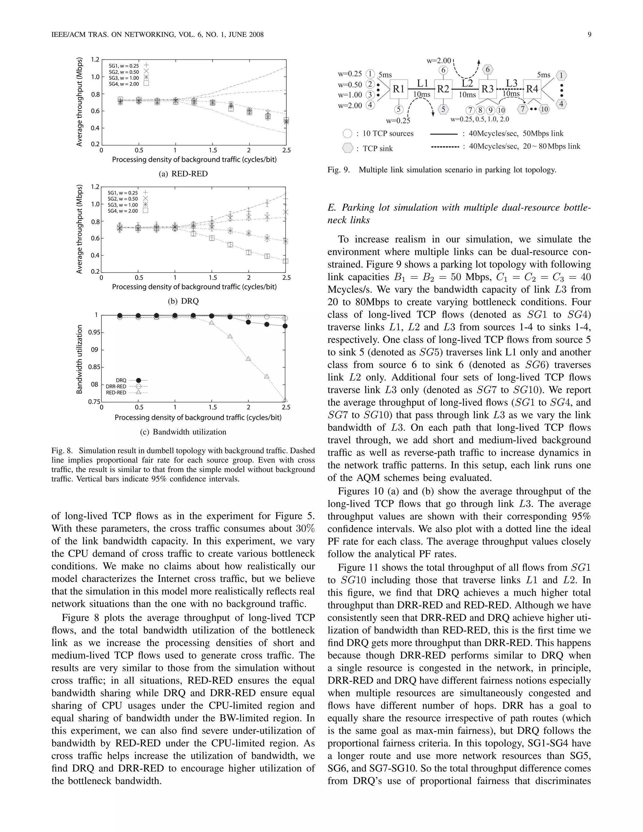
Figure 6 shows that the aggregate throughput achieved link is in the jointly-limited region which is the reason why
by each scheme. It shows that RED-RED has much lower the CPU share of high-processing flows go beyond 20%.
bandwidth utilization than the two other schemes. This is be-
cause, as discussed in Section II-B, when CPU is a bottleneck D. Dumbell with background Internet traffic
resource, the equilibrium operating points of TCP flows over No Internet links are without cross traffic. In order to
the RED CPU queue that achieve the equal bandwidth usage emulate more realistic Internet environments, we add cross
while keeping the total CPU usage below the CPU capacity traffic modelled from various observations on RTT distribu-
are much lower than those of the other schemes that need to tion [35], flow sizes [36] and flow arrival [37]. As modelling
ensure the equal sharing of CPU (not the bandwidth) under the Internet traffic in itself is a topic of research, we do not
the CPU-limited region. dwell on which model is more realistic. In this paper, we
present one model that contains the statistical characteristics
C. Impact of flows with high processing demands that are commonly assumed or confirmed by researchers.
In the introduction, we indicated that RED-RED can cause These characteristics include that the distribution of flow
extreme unfairness in use of resources. To show this by sizes has a long-range dependency [36], [38], the RTTs of
experiment, we construct a simulation run where we fix the flows is rather exponentially distributed [39] and the arrivals
CPU capacity to 40 Mcycles/s and add an increasing number of flows are exponentially distributed [37]. Following these
of flows with a high CPU demand (ws = 10) in the same setup characteristics, our cross traffic consists of a number of short
as the dumbell sink bottleneck environment in Section IV-B. and medium-lived TCP flows that follow a Poisson arrival
We call these flows high processing flows. From Figure 5, at process and send a random number of packets derived from
40 Mcycles/s, when no high processing flows are added, CPU a hybrid distribution of Lognormal (body) and Pareto (tail)
is not a bottleneck. But as the number of high processing distributions with cutoff 133KB (55% of packets are from
flows increases, the network moves into the CPU-limited flows larger than the cutoff size). We set the parameters of
region. Figure 7 shows the results of this simulation run. In flow sizes identical to those from Internet traffic characteristics
Figure 7 (a), as we increase the number of high processing in [36] (Lognormal:µ = 9.357, σ = 1.318, Pareto:α = 1.1), so
flows, the aggregate CPU share of high processing flows that a continuous distribution of flow sizes is included in the
deviates significantly from the equal CPU share; under a larger background traffic. Furthermore, we also generate reverse-path
number of high processing flows (e.g., 10 flows), these flows traffic consisting of 10 long-lived TCP flows and a number of
dominate the CPU usage over the other lower processing short and medium-lived flows to increase realism and also to
density flows, driving them to starvation. In contrast, DRQ and reduce the phase effect. The RTT of each cross traffic flow
DRR approximately implement the equal CPU sharing policy. is randomly selected from a range of 20 to 60 ms. We fix
Even though the number of high processing flows increases, the bottleneck bandwidth and CPU capacities to 40 Mbps
the bandwidth remains a bottleneck resource as before, so the and 40 Mcycles/s, respectively, and generate the same number](https://image.slidesharecdn.com/dual-resourcetcpaqm-120715130822-phpapp01/75/Dual-resource-TCPAQM-for-Processing-constrained-Networks-8-2048.jpg)
![IEEE/ACM TRAS. ON NETWORKING, VOL. 6, NO. 1, JUNE 2008 10
0.6
Average throughput (Mbps)
L3 bandwidth utilization
SG 1, w=0.25 1
SG 2, w=0.50
0.5 SG 3, w=1.0 0.95
SG 4, w=2.0 0.9
0.4 PF rate - SG1
PF rate - SG2 0.85
PF rate - SG3
0.3 PF rate - SG4 0.8
0.75
0.2
0.7
DRQ
0.1 0.65 DRR-RED
RED-RED
0.6
0 20 30 40 50 60 70 80
20 30 40 50 60 70 80
L3 link bandwidth (Mbps) L3 link bandwidth (Mbps)
(a) Fig. 12. L3 link bandwidth utilization comparison between DRQ, DRR-RED,
2.5 and RED-RED.
Average throughput (Mbps)
SG 7, w=0.25
SG 8, w=0.50
2 SG 9, w=1.0
SG10, w=2.0 SG4 SG5
PF rate - SG7 Access network
1.5 PF rate - SG8
PF rate - SG9 100Mbps
PF rate - SG10 SG3 [5~10]ms IE3 IE4
1 No
processing IE2 EE2
Core network
0.5 flows
100Mbps L1 L2
C1 C2 C3
0 SG2 5ms 40Mbps 60Mbps
20 30 40 50 60 70 80 Low 10ms 10ms EE1
IE1
L3 link bandwidth (Mbps) processing
flows EE3 EE4
(b)
SG1
Fig. 10. Throughput of TCP/DRQ in multiple link simulations: (a) SG1- High processing flows
SG4, (b) SG7-SG10. Even in cases where multiple links are dual-resource
constrained, DRQ achieves proportional fairness. Vertical bars indicate 95% Fig. 13. Simulation topology for edge deployment
confidence intervals.
105
DRQ F. Impact of incremental deployment
100 DRR-RED
Total throughput (Mbps)
RED-RED
95
In this section, we examine the performance impact of
90
85 incrementally deploying DRQ in the current Internet. The
80 natural places where DRQ can be initially deployed are likely
75 to be edges. This is because the current Internet trend is to keep
70
65
the “middle” slim by pushing complicated tasks to the edges of
60 the Internet. Thus, while core routers focus on moving packets
20 30 40 50 60 70 80
L3 link bandwidth (Mbps)
as fast as possible, routers, proxies and gateways located at
edges of the Internet perform various in-network processing
Fig. 11. Total throughput comparison between DRQ, DRR-RED, and RED- on packets.
RED. It shows the sum of throughput for all flows from SG1 to SG10. In We consider an ISP environment where core routers and
this setup, DRQ achieves the best throughput over the other schemes. This
is because the PF rate allocation of DRQ installs fairness among flows that most edge routers are free from processing constraint but a
traverse different numbers of hops. RED-RED still consistently shows lower small number of designated edge gateways handle TCP flows
throughput. with in-network processing requirement. Figure 13 models one
example of such environments. Our goal is to assess whether a
small incremental deployment of DRQ gives any performance
SG1-SG4 over the other flows because it uses more hops. advantage while keeping the rest of the network intact. In
The comparison of L3 link utilization shows that DRQ and the figure, SG’s denote TCP source groups, each with ten
DRR-RED use nearly the same amount, in Figure 12. This is TCP sources, and C1 to C3 denote core routers, IE1 to IE4
because L3 lies in the CPU-limited region so the bandwidth denote ingress edge routers and EE1 to EE4 denote egress edge
usage of the flows is governed by the fair usage of CPU. This routers, respectively. Flows from IE1 are routed through the
means that the bandwidth usage difference between SG1-SG4, shortest path to EE1 and etc. In this setup, all the routers except
and the other flows occur because of SG5 and SG6 flows that IE1 and EE1 are conventional packet routers with no CPU
traverse only one link creating a bandwidth bottleneck on their constraint and IE1 and EE1 are the media gateways/routers
corresponding link. However, it is incorrect to say that the that may run in the CPU-limited region.
fairness notion of DRQ always guarantees higher throughput In this simulation, we consider two different source groups,
than the fairness notion that DRR-RED follows as it is quite SG1 and SG2, that traverse the same end-to-end path from
possible that there are other unique situations where DRR- IE1 to EE1. SG1 consists of flows with a high processing
RED gets more throughput (which is indeed shown in the density (w1 = 2.5) while SG2 consists of flows with a low
next simulation). We leave as future study, studying the exact processing density (w2 = 0.5). Flows from SG3 to SG5 do
conditions where DRR-RED can have better throughput than not require any CPU processing. Note also that in this setup,
DRQ and vice versa. SG1, SG2 and SG3 share the same bottleneck links (L1 and](https://image.slidesharecdn.com/dual-resourcetcpaqm-120715130822-phpapp01/75/Dual-resource-TCPAQM-for-Processing-constrained-Networks-10-2048.jpg)
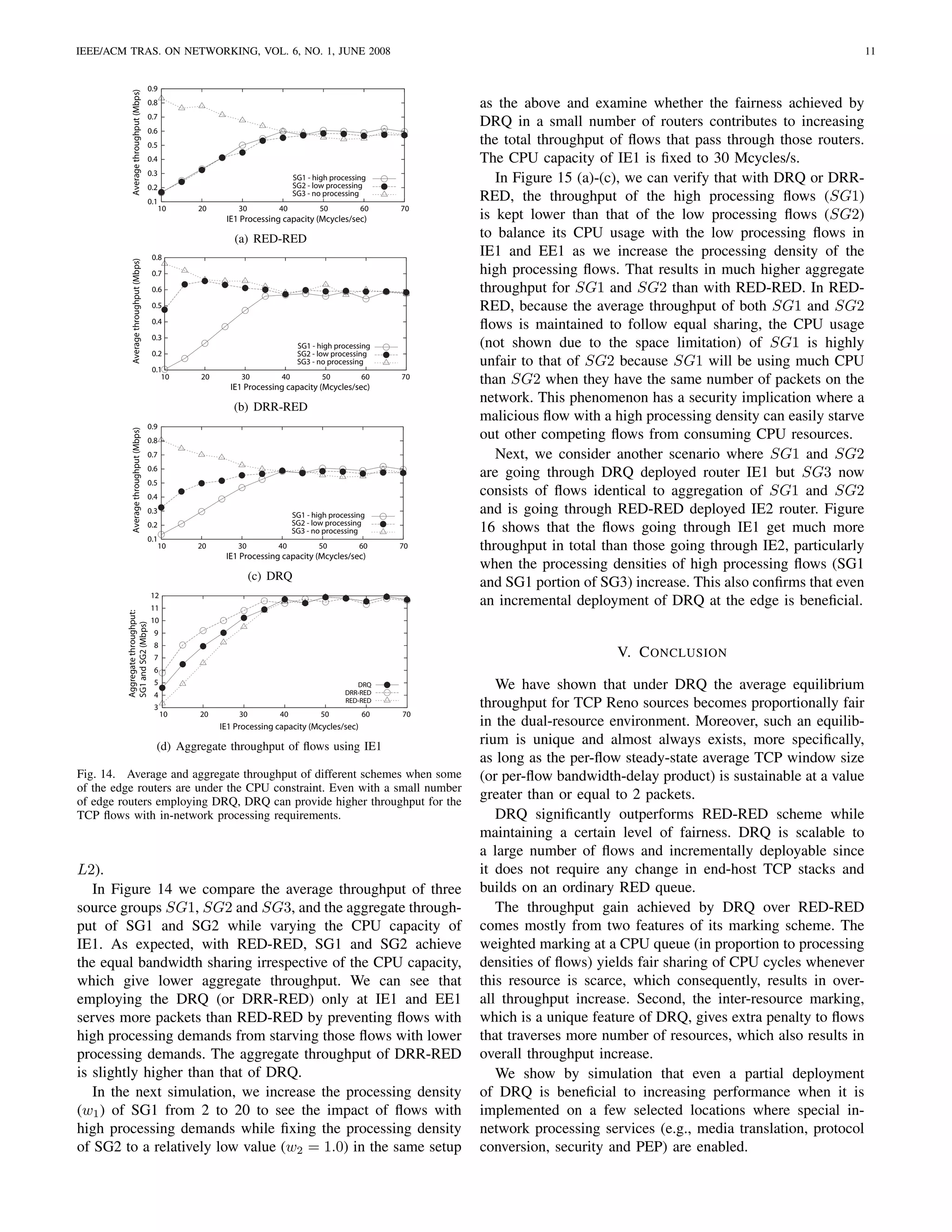
![IEEE/ACM TRAS. ON NETWORKING, VOL. 6, NO. 1, JUNE 2008 12
1
11
Average throughput (Mbps)
Aggregate throughput (Mbps)
10
0.8
9
0.6 8
7
SG1 - high processing
0.4 SG2 - low processing 6
SG3 - no processing 5
0.2 4
3 SG1 and SG2
0 SG 3
2 4 6 8 10 12 14 16 18 20 2
2 4 6 8 10 12 14 16 18 20
Processing density of SG1 (cycles/bit) Processing density of SG1 (cycles/bit)
(a) RED-RED
Fig. 16. Aggregate throughput comparison of flows going through DRQ
1
deployed router and flows going through RED-RED deployed router.
Average throughput (Mbps)
0.8
0.6
0.4
SG1 - high processing services at network edges,” in Proc. of IEEE Open Architectures and
SG2 - low processing
SG3 - no processing Network Programming (OPENARCH), San Francisco, CA, 2003.
0.2 [7] S. Chong, M. Shin, J. Mo, and H.-W. Lee, “Flow control with processing
constraint,” IEEE Commun. Lett., vol. 9, no. 10, pp. 957–959, Oct. 2005.
0
2 4 6 8 10 12 14 16 18 20 [8] A. Demers, S. Keshav, and S. Shenker, “Analysis and simulation of a
Processing density of SG1 (cycles/bit) fair queueing algorithm,” ACM SIGCOMM Computer Communications
Review, vol. 19, no. 4, pp. 1–12, 1989.
(b) DRR-RED
[9] M. Shreedhar and G. Varghese, “Efficient fair queueing using deficit
1 round robin,” in Proc. of ACM SIGCOMM, Sept. 1995, pp. 231–242.
Average throughput (Mbps)
0.8
[10] S. Floyd and V. Jacobson, “Random Early Detection gateways for
congestion avoidance,” IEEE/ACM Trans. Networking, vol. 1, pp. 397–
0.6 413, Aug. 1993.
[11] S. Athuraliya, S. H. Low, V. H. Li, and Q. Yin, “REM: Active queue
0.4 SG1 - high processing
SG2 - low processing management,” IEEE Network, vol. 15, pp. 48–53, May 2001.
0.2 SG3 - no processing [12] C. V. Hollot, V. Misra, D. Towsley, and W. B. Gong, “On designing
improved controllers for AQM routers supporting TCP flows,” in Proc.
0
2 4 6 8 10 12 14 16 18 20 of IEEE INFOCOM, Anchorage, Alaska, Apr. 2001, pp. 1726–1734.
Processing density of SG1 (cycles/bit) [13] I. Stoica, S. Shenker, and H. Zhang, “Core-stateless fair queueing:
Achieving approximately fair bandwidth allocations in high speed net-
(c) DRQ works,” in Proc. of ACM SIGCOMM, Sept. 1998, pp. 118–130.
12 [14] Z. Cao, Z. Wang, and E. W. Zegura, “Rainbow fair queueing: Fair
11
bandwidth sharing without per-flow state,” in Proc. of IEEE INFOCOM,
Aggregate throughput:
10
SG1 and SG2 (Mbps)
9 Tel Aviv, Israel, Mar. 2000, pp. 922–931.
8 [15] P. Pappu and T. Wolf, “Scheduling processing resources in program-
7
6
mable routers,” in Proc. of IEEE INFOCOM, New York, NY, June 2002,
5 pp. 104–112.
4 DRQ
DRR-RED
[16] F. Sabrina, C. D. Nguyen, S. K. Jha, D. Platt, and F. Safaei, “Processing
3
RED-RED resource scheduling in programmable networks,” Computer Communi-
2
2 4 6 8 10 12 14 16 18 20 cations, vol. 28, no. 6, pp. 676–687, Apr. 2005.
Processing density of SG1 (cycles/bit) [17] T. Wolf and M. A. Franklin, “CommBench - a telecommunications
(d) Aggregate throughput of flows using IE1 benchmark for network processors,” in Proc. of IEEE International
Symposium on Performance Analysis of Systems and Software (ISPASS),
Fig. 15. Average and aggregate throughput when processing density values Austin, TX, Apr. 2000, pp. 154–162.
of neighboring flows (SG1) are increased. This shows that DRQ and DRR- [18] G. Memik, M. Smith, and W. Hu, “NetBench: A benchmarking suite
RED, even in a partial deployment, achieve fairness in the CPU usage when for network processors,” in Proc. of IEEE International Conference on
some portion of flows has increasingly higher processing demands. Computer-Aided Design, San Jose, CA, Nov. 2001, pp. 39–42.
[19] M. Tsai, C. Kulkarni, C. Sauer, N. Shah, and K. Keutzer, “A bench-
marking methodology for network processors,” in Proc. of 1st Network
Processor Workshop, 8th Int. Symp. on High Performance Computer
R EFERENCES Architectures (HPCA), Cambridge, MA, Feb. 2002.
[20] F. P. Kelly, A. K. Maulloo, and D. K. H. Tan, “Rate control in commu-
nication networks: shadow prices, proportional fairness and stability,” J.
[1] R. Ramaswamy, N. Weng, and T. Wolf, “Analysis of network processing of the Operational Research Society, vol. 49, pp. 237–252, Apr. 1998.
workloads,” in Proc. of IEEE International Symposium on Performance [21] S. H. Low and D. E. Lapsley, “Optimization flow control I: Basic
Analysis of Systems and Software (ISPASS), Austin, TX, Mar. 2005, pp. algorithm and convergence,” IEEE/ACM Trans. Networking, vol. 7, pp.
226–235. 861–875, Dec. 1999.
[2] P. Crowley, M. E. Fiuczynski, J.-L. Baer, and B. N. Bershad, “Workloads [22] D. P. Bertsekas, Nonlinear Programming, 2nd ed. Belmont, MA:
for programmable network interfaces,” in Workload Characterization for Athena Scientific, 1999.
Computer System Design. Kluwer Academic Publishers, 2000, ch. 7. [23] S. H. Low, “A duality model of TCP and queue management algorithms,”
[3] Y. Gottlieb and L. Peterson, “A comparative study of extensible routers,” IEEE/ACM Trans. Networking, vol. 11, pp. 525–536, Aug. 2003.
in Proc. of IEEE Open Architectures and Network Programming (OPE- [24] F. P. Kelly, “Mathematical modelling of the internet,” in Mathematics
NARCH), June 2002, pp. 51–62. Unlimited – 2001 and Beyond, B. Engquist and W. Schmid, Eds. Berlin:
[4] A. T. Campbell, H. G. D. Meer, M. E. Kounavis, K. Miki, J. B. Vicente, Springer Verlag, 2001, pp. 685–702.
and D. Villela, “A survey of programmable networks,” ACM SIGCOMM [25] V. Misra, W. B. Gong, and D. Towsley, “Fluid-based analysis of a
Computer Communications Review, vol. 29, no. 2, pp. 7–23, April 1999. network of AQM routers supporting TCP flows with an application to
[5] A. Barbir, R. Penno, R. Chen, M. Hofmann, and H. Orman, “An RED,” in Proc. of ACM SIGCOMM, Sept. 2000, pp. 151–160.
architecture for open pluggable edge services (OPES),” IETF RFC 3835, [26] Y. Liu, F. Presti, V. Misra, and D. Towsley, “Fluid models and solutions
2004. for large-scale IP networks,” in Proc. of ACM SIGMETRICS, San Diego,
[6] B. Falchuk, J. Chiang, A. Hafid, Y.-H. Cheng, N. Natarjan, F. J. Lin, CA, June 2003, pp. 151–160.
and H. Cheng, “An open service platform for deploying and managing [27] C. V. Hollot, V. Misra, D. Towsley, and W.-B. Gong, “A control theoretic](https://image.slidesharecdn.com/dual-resourcetcpaqm-120715130822-phpapp01/75/Dual-resource-TCPAQM-for-Processing-constrained-Networks-12-2048.jpg)
![IEEE/ACM TRAS. ON NETWORKING, VOL. 6, NO. 1, JUNE 2008 13
analysis of RED,” in Proc. of IEEE INFOCOM, Anchorage, Alaska, Apr. Lagrangian optimality condition of Problem P, we need to
2001, pp. 1510–1519. show that
[28] S. H. Low, F. Paganini, J. Wang, and J. C. Doyle, “Linear stability
of TCP/RED and a scalable control,” Computer Networks, vol. 43, pp. αs
633–647, Dec. 2003. x∗ =
s k σ∗ + ∗, ∀s∈S (33)
[29] “Internet end-to-end performance monitoring group (IEPM),” 2006. k∈K(s) ws k l∈L(s) ρl
[Online]. Available: http://www-iepm.slac.stanford.edu/ ∗
[30] K. Ramakrishnan and S. Floyd, “A proposal to add explicit congestion hold. Consider flow s. If we suppose that σk = 0, ∀k ∈ K(s),
notification (ECN) to IP,” IETF RFC 2481, 1999. ∗
and ρl = 0, ∀l ∈ L(s), for this flow s, then p∗ = 0 from
s
[31] K. Ramakrishnan, S. Floyd, and D. Black, “The addition of explicit Eq. (15), which contradicts Eq. (9) since it cannot have an
congestion notification (ECN) to IP,” IETF RFC 3168, 2001.
[32] H. Han, C. V. Hollot, Y. Chait, and V. Misra, “TCP networks stabilized equilibrium point satisfying p∗ = 0. Thus, at least one of σk ,
s
∗
∗
by buffer-based AQMs,” in Proc. of IEEE INFOCOM, Hongkong, Mar. k ∈ K(s), and ρl , l ∈ L(s), must be positive, which implies
2004, pp. 964–974. that 0 < p∗ < 1 from Eq. (15) and consequently x∗ > 0 ∗ from
[33] “ns-2 network simulator,” 2000. [Online]. Available: s s
M (1−p )
http://www.isi.edu/nsnam/ns/ Eq. (9). Therefore, from Eq. (9), we know that s τ 2 s =
s
[34] S. Floyd, “Recommendations on using the gentle variant of RED,” Mar. ∗2 ∗
2 xs ps
2000. [Online]. Available: http://www.aciri.org/floyd/red/gentle.html 3 Ms (Ns is cancelled out). Solving x∗ from this equation by
s
[35] J. Aikat, J. Kaur, F. D. Smith, and K. Jeffay, “Variability in TCP round- substituting Eq. (15) at equilibrium for p∗ , we get Eq. (33) with
√ s
trip times,” in Proc. of 3rd ACM SIGCOMM Conference on Internet 3/2M s
Measurement Conference, Oct. 2003, pp. 279–284. αs = τs , which concludes the Lagrangian optimality of
[36] P. Barford and M. Crovella, “Generating representative web workloads (x , σ , ρ ). Lastly, we need to show that σk ( s∈S(k) ws x∗ −
∗ ∗ ∗ ∗ k
s
for network and server performance evaluation,” in Proc. of ACM
SIGMETRICS, July 1998, pp. 151–160. Ck ) = 0 and ρ∗ ( s∈S(l) x∗ −Bl ) = 0 for all k ∈ K and l ∈ L
l s
[37] V. Paxson and S. Floyd, “Wide-area traffic: The failure of poisson to check complementary slackness of (x∗ , σ ∗ , ρ∗ ). Consider
modeling,” IEEE/ACM Trans. Networking, vol. 3, pp. 226–244, June arbitrary k ∈ K. If we suppose that s∈S(k) ws x∗ − Ck < 0,
k
s
1995. ∗ ∗
[38] K. Park, in Self–Similar Network Traffic and Performance Evaluation, ˆ∗
then zk = vk = 0 from Eq. (8). Thus, vk = 0 from Eq. (14)
∗
W. Willinger, Ed. New York: John Wiley & Sons, 2000. and consequently σk = 0 from Eq. (13), which concludes
[39] H. Jiang and C. Dovrolis, “Passive estimation of TCP round-trip times,” σk ( s∈S(k) ws x∗ − Ck ) = 0. Similarly, ρ∗ ( s∈S(l) x∗ −
∗ k
s l s
ACM SIGCOMM Computer Communications Review, vol. 32, pp. 75–
88, July 2002. Bl ) = 0 for arbitrary l ∈ L. Therefore, we conclude that
(x∗ , σ ∗ , ρ∗ ) is the primal-dual optimal solution of Problem P.
A PPENDIX Moreover, x∗ is unique since the optimal solution of Problem
∗
P is unique. From Eq. (10), it is obvious that yl > bl if
Proof of Proposition 1: First, we show that the √ primal- ρ∗ > 0 and 0 ≤ yl ≤ bl otherwise. The same argument can
∗
3/2Ms l
∗ ∗ ∗
optimal solution (r , θ , π ) of Problem P with αs = τs be applied to CPU queues from Eq. (13).
forms an equilibrium point (x , σ , ρ , p , y , z , v ∗ ,
∗ ∗ ∗ ∗ ∗ ∗
Proof of Proposition 2: First, we derive a linearized model
y ∗ , v ∗ ) in the average Reno/DRQ network where x∗ =
ˆ ˆ of Reno/DRQ network at the equilibrium point. In the DRQ
r∗ , σ ∗ = θ∗ , ρ∗ = π ∗ if θ∗ and π ∗ satisfy C1 and C2. network described by Eq. (15), the congestion window for
∗ k ∗
Since s∈S(l) rs ≤ Bl , ∀l ∈ L, and s∈S(k) ws rs ≤ Ck , the sth TCP source, s , can be modelled by the nonlinear
∗
∀k ∈ K, Eqs. (7) and (8) imply that there exist yl ≥ 0, differential equation
∗ ∗
∀l ∈ L, and zk , vk ≥ 0, ∀k ∈ K. Thus, from Eqs. (11) and 2
ˆ∗ ∗
ˆ∗
(14), there exist yl = yl ≥ 0, ∀l ∈ L, and vk = vk ≥ 0,∗ 1 − ps (t) 2 s (t)
˙ s (t) = − ps (t) (34)
∀k ∈ K, whose specific values can be obtained from Eqs. N s τs 3Ns τs
(10) and (13) for ρ∗ = πl and σk = θk since 0 ≤ πl < 1
l
∗ ∗ ∗ ∗
where,
∗ ∗
and 0 ≤ θk < 1. Finally, for xs > 0, Eqs. (9) and (15)
√ 2
3/2M |R| T
yield x∗ = ( k∈K(s) ws σk + l∈L(s) ρ∗ )−1 , which i=1 [Γ(0) ]si ϕi (t − τis )
s k ∗
s τs l
∗ ∗ ∗
also holds for (r , θ , π ) by the Lagrangian optimality of ps (t) = 2 (35)
√ |R| T
3/2M 1+ i=1 [Γ(0) ]si ϕi (t − τis )
(r∗ , θ∗ , π ∗ ) in Eq. (6) with αs = τs
s
.
Next we prove the converse that if the average Reno/DRQ and ϕi (t) is the ith element of unified pre-marking probability
network has an equilibrium point (x∗ , σ ∗ , ρ∗ , p∗ , y ∗ , z ∗ , v ∗ , set as
y ∗ , v ∗ ), then (x∗ , σ ∗ , ρ∗ ) is the primal-dual optimal solution
ˆ ˆ √ σi if i indicates CPU
3/2M ϕi =
of the corresponding Problem P with αs = s
and, ρi if i indicates link
τs
moreover, no other equilibrium points can exist in the network.
Using Eqs. (7)-(8), we model the ith congested resource
By the duality theory [22], the necessary and sufficient con-
queue by
dition for (x∗ , σ ∗ , ρ∗ ) to be the primal-dual optimal solution
of Problem P is that x∗ is primal feasible, (σ ∗ , ρ∗ ) is dual |S|
Ms s (t − τis )
feasible, and (x∗ , σ ∗ , ρ∗ ) satisfies Lagrangian optimality and qi (t) = −˜i Iq>0 +
˙ c [Γis (0)] (36)
complementary slackness. First, Eqs. (7) and (8) imply that s=1
τs
∗ k ∗
s∈S(l) xs ≤ Bl for all l ∈ L and s∈S(k) ws xs ≤ Ck where qi (t) is the ith element of the resource queue length set
for all k ∈ K, and Eq. (9) implies that x ≥ 0. Thus, x∗
∗
in bits (or cycles) as
is primal feasible. Second, the dual feasibility of (σ ∗ , ρ∗ ) is
obvious since σ ∗ and ρ∗ cannot be negative by the definition zi if i indicates CPU
qi =
of REDs in Eqs. (10) and (13). Third, since Eq. (6) is the yi if i indicates link,](https://image.slidesharecdn.com/dual-resourcetcpaqm-120715130822-phpapp01/75/Dual-resource-TCPAQM-for-Processing-constrained-Networks-13-2048.jpg)
![IEEE/ACM TRAS. ON NETWORKING, VOL. 6, NO. 1, JUNE 2008 14
ci is the ith element of resource capacity set as
˜ Minsu Shin (S’99) received his B.S., M.S., and
Ph.D. degrees in the School of Electrical Engineer-
Ci if i indicates CPU ing and Computer Science, Korea Advanced Institute
ci =
˜
Bi if i indicates link, of Science and Technology (KAIST), Daejeon, Ko-
rea, in 1998, 2000, and 2006, respectively. From July
Ms denotes the packet size in bits, and Iq>0 is the indicator 2006, he is a Visiting Postdoctoral Research Fellow
function. at the Dept. of Computer Science, North Carolina
Linearizing Eqs. (34)-(36) about equilibrium ( ∗ , q ∗ , ϕ∗ ) State University, Raleigh. His research interests are
in congestion control, programmable networks, and
and taking Laplace transforms gives wireless networks.
˜
(z) = −F (z)Γ(−z)T ϕ(z) (37)
q(z) = (zI + Ω)−1 Γ(z)M T −1 (z) (38)
˜ ˜
where F (z) = diag{fs (z)},
˜ e−zτs 2
fs (z) = 4 s∗ ,
z+ 3
∗2
Ns τs u∗ (1 + u∗ )2
s s
3Ns τs 2 s +3
˜
u∗ = Γ(0)T ϕ∗ , Ω = Γ(0)M W ∗ T −2 Γ(0)T C −1 , T =
diag{τs }, M = diag{Ms }, W ∗ = diag{ s } and C =
∗ ˜
diag{˜i }.
c
Next, let κi (z) denote the linearized RED dynamics which
Song Chong (M’93) received the B.S. and M.S.
can be modelled as the low-pass filter [25], degrees in Control and Instrumentation Engineering
ϕi (z) ψi from Seoul National University, Seoul, Korea, in
κi (z) = = (39) 1988 and 1990, respectively, and the Ph.D. degree
qi (z) z/ηi + 1 in Electrical and Computer Engineering from the
University of Texas at Austin in 1995. Since March
where ψi = b mi , and η = loge (1−λ) , where h is sampling
h 2000, he has been with the School of Electrical En-
i −bi
interval of RED. Using linearized Eqs. (37)-(39), we can find gineering and Computer Science, Korea Advanced
Institute of Science and Technology (KAIST), Dae-
the return ratio function of the DRQ network. jeon, Korea where he is an Associate Professor,
˜ ˜
L(z) = F (z)Γ(−z)T D(z)C −1 (zI + Ω)−1 Γ(z)M T −1 (40) leading the Network Systems Laboratory. Prior to
joining KAIST, he was with the Performance Analysis Department, AT&T
where D(z) = diag{κi (z)˜i }. To invoke the Generalized
c Bell Laboratories, Holmdel, New Jersey, as a Member of Technical Staff.
His research interests include high speed networks, wireless networks and
Nyquist Stability Criterion [32], we should show that the performance evaluation. He has published more than 60 papers in international
eigenvalues of L(jw) do not intersect (−∞, −1] for all w ≥ 0. journals and conferences and holds three U.S. patents in these areas. He is
From Theorem 1 and Proposition 1 in [32], these eigenval- an Editor of the Journal of Communications and Networks and has served
as a Technical Program Committee member of a number of international
ues lie in conferences
max{|fs (jw)|}max{|di (jw)|}
, (41)
min{|gi (jw)|}
˜
where fs (jw) = µs fs (jw), µs is the number of congested
s
resources traversed by the sth source, di (jw) = κi (jw) · ci ,
˜
˜ 1 ˜ 1
gi (jw) = jw + λi , and λi is an eigenvalue of C − 2 ΩC − 2 . To
be stable, Eq.(41) should be less than 1.
Because min{|gi (jw)|} is an increasing function,
max{|fs (jw)|} and max{|di (jw)|} are decreasing, stability
condition can be replaced by,
max{|fs (0)|}max{|di (0)|}
< 1. (42) Injong Rhee (SM’89) received his Ph.D. from the
min{|gi (0)|}
University of North Carolina at Chapel Hill. He is
We can find the following relations an associate professor of Computer Science at North
Carolina State University. His areas of research inter-
φ2 [Γ(0)]
min ests include computer networks, congestion control,
|gi (0)| ≥ 2
(43)
Λmax τmax wmax wireless ad hoc networks and sensor networks. He
works mainly on network protocol designs optimiz-
|R|Λmax τmax ing the transport performance of networks.
|fs (0)| ≤ (44)
3/2
where Λmax = max{ min{wk } min{Ms } , min{Ms} }, τmax =
max{Ck } max{Bl
}
s
k
max{τs }, wmax = max{ws , 1} and φmin [Γ(0)] denotes the
smallest singular values of the matrix Γ(z) evaluated at z = 0.
From the Eqs. (42)-(44),
3/2φ2 [Γ(0)]
min
max{|di (0)|} ≤ . (45)
|R|Λ2 τmax wmax
max
3](https://image.slidesharecdn.com/dual-resourcetcpaqm-120715130822-phpapp01/75/Dual-resource-TCPAQM-for-Processing-constrained-Networks-14-2048.jpg)

This document summarizes a research paper that examines congestion control issues for TCP flows that require in-network processing by network elements like routers. It proposes a new active queue management (AQM) scheme called Dual-Resource Queue (DRQ) that can approximate proportional fairness for bandwidth and CPU resources without changing TCP stacks. The study finds that current TCP/AQM schemes can lose throughput and cause unfairness in networks where CPU cycles are scarce. DRQ maintains separate queues for each resource and works with classes of flows based on their known processing requirements, making it scalable without per-flow state. Simulation results show DRQ achieves fair and efficient resource allocation with low implementation costs.