Estimating Parameters of Multiple Heterogeneous Target Objects Using Composite Sensor Nodes

This article has been accepted for publication in a future issue of this journal, but has not been fully edited. Content may change prior to final publication.
IEEE TRANSACTIONS ON MOBILE COMPUTING

1

Estimating Parameters of Multiple
Heterogeneous Target Objects Using Composite
Sensor Nodes
Hiroshi Saito, Fellow, IEEE, Shinsuke Shimogawa, Sadaharu Tanaka, and Shigeo Shioda, Member, IEEE

Abstract—We propose a method for estimating parameters of multiple target objects by using networked binary sensors whose
locations are unknown. These target objects may have different parameters, such as size and perimeter length. Each sensors, which is
incapable of monitoring the target object’s parameters, sends only binary data describing whether or not it detects target objects coming
into, moving around, or leaving the sensing area at every moment. We previously developed a parameter estimation method for a single
target object. However, a straight-forward extension of this method is not applicable for estimating multiple heterogeneous target objects.
This is because a networked binary sensor at an unknown location cannot provide information that distinguishes individual target
objects, but it can provide information on the total perimeter length and size of multiple target objects. Therefore, we propose composite
sensor nodes with multiple sensors in a predetermined layout for obtaining additional information for estimating the parameter of each
target object. As an example of a composite sensor node, we consider a two-sensor composite sensor node, which consists of two
sensors, one at each of the two end points of a line segment of known length. For the two-sensor composite sensor node, measures
are derived such as the two sensors detecting target objects. These derived measures are the basis for identifying the shape of each
target object among a given set of categories (for example, disks and rectangles) and estimating parameters such as the radius and
lengths of two sides of each target object. Numerical examples demonstrate that networked composite sensor nodes consisting of two
binary sensors enable us to estimate the parameters of target objects.

Index Terms—Sensor network, estimation, target object, composite sensor node, ubiquitous network, integral geometry, geometric
probability.

✦

1 I NTRODUCTION extract signiﬁcant information. This sensing paradigm is
appropriate for the described situation.
Small and low-cost sensors can be used to build wireless
Unfortunately, we have not determined a theory that
sensor networks [1], [2], [3]. They have communication
enables us to implement this paradigm. As a typical
capabilities and built-in batteries to communicate via a
and challenging application, we investigated a problem
wireless link for transmitting sensed data of detected
of estimating parameters related to the shape and size
events of interest. A newly proposed development, such
of target objects moving in a monitored area by using
as a wide area ubiquitous network [4], supports sensors
many simple randomly distributed sensors. We address
with low performance and functionalities and a long-
this problem and present a theory for estimating the
range, low-speed wireless link with very low power con-
parameters of multiple target objects by using networked
sumption. These sensors can be implemented as single
binary sensors whose locations are unknown. An in-
chips, lowering their cost. As a result, we can deploy
dividual sensor is simple. It monitors its environment
such sensors like the scattering of dust [5]. Because there
and reports whether or not it detects a target object. It
are many sensors, we cannot carefully design the loca-
does not have a positioning function, such as a GPS, or
tion of each one. GPS cannot be used because the sensors
functions for monitoring the target object size and shape,
should have limited capability and power consumption.
such as a camera, and it can be placed without careful
This situation leads us to a new sensing paradigm.
design. However, by collecting reports from individual
That is, instead of having a few sensors with advanced
sensors, we can statistically estimate the parameters of
functions and high performance, many sensors with
target objects.
simple functions and low performance are distributed
In addition to theoretical contributions, this work is
randomly. They are networked and send reports, each of
useful to some application scenarios that require low
which includes only an insigniﬁcant amount of informa-
cost, a wide coverage, and low power consumption
tion, over a wireless link. However, as a whole, we can
and accept rough estimation of the size and shape of
target objects. For example, we may need to identify the
¯ H. Saito and S. Shimogawa are with NTT Service Integration Laboratories,
3-9-11, Midori-cho, Musashino-shi, Tokyo, 180-8585, Japan.
number and kinds of animals and vehicles in a large
E-mail: saito.hiroshi@lab.ntt.co.jp area to observe the wildlife, prevent poaching, or limit
¯ S. Tanaka and S. Shioda are with Chiba University. the number of tourist vehicles. We can easily obtain bi-
nary sensors of sound volume, acceleration, infrared, or

Digital Object Indentifier 10.1109/TMC.2011.65 1536-1233/11/$26.00 © 2011 IEEE


2

magnetic sensors for such scenarios. These sensors with for such a purpose. In particular, [8] and [14] directly
normal detection ranges are not expensive. Therefore, we apply the results of integral geometry discussed in
can provide a large number of these sensors to cover a Chapter 5 and Section 6.7 in [15] to the analysis of
large area at a reasonable cost. By distributing these bi- detecting an object moving in a straight line and to the
nary sensors without expensive power-consuming GPSs evaluation of the probability of -coverage. In addition,
or time-consuming carefully-designed placement in a [16] applies integral geometry to the analysis of straight
large area, our proposed method can work. line routing, which is an approximation of the shortest
This research is an extension of our prior study [6], path routing, and [17] uses it to operate sensors in an
which was based on the coverage process theory [7] energy-conserving way.
and its application to sensor networks [8], [9], [10]. This The rest of this paper is organized as follows.
study emphasized the robustness of the derived formula Section 2 describes a basic model and previous results
for a number of sensors detecting a target object. In for the model. In Section 3, we introduce composite
[6], sensors that measure the size of a detected part sensor nodes and describe an extended model (static
of a target object are used for estimating the overall submodel). We discuss the analysis for deriving mea-
size. However, in [11], we developed a shape and size sures in Section 4. In Section 5, we discuss the dynamic
estimation method using binary sensors for sending submodel of the extended submodel. We then propose
reports on whether or not they detect the target object. an estimation method that uses composite sensor nodes
That study assumed that both the target object and the for target objects with different parameters in Section 6.
sensing area are convex or that the sensing area is disk- We show numerical examples in Section 7, and conclude
shaped. This developed method [11] was evaluated in this paper in Section 8.
an experiment where the target object was a box and
the sensor was an infrared distance measurement sensor
[12]. We also extended the estimation method in [11] to 2 P REVIOUS WORK
apply to non-convex target objects [13].
2.1 Basic model
These methods we developed in [11], [13] did not
take into account when multiple target objects are in the To describe the results of the previous work, which is
monitored area. This work addresses such a case, i.e., the basis of the current work, we discuss the basic model
multiple target objects that may have different shapes that the previous work used.
and sizes coming into, moving around, and leaving the A sensor network operator deploys sensors in a con-
area monitored by sensors. Each sensor, whose location vex area ¨ in 2-dimensional space Ê¾ , but the operator
is unknown, sends a report on whether or not at least does not know the sensor locations. Each sensor has
one target object is detected within its sensing area. The a sensing area, monitors the environment, and detects
sensor network operator collects these reports to identify events within that area. (This model is called the Boolean
the shape and to estimate parameters, such as sizes sensing model [9], [18], [19], [20] because it is clear
and perimeter lengths, of the target objects. However, whether a point is within a sensing area or not.) A sensor
identifying the shape and estimating the parameters of sends a detection report if a target object is in its sensing
multiple heterogeneous (i.e., having different parame- area, and it sends a no-detection report if there is no
ters) target objects is difﬁcult, and a straight-forward target object in that area. (It is possible to assume that a
extension of the estimation method we previously de- sensor does not send a report if there is no target object
veloped [11] is not applicable. Thus, we introduce the in that area and that the sensor network operator judges
concept of composite sensor nodes where multiple sim- no-detection if there is no report within a timeout. This
ple binary sensors are arranged in a predetermined scenario can reduce the power consumption of sensors,
layout, such as a line. Sensors in a composite sensor but the sensor network operator cannot distinguish no-
node provide local and relative information even if the detection from the loss of reports. For simplicity, this
location of that node is unknown. This is because the paper assumes that no-report is sent if there is no target
relative locations of these sensors are predetermined. In object in that area.)
this sense, the composite sensor node is an intermediate Assume that the -th sensor is located at ´Ü Ý µ and
concept between a simple and an advanced sensor node the sensing area is rotated by from the referenced
equipped with GPS. With these sensors, we can estimate position. Let ´Ü Ý µ Ê¾ be the sensing area
the parameters of multiple heterogeneous target objects. where ½ ¾ . The -th sensor has communication
The estimation method using composite sensor nodes capability and can send a report Á . Here, Á is 1 if
is derived from integral geometry and geometric prob- it detects the target object and 0 if otherwise. That is,
ability, which are useful tools for analyzing a geometric Á ½´ ´Ü Ý µ Ì µ, where ½´ µ is an indicator
or spatial structure. Ubiquitous access networks, such function that becomes 1 if a statement is true and 0 if
as wireless sensor networks, require analysis of the otherwise. At Ø Ø , the -th sensor sends a report, Á ´Ø µ,
geometric or spatial structure of an object, and there is describing whether or not it detects the target object. The
literature (including one of our papers [11]) describing sensor network operator receives the report from each
the use of integral geometry and geometric probability sensor through the network.


3

Sensors are classified into multiple types according to 3 C OMPOSITE SENSOR NODE
their sensing areas. That is, different types of sensors Estimating the unknown parameters of multiple target
have different sensing area sizes or shapes. (A different objects is difficult. Even when the number of target
sensing area can often be implemented by changing the objects is known, a straight-forward extension of the
sensitivity parameter of a sensor.) Type- sensors, of estimation method for a single target object to one for
which sensing area is denoted by , are deployed with multiple target objects is not applicable if the parameters
mean density . Assume that the first to Ò½ -th sensors of each target object are different. To estimate the pa-
are type-1 sensors, the ´Ò½ · ½µ-th to Ò¾ -th sensors are rameters of each target object, we introduce a composite
type-2 sensors, ... In general, Ò ½ · ½ ¡ ¡ ¡ Ò -th sensors
are type- sensors. Á
ØÑ
Ø Ø½
Ò È È
Ò ½ ·½ Á ´Øµ Ñ de-
sensor node, which consists of multiple sensors arranged
in a predetermined layout, such as a line. Instead of
notes the time average of the number of type- sensors deploying individual sensors, the sensor network op-
detecting the target object at each measurement epoch. erator deploys composite sensor nodes. Although the
We assume that the sensor network operator knows the locations of the composite sensor nodes are unknown,
sensor type of each sensor sending a report. local and relative information among multiple sensors
Consider a target object Ì in 2-dimensional space Ê¾ . in a predetermined layout of a composite sensor node
Its size is Ì , and its perimeter length is Ì . (In the becomes available because the relative locations of these
remainder of this paper, Ü denotes the size of Ü and sensors are known.
Ü denotes the perimeter length of Ü.)
Define a detectable area such that sensors will 3.1 Straight-forward extension to multiple target ob-
detect the target object if and only if they are located jects
in a detectable area with a certain rotation angle.
That is, ½´ ´Ü Ý µ Ì µ ½ if and only if
Before introducing composite sensor nodes, we explain
´Ü Ý µ ¾
an extension of Eq. (1) to an equation applicable to
. Equivalently, ´Ü Ý µ ´Ü Ý µ
Ì ÊÊÊ
. The detectable area size is defined as
multiple target objects.
Proposition 1: Assume that there are Ò Ì convex and
ÜÝ ¾
Ü Ý ¾ . We should note that
and Ì . When
bounded target objects and that the sensing area is
depends on both is disk-shaped,
also bounded and convex. Let be the detectable areas
of the -th target object and £
does not depend on . When does not depend on ,
´Ü Ý µ ´Ü Ý µ Ì
. If
we define for simplicity.
for any ,
Ì
Ò Ò Ì
2.2 Previous results for basic model
£ ½
´ Ì µ¡ · Ì · ÒÌ (5)
¾
½ ½
In this section, we summarize our previous results,
which are used in the current work. For the convex target
This is because
È
where Ì denotes the -th target object ´½
and because
ÒÌ µ. £
object, we have obtained the following equation, and a
shape and size estimation method was developed based satisfies Eq. (1).
Therefore, we can estimate
ÒÌ
½ Ì and
È ÒÌ
½ Ì
È
on this equation [11]: Assume that both the target object
Ì and the sensing area are bounded and convex. Then, instead of Ì and Ì in Eqs. (3) and (4), respectively.
Consequently, if we can assume that all the target objects
½
¾
Ì ¡ · Ì · (1)
have the same shape and size, we can estimate the size
and shape (size and perimeter length) of each target
object. However, if not, we cannot estimate the size and
Based on the fact that Á , we developed shape (size and perimeter length) of each target object
the following estimation method. (1) At Ø , receive the re-
È È
no matter how many types of sensors we introduce.
port Á ´Ø µ from each sensor whose location is unknown.
Ñ Ò
(2) Calculate Á ½ Ò ½ ·½ Á ´Ø µ Ñ for each
sensor type ( ½ ¾). (3) For two unknown parameters
3.2 Extended model (static submodel)
Ì and Ì , use Eq. (1) with the estimator Á of For analyzing an estimation method for multiple hetero-
and solve the following equations for ½ ¾. geneous target objects, we introduce a new model.
A sensor network operator deploys composite sensor
´
½
¾
Ì ¡ · Ì · µ Á (2) nodes in a convex area ¨ in 2-dimensional space Ê¾ , but
the operator does not know their locations. A composite
where Ì Ì are estimators of Ì Ì . That is,
sensor node consists of multiple sensors arranged in a
predetermined layout. We now consider a two-sensor

Ì ¾ ´Á½ ½ Á¾ ¾ ½ · ¾ µ
composite sensor node, i.e., a composite sensor node
½ ¾
(3) with two sensors. These two sensors are the same as
those described in the basic model. That is, they are
Ì ¾ ´ ½ Á½ ½µ · ½ ´ ¾ Á¾ ¾µ simple binary sensors. For simplicity, in the remainder
¾ ½
(4)
of this paper, we assume that the sensing area of each


4

individual sensor in a composite sensor node is disk- 4 A NALYSIS FOR EXTENDED MODEL ( STATIC
shaped. SUBMODEL )
4.1 General results
There are multiple types of composite sensor nodes.
Type- composite sensor nodes are randomly deployed In this subsection, we provide general measure proposi-
with mean density ¼. Each of the two sensors in a tions that only one (both) of the sensors in a composite
type- composite sensor node has a disk-shaped sensing sensor node detects a target object. Let Ñ½ ´Ì µ be the
area with radius Ö and is located at each of the two end measure of a set of composite sensor nodes in which one
points of a line segment of length Ð . Assume that the first of the two sensors in each composite sensor node detects
to Ò½ -th composite sensor nodes are type-1 composite a target object Ì and the other does not. (According to
sensor nodes and the ´Ò½ · ½µ-th to Ò¾ -th composite
Ñ½ ´Ì µ
Ê
Appendix A, Ñ½ ´Ì µ can be written by an integral form:
Ø.) Roughly, Ñ½ ´Ì µ is a
sensor nodes are type-2 composite sensor nodes, ... In ´Ü½ Ü¾ µ¾ × Ô
general, Ò ½ · ½ ¡ ¡ ¡ Ò -th composite sensor nodes are non-normalized probability that one of the two sensors
type- composite sensor nodes for ½ ¡ ¡ ¡ Â , where in a composite sensor node detects a target object Ì and
Â is the number of composite sensor node types. (For the other does not, where the normalizing constant is Ñ
½ ¾, Ð ½ Ð ¾ or Ö ½ Ö ¾ .) (the measure of a set of composite sensor nodes placed

Let Á be the report of the -th sensor of the -th A. Similarly, let Ñ¾ ´Ì µ
Ê
in (included in or intersects with) ¨), given in Appendix
´Ü½ Ü¾ µ¾ Ô Ø be the
composite sensor node for ½ ¾, and Á is 1 if it measure of a set of composite sensor nodes in which
È
detects the target object and 0 if otherwise. Let Á¾
Ò
Ò ½ ·½ ½´Á½ Á¾ ½µ be the number of type-
both sensors of each composite sensor node detect a
target object Ì . Ñ¾ ´Ì µ is a non-normalized probability
composite sensor nodes in each of which two sensors that both of the two sensors in a composite sensor node
Ò È
detect at least one target object at a single measurement detect a target object Ì . (When we need to indicate
epoch. Similarly, define Á½ Ò ½ ·½ ½´ Á½ ´½ the parameters Ð Ö of the composite sensor node to
Á¾ µ · ´½ Á½ µÁ¾ ½µ, which denotes the number evaluate the measures, we use the notations Ñ½ ´Ì Ð Öµ
of type- composite sensor nodes in each of which one and Ñ¾ ´Ì Ð Öµ. When we need to indicate the parameters
of two sensors detects at least one target object at a single of the -th target object in Ñ¾ for the type- composite
measurement epoch. sensor node, we use the notation Ñ¾ ´¢ Ð Ö µ instead
of Ñ¾ ´Ì Ð Ö µ, where ¢ is defined later.)
There are ÒÌ target objects in 2-dimensional space Proposition 2: Let Ñ½ ´ µ be the measure of a set of type-
Ê¾ , where ÒÌ is known. Let Ì be the -th target object composite sensor nodes in which only one of the two
(½ ÒÌ ). (We propose the stochastic geometric filter, sensors in each composite sensor node detects any target
which can estimate the number of target objects [21].) In object, and let Ñ¾ ´ µ be the measure of a set of type-
this static submodel, target objects do not move. composite sensor nodes in which both sensors of each
composite sensor node detect any target object. If there
For type- composite sensor nodes, define a is no overlap between composite-detectable areas ½
composite-detectable area such that the sensors of for any ½ ¾ (½ ½ ¾ ÒÌ ),
¾
the composite sensor nodes will detect the -th target ÒÌ
object if and only if they are located in a composite-
Ñ½ ´ µ Ñ½ ´Ì Ð Ö µ (6)
detectable area Ê . That is, when the locations ½
of the two sensors of a composite sensor node at the ÒÌ
two end points of a line segment of length Ð are Ü and Ñ¾ ´ µ Ñ¾ ´Ì Ð Ö µ (7)
their disk-shaped sensing areas are ´Ü µ ( ½ ¾), ½
½´´ ´Ü½ µ Ì µ ´ ´Ü¾ µ Ì µ µ ½ if and only if £
´Ü½ Ü¾ µ ¾ , where Ü½ Ü¾ ¾ Ð¾ . Similarly, we This is because, if there is no overlap of detectable
×
define a single detectable area (a double detectable areas, then the event that one of the two sensors (both
area ) such that only one (both) of the two sensors of the two sensors) in a composite sensor node detects
of type- composite sensor nodes will detect the -th Ì or Ì is the sum of the two events. One is the event
target object if and only if they are located in a single that one of the two sensors (both of the two sensors) in
detectable area × Ê (in a double detectable the composite sensor node detects Ì , and the other is
area Ê ). That is, when the locations of the the event that one of the two sensors (both of the two
two sensors of a composite sensor node at the two sensors) in the composite sensor node detects Ì .
end points of a line segment of length Ð are Ü and We can derive other measures on this basis. For ex-
their disk-shaped sensing areas are ´Ü µ ( ½ ¾), ample, the measure for at least one sensor in a type-
½´ ´Ü½ µ Ì µ ¡ ½´ ´Ü¾ µ Ì µ ½ if and only composite sensor node detecting a target object is
if ´Ü½ Ü¾ µ ¾ , where Ü½ Ü¾ ¾ Ð¾ . In addition, Ñ½ ´ µ · Ñ¾ ´ µ.
×
. (We may remove in , × , Remark 1: If there are overlaps of detectable areas of
to simplify the notation, when are not specified.) individual target objects (i.e., if ½ ¾
), the


5

estimation error may increase (see Section 7. Numerical 4.2.1 Definitions and notations
examples). To avoid overlap, small sensing areas are Here, we provide a list of definitions and notations used
preferable. In a large sensing area, it may not be able in this subsection.
to detect a small gap between two target objects. This is
¯ ¢ : a vector of parameters describing the -th target
similar to the phenomenon of a large-sensing-area sensor
object.
not detecting a small hole or a small concave part of a
¯ ÒÔ ´ µ: the number of parameters in ¢ . (For simplic-
target object, causing a large estimation error [11], [13].
ity, ÒÔ ´ µ is constant in the following if not explicitly
For no overlaps between composite-detectable areas,
indicated.)
two conditions are required. The first is that a single
sensor in a composite sensor node should not simulta- ¯ ¢´ µ ´¢ ¡ ¡ ¡ ¢ µ.
neously detect multiple target objects. The second is that ¯ ¢ ¢´½ ÒÌ µ.
the two sensors in a composite sensor node should not ¯ Û ´Ð Ö µ.
simultaneously detect multiple target objects. The first ¯ Ï Û ÈÛ ´ ½ ¡ ¡ ¡ Â µ.
condition is identical to that in which the detectable
areas of individual target objects for a simple sensor
Ú Û
¯ ´¢ µ ÒÌ
½ Ñ¾ ´¢ µ. Û
do not overlap, and is also required in Proposition 1, Ú Ï
¯ ´¢ µ Ú Û Ú Û
´ ´¢ ½ µ ¡ ¡ ¡ ´¢ Â µµ.
which does not use a composite sensor node. However,
the second condition is not needed when we do not use
4.3 Definition and proposition of observability
the composite sensor node. This can be a new cause of
errors, although composite sensor nodes can obtain new Definition 1: A value vector ¢ of parameter vector ¢ is
information. To reduce this error, a shorter Ð is better. observable if there exists a set of composite sensor node
Both conditions can be easily satisfied when the target parameter values Ï ´Ð½ Ö½ µ ¡ ¡ ¡ ´ÐÂ ÖÂ µ satisfying
object’s density is low. £ Ú Ï
that ´¢ µ Ú
´¢¼ Ï
µ for any ¢¼ ¢ ¢¼ ¾ ËÔ for a
The following proposition means that the expected given feasible parameter space Ë Ô . Here, Ï
is called an
number of type- composite sensor nodes in which only observing parameter set. £
one (both) of the two sensors detects a target object is Under an ideal situation (that is, there are no
proportional to Ñ½ ´ µ (Ñ¾ ´ µ). This is natural because approximation or measurement errors), ´¢ µ Ú Ï
of the definition of Ñ½ ´ µ (Ñ¾ ´ µ). See Appendix A for ´Á¾ ½ ¡ ¡ ¡ Á¾ Â µ. Therefore, roughly speaking, Definition
mathematical details. In addition, the following propo- 1 implies that if obtained sensor reports can uniquely
sition is valid for any shaped target object. determine ¢ under an ideal situation when we use a
Proposition 3: Let Æ ´½ µ be the number of type- certain set of composite sensor node parameter values
composite sensor nodes in which one of the two sensors Ï , ¢ is said to be “observable.” The statement that
detects a target object, and let Æ ´¾ µ be the number obtained sensor reports can uniquely determine ¢ means
of type- composite sensor nodes in each of which two that any other value vector ¢¼ of parameter vector ¢ is
sensors detect a target object. If the composite sensor not consistent with the obtained sensor reports.
nodes are distributed in a sufficiently large area, The definition of observability requires the uniqueness
of the parameter value vector that is consistent to sensor
Æ ´½ µ Ñ½ ´ µ (8) reports. However, it does not require the uniqueness of
Æ ´¾ µ Ñ¾ ´ µ (9) Ú Ï
´¢ µ over the entire domain of ¢. In addition, an
observing parameter set can depend on ¢.
£ Thus, the following proposition is directly derived
Precisely, Eqs. (8) and (9) are affected by the shape from the definition of observability.
of ¨, the sensor-deployed area (Appendix A). However, Ú Ï
Proposition 4: If ´¢ µ is given and if ¢ is observable
if the border effect (the number of composite sensor with an observing parameter set Ï
, we can uniquely
nodes intersecting the border of ¨) is small, they are and exactly estimate ¢. £
independent of the shape of ¨. Practically, this is the Because ´¢ µ Ú Ï ´Á¾ ½ ¡ ¡ ¡ Á¾ Â µ if there is no
case. approximation or measurement errors, we can uniquely
Note that the sample of the random variable Æ ´½ µ and exactly estimate observable parameter values by
is Á½ and that of Æ ´¾ µ is Á¾ , and that Æ ´½ µ using an observing parameter set Ï
and sensor reports.
Á½ and Æ ´¾ µ Á¾ . Equivalently, if ¢ is observable, there exists an observing
parameter set, and we can uniquely and exactly estimate
4.2 Observability ¢ by using it and sensor reports if there is no approxi-
mation or measurement errors. On the other hand, even
In the remainder of this section, target objects are as- for observable parameter values, if the parameters of
sumed to be convex. Without loss of generality, we can composite sensor nodes are not appropriately chosen,
assume that ½ ¡ ¡ ¡ ÒÌ and Ð½ ¾Ö½ ¡ ¡ ¡ ÐÂ ¾ÖÂ . we may not be able to appropriately estimate them.
Here,
Ô
is the diameter of the -th target object, that is Unfortunately, we cannot judge whether a given is Ï
Ñ Ü´Ü½ Ý½ µ ´Ü¾ Ý¾ µ¾Ì ´Ü½ Ü¾ µ¾ · ´Ý½ Ý¾ µ¾ . an observing parameter set without knowing values of


6

Ï
¢ or cannot provide , which is an observing parameter 4.4 Derivation of measures
set for any values of ¢. In the following subsections, we derive the measures
If ½ ¡¡¡ ÒÌ , we can get a simplified sufficient Ñ½ and Ñ¾ for a certain class of target objects (disk-
condition for observability. This condition can be deter- shaped and rectangular target objects) as examples.
mined by an individual target object. (Consequently, through Eqs. (6), (7), (8), and (9), Ñ ½ and
Ñ¾ , Æ ´½ µ and Æ ´¾ µ can be obtained.) We first
Ï
Lemma 1: If there exists a set of composite sensor
node parameter values ´Ð½ Ö½ µ ¡ ¡ ¡ ´ÐÒÔ ÒÌ ÖÒÔ ÒÌ µ derive the measures Ñ½ and Ñ¾ for a disk-shaped target
satisfying that ½ Ð´ ½µÒÔ ·½ ¾Ö´ ½µÒÔ ·½ ¡¡¡
object. Second, we derive measures for rectangular target
Ð´ ½µÒÔ ·ÒÔ ¾Ö´ ½µÒÔ ·ÒÔ for ½
Û Û
ÒÌ
and that ´Ñ¾ ´¢¼ ´ ½µÒÔ ·½ µ ¡ ¡ ¡ Ñ¾ ´¢¼ ´ ½µÒÔ ·ÒÔ µµ
objects. Finally, they are derived when there are disk-

Û Û
´Ñ¾ ´¢ ´ ½µÒÔ ·½ µ ¡ ¡ ¡ Ñ¾ ´¢ ´ ½µÒÔ ·ÒÔ µµ when ¢¼
shaped and rectangular target objects.

¢ ¢¼ ¾ ËÔ ´ µ for a given feasible parameter space ËÔ ´ µ 4.4.1 Disk-shaped target objects
for ½ ÒÌ , ¢ is observable with an observing
parameter set Ï .£
Proof: Assume that ¢¼ £ ¢ £ and ¢¼ ¢ for £
When a target object is disk-shaped, we can obtain
explicit formulas. We derive Ñ½ and Ñ¾ under the as-
sumption that there is a single target object whose radius
ÒÌ . is Ê, the radius of each sensing area in a composite
Suppose that ½ Ð´ ½µÒÔ ·½ ¾Ö´ ½µÒÔ ·½ ¡¡¡
sensor node is Ö, and the distance between the two
Ð´ ½µÒÔ ·ÒÔ ¾Ö´ ½µÒÔ ·ÒÔ for ½ ÒÌ . sensors in the node is Ð.
Consider the type- composite sensor nodes where
´ £ ½µÒÔ · ½ ´ £ ½µÒÔ · ÒÔ . Note that, if From Appendix B,
Û È
£ , Ñ¾ ´¢ µ ¼Ò because Ð ¾Ö . There- Ñ½ ´Ê Ð Öµ
È Ú Û
fore, ´¢ Ú Û
µ Ì Ñ ´¢ µ and ´¢¼
£ ¾
¼ µ for ´ £ ½µÒÔ ·½
µ ¾ ¾´Ê · Öµ¾ × Ò ½ ´ ¾´ÊÐ·Öµ µ
Ô
ÒÌ
£ Ñ¾ ´¢ ´ £ ½µÒÔ ·ÒÔ . ·Ð ´Ê · Öµ¾ Ð¾ ¾´Ê · Öµ
Ú Û Ú Û
Hence, ´¢ µ ´¢¼ µ ´Ñ¾ ´¢ £ µ Ñ¾ ´¢¼ £ µµ. ¾ ¾ ´Ê · Öµ¾
for
for ¾´Ê · Öµ
Ð
Ð.

Ú Û Ú Û Ú Û Ú Û
According to the assumption of this lemma, for (10)
¢¼ £ ¢ £ , ´ ´¢ ´ £ ½µÒÔ ·½ µ ¡ ¡ ¡ ´¢ ´ £ ½µÒÔ ·ÒÔ µµ Ñ¾ ´Ê Ð Öµ
´ ´¢¼ ´ £ ½µÒÔ ·½ µ ¡ ¡ ¡ ´¢¼ ´ £ ½µÒÔ ·ÒÔ µµ. ´Ê Ð Ö µ for ¾´Ê · Öµ
Ú Ï Ú Ï
Ð,
Consequently, ´¢ µ ´¢¼ µ if ¢¼ ¢. £ ¼ otherwise,
(11)
In practice, we are likely to face the following situ-
ation: The target object shape can be categorized into where ´Ê Ð Öµ
Ô ´Ê · Öµ¾ ´ ¾ × Ò ½ ´ ¾´ÊÐ·Öµ µµ

several categories, such as disks and rectangles, and Ð ´ Ê · Ö µ¾ Ð ¾ .
we may not know how many target objects belong to Remark 2: When there are Ò Ì disk-shaped target objects
each category. Note that ÒÔ ´ µ is likely to depend on the
Ï
and the radius Ê of the -th target object satisfies
category to which the -th target object belongs. Let be Ê½ ¡¡¡ ÊÒÌ , that satisfies Ð½ ¾Ö½ ¾Ê½
the number of target objects in the -th category and Ò Ð¾ ¾Ö¾ ¾Ê¾ ¡ ¡ ¡ ÐÒÌ ¾ÖÒÌ ¾ÊÒÌ is an observing
the number of categories. ½ ¡ ¡ ¡ Ò are also unknown parameter set, due to Lemma 1. This is because ´Ê Ð Öµ
parameters. Similar to Proposition 4, the following corol- is an increasing function of Ê. £
lary shows that we can estimate ½ ¡ ¡ ¡ Ò as well as In the remainder of this paper, if we need to explicitly
other observable parameters ¢.
Ú Ï
indicate “disk-shaped target object” for these measures
Corollary 1: If ´¢ µ is given and if ¢ and values of Ñ½ and Ñ¾ , we use the notations Ñ½ and Ñ¾ .
½ ¡ ¡ ¡ Ò are observable, we can uniquely and exactly
estimate them. £ 4.4.2 Rectangular target objects
Proposition 4, Lemma 1, and the corollary mentioned
above mean that if we can provide more than
È
ÒÔ ´ µ
This subsection analyzes rectangular target objects. Con-
sider a single rectangular target object with two sides
types of composite sensor nodes with appropriate Ð Ö and a single type of composite sensor node whose sen-
and a sufficiently large number of samples of sensed re- sors’ sensing-area radius is Ö and where the distance be-
sults, we can estimate observable values of parameters of tween the sensors is Ð. The necessary and sufficient con-
any convex target object by using two-sensor composite dition of the first (second) sensor in a composite sensor
sensor nodes. To concretely obtain estimates, a calcu- node detecting the target object is that the location of the
lation method for Ñ¾ ´¢ Ð Öµ is required. As examples, first (second) sensor is in . Here, is the detectable area
we provide formulas to calculate Ñ¾ ´¢ Ð Öµ for a certain of this rectangular target object when a basic (i.e., non-
class of target objects. Theoretically, a simulation is ap- composite) disk-shaped sensing area with a radius Ö is
plicable by doing a simulation for various values of ¢ used. That is, ´Ü Ýµ Ñ Ò ¾ Ü¼ ¾ ¾ Ý¼ ¾ ´Ü
for each pair of ´Ð Ö µ to obtain Ñ¾ ´¢ Ð Ö µ. However, Ü¼ µ¾ · ´Ý Ý ¼ µ¾ Ö¾ . To simplify the calculation, we
practically, the applicability of the simulation is limited introduce ´Ü Ýµ ¾ Ö Ü ¾· Ö ¾ Ö
to special cases, for example, those in which the shapes Ý ¾ · Ö instead of (Fig. 1). That is, .
of the target objects and the ranges of parameter values Then, the necessary and sufficient condition of the first
are roughly known in advance. (second) sensor in a composite sensor node detecting the


7

of ´Ð Ö µ, which satisfies Ð ¾Ö Ñ Ò´ µ is not
D

Ï
D included in an observing parameter set.
On the other hand, if ¾ · ¾
Ô ½ ½ ¡¡¡
¾ · ¾ ,
ÒÌ ÒÌ
that satisfies Ñ Ü´ ´ ½ · ¾Ö¾ µ ¾·´
½ · ¾Ö¾ µ¾ ·
Ô · ·¾
l
¾Ö¾ · ¾Ö¾ µ Ð¾ ½ Ð¾ ¾ ¾ Ö¾ Ö¾
t
p
H
r Ö¾ ½ Ð¾ Ð¾ ½ · Æ is an observing parameter set where
Æ is a sufficiently small positive scalar. See Appendix D
b for details. £
a In the remainder of this paper, if we need to explicitly
indicate “rectangle” for these measures Ñ ½ and Ñ¾ , we
use the notations Ñ½ Ö and Ñ¾ Ö .
r G
4.4.3 Combinations of disk-shaped and rectangular tar-
get objects
Let Ò be the number of disk-shaped target objects and
Fig. 1. Analysis of two-sensor composite sensor node for ÒÖ ÒÌ Ò be the number of rectangular target objects.
rectangular target object Ò and ÒÖ are unknown parameters. As the measures are
additive if ½ ¾
for any ½ ¾ (½ ½ ¾
ÒÌ ½ ¾ ), we can easily obtain
target object is approximately equivalent to the location Ò
of the first (second) sensor being in . We use this Ñ½ ´µ Ñ½ ´Ê Ð Ö µ
approximation and derive measures. Because brute-force ½
ÒÖ
but lengthy computations are needed, we show only the
results here. The computation details are in Appendix C. · Ñ½ Ö ´ Ð Ö µ (14)
Define · ¾Ö , · ¾Ö, « Ñ Ò´ µ, and Ò
½

¬ Ñ Ü´ µ. Ñ¾ ´ µ Ñ¾ ´Ê Ð Ö µ
½
Ñ½ ´ Ð Öµ ÒÖ
Ð´ · µ ¾Ð ¾ for Ð «, · Ñ¾ Ö ´ Ð Ö µ (15)
«¬ Ó× ½ ´« Ðµ · Ð¬ ½
¬ Ð¾ «¾ · «¾
Ô
for « Ð ¬ , where Ê is the radius of the -th disk-shaped target ob-
´Ô ½ ´ Ð µ · Ó× ½ ´ Ð µµ
Ó× (12) ject and are the side lengths of the -th rectangular
Ô¾
Ô
Ð¾ ¾ Ð¾ ¾ target object.
·¾´ · · µ ¾ ¾ Ð¾ Ô ¾Ð
for ¬ · ¾,

¾ for · ¾ Ð, 5 E XTENDED MODEL ( DYNAMIC SUBMODEL )
5.1 Model description
Ñ¾ ´ Ð Ö µ
· ¾´ · µÐ¾ Ð for Ð «,
The difference between the static and dynamic sub-
¾«¬ ´ ¾ Ó× ½ ´« Ðµµ ¾Ð¬

models is as follows: The target objects can move and
·¾¬ Ð¾ «¾ «¾
Ô
every composite sensor node sends a report at each
for « Ð ¬,
¾ ´Ô ¾ Ó× ½ ´ Ð µ Ó× ½ ´ Ð µµ

measurement epoch. There are no other differences.
More precisely, the dynamic submodel is as follows.
·¾ Ð¾ ¾ · ¾ Ð¾ ¾
Ô

Each of the ÒÌ target objects may move along an

¾
¾ Ð¾ for ¬ Ô¾Ð unknown route with unknown (maybe time-variant)
Ô ¾· ¾,
speed. Every composite sensor node sends a report at
¼ for · ¾
each measurement epoch. The -th sensor of the -th
Ð, composite sensor node sends the report Á ´Ø µ at time
(13)
Ø , where ½ ¾, ½ ¡ ¡ ¡ Â . Redefine Á¾ as the
Remark 3: When there are multiple rectangular target time average of the number of type- composite sensor
objects with side lengths (½ ÒÌ ) satisfy nodes in each of which two sensors detect at least
Ð ¾Ö Ñ Ò´ µ, Eqs. (7), (13), and (9) show È È
È½ È
Æ ´¾ µ
È
´ ´ · ¾Ö µ´ · ¾Ö µ · Ð¾
one target object at a single measurement epoch, that
ØÑ Ò
Ò ½ ·½ ´Á½ ´Øµ Á¾ ´Øµ ½µ Ñ.
´ È È´ · is Á¾
that
¾Ð ´ · · Ö µµ · ¾´ Ö Ð µ
Ø Ø½
Similarly, redefine Á½
ØÑ
Ø Ø½
Ò
Ò ½ ·½ ½
´ Á½ ´Øµ´½
µ · ´ Ö¾ · Ð¾ Ð Ö µÒÌ µ . Thus, if we can use
Á¾ ´Øµµ · ´½ Á½ ´ØµµÁ¾ ´Øµ ½µ Ñ, which denotes the
Æ ´¾ È withÈ
µ various Ð Ö simultaneously, we can es- time average of the number of type- composite sensor
timate ´ · µ. However, we cannot estimate nodes in each of which one of two sensors detects at
each . Therefore, it is often the case that a pair least one target object at a single measurement epoch.


8

5.2 Analyzed results for dynamic submodel where ÈÈ Ò
Ò
Ñ ½ ´Ê Û½ µ
ÈÈ
is an estimator of Ò ,
ÒÌ Ò
Ù¾
Û½ µµ
ÈÈ ÈÈ
´ ½´ · Ñ½ Ö ´
ÒÌ Ò
It should be noted that the analyzed results originally ½ ½
Ñ ½ ´Ê ÛÂ µ · ÛÂ µµ
Ò
¡¡¡ ´ Ñ½ Ö ´
ÒÌ Ò
derived for the static submodel are valid for the dy- Â ½ ½
½ Ñ¾ ´Ê Û½ µ Û½ µµ
Ò
namic submodel. The reasons are as follows. (1) At each ½´ · Ñ¾ Ö ´
ÒÌ Ò
½
Ñ¾ ´Ê ÛÂ µ · ÛÂ µµµ.
Ò
measurement epoch, the dynamic submodel is identical ¡¡¡ Â ´
½ ½ Ñ¾ Ö ´
to the static submodel. (2) Only the quantity affected
by multiple measurement epochs is Á , but it is no 7 N UMERICAL EXAMPLES
included in derived formulas. Æ´ µ Á is
This section provides numerical examples. The following
valid both for the static and dynamic submodels. The
conditions were used as a basic pattern for the simula-
fact Ú´¢ Ïµ ´Á¾ ½ ¡ ¡ ¡ Á¾ Â µ under the assumption of
tion. We used a monitored rectangular area, ¾¼ ¼¼¼ ¢ ½¼¼
no approximation errors or measurement errors is also
square units, in which composite sensor nodes were
valid.
deployed. Three target objects moved at a speed equal to
10 units of length per unit time along a straight line that
6 E STIMATION METHOD was parallel to the bottom line of the monitored area.
Based on the analysis in the previous section, we propose Two of the objects were disk-shaped with radiuses of 3
an estimation method for multiple target objects that and 30, and the other one was rectangular with sides
may have different parameters. (3, 10). We used six composite sensor nodes of which
Note that Á Æ ´ µ for ½ ¾. Thus, Á¾ parameters ´Ð Ö µ were (3, 1), (4, 1), (9, 2), (12, 3), (20,
can be an estimator of Æ ´¾ µ . 2), and (22, 1) for ½ . We set ¼ per square
unit length for all , and composite senor nodes were
Á½ · ½ Æ ´½ µ (16) placed in a homogeneous Poisson process. (As a result,
Á¾ · ¾ Æ ´¾ µ (17) the mean density of the sensors was 1 per square unit
length.) The mean distance between the target objects
where Á Á is an error of Á from its was 1,000. One simulation yields 2000 measurement
expectation. By using Eqs. (6), (7), (8), and (9), epochs, and 10 simulation were run to obtain each result.
ÒÌ

Á½ · ½ Ñ½ ´Ì Ð Ö µ (18)
7.1 Approximation errors and sensitivities to vari-
½
ÒÌ ous conditions
Á¾ · ¾ Ñ¾ ´Ì Ð Ö µ (19) We first confirmed the agreement of the simulation re-
½ sults and the theoretically-derived results and evaluated
The right-hand sides of these two equations are given approximation errors under various conditions and sen-
by derived measures for each class of target object. For sitivities of Á½ (Á¾ ) to various conditions. (In 7.2.1 and
example, if the target objects are disk-shaped (rectan- 7.2.2, the impact of these conditions and errors on the
gles), Eqs. (10) and (11) (Eqs. (12) and (13)) can be used. estimation accuracy is shown.) We compared Á½ (Á¾ )

ÈÈ ÈÈ
When there may be both disk-shaped and rectangular with Æ ´½ µ ( Æ ´¾ µ ), that is, the right-hand side
objects, the right-hand sides of Eqs. (18) and (19) should of Eq. (8) (Eq. (9)). For the disk-shaped target objects,
Ò ÒÖ
be ´ ½ Ñ½ ´Ê Ð Ö µ · ½ Ñ½ Ö ´ Ð Ö µµ , Eqs. (10) and (11) were used, and for the rectangular
Ò ÒÖ
´
½ Ñ¾ ´Ê Ð Ö µ · ½ Ñ¾ Ö ´ Ð Ö µµ . target object, Eqs. (12) and (13) were used.
In general,
7.1.1 Basic pattern
Á· Ù (20)
For the basic pattern, Figure 2 shows the relative errors
Á ´Á½ ½ Á½ ¾ Á½ Â Á¾ ½ Á¾ ¾ Á¾ Â µ, of the theoretical values (that is, the relative error =

È È
where ¡¡¡ ¡¡¡
theoretical value/simulation result -1). Æ ´½ µ shows
´ ½½ ½¾ ¡¡¡ ½ Â ¾½ ¾¾ ¡¡¡ ¾ Â µ , and Ù
a positive bias because we approximated by for
´ ½
ÒÌ
½ Ñ½ ´¢ Û½ µ ¡¡¡ Â
ÒÌ
½ Ñ½ ´¢ ÛÂ µ Ú µ.
the rectangular target object (see Fig. 1). Æ ´¾ µ also
A set of that minimizes the square error Ì ´Á
¢
can have a positive bias, but it was within a range
Ù µ´Á Ù µÌ can be an estimator ¢ of ¢, where Ì is
of simulation error (see Figure 4 for the variance of
a transpose operator.
the simulation results). In total, the relative errors were
¢ Ö Ñ Ò¢ ´ Á Ù µ´ Á Ù µ
Ì
(21) small, and we concluded that the theoretical results are
valid.
When the target object shape can be categorized into sev-
eral categories, such as disks and rectangles, the number 7.1.2 Independence to speed, monitored area, and
of target objects in each category is also a parameter to moving directions
be estimated. For example, when there may be both disk-
shaped and rectangular objects, Fig. 3 provides Á¾ when one condition such as the target
object speed is modified among conditions used in the
´¢ Ò µ Ö Ñ Ò¢ Ò ´ Á Ù¾ µ´ Á Ù¾ µ
Ì
(22) basic pattern.


9

graph for Á½ because it is similar.) “Low density” in this
0.006
figure means the results with ¼ ¼ , which is 1/10 of
0.005 used in the basic pattern, and “Small num. epoch” means
E[N(1,j)]
0.004
Relative error

E[N(2,j)] the results with 200 consecutive measurement epochs,
0.003 which is 1/10 the number of measurement epochs in the
0.002 basic pattern. (Other conditions used in the basic pattern
0.001 are maintained.) Coefficient variation (thus, variance) of
0 Ô
“Low density” and that of “Small num. epoch” for each
-0.001 (3, 1) (4, 1) (9, 2) (12, 3) (20, 2) (22, 1) ´Ð Öµ are similar and approximately ½¼ times larger
(l, r)
than that of the basic pattern. This is because the number
of sensed samples (that is, the number of composite
sensor nodes times the number of measurement epochs)
is the same for “Low density” and “Small num. epoch”
Fig. 2. Relative errors (basic pattern)
and ½ ½¼ times smaller than that of the basic pattern. As
Ô
suggested in the central limit theorem, if all the samples
are independent, the coefficient of variation is ½¼ times
Basic pattern larger than that of the basic pattern.
1600
1400
Different area In general, if the number of sensed samples is fixed
Different directions
1200 and each sample is statistically independent of each
Different speed
1000 other, the low composite sensor node density with many
800 measurement epochs is equivalent to the high density
600
400
of composite sensor nodes with a small number of mea-
200 surement epochs. A low target object speed with a short
0 measurement interval results in correlations between the
(3, 1) (4, 1) (9, 2) (12, 3) (20, 2) (22, 1) sensed data measured consecutively. Thus, the short
(l, r) measurement interval may not be effective. Generally,
if the number of composite sensor nodes is fixed and
we can monitor the target objects in a monitored area, a
Fig. 3. Impact of monitored area and moving speed and low density of sensors placed in a wide monitored area
directions is more effective than a high density of sensors placed in
a limited monitored area because it is not likely to result
in a large correlation among samples.
We should note that the theoretical results derived in
this paper are not dependent on the speed or route of
the target object or the monitored area ¨ if there is no
Basic pattern
0.006 Small num. epochs
overlap of detections ( ½ ¾
for any ½ ¾ Low density
(½
Coefficient of variation for

0.005
½ ¾ ÒÌ )). To numerically validate this fact, Fig.
3 shows Á¾ for the basic pattern, for a different speed 0.004
(speed = 100 length units per unit of time), for a different 0.003
monitored area ¼¼¼ ¢ ¼¼¼, and for different moving di- 0.002
rections (the two disk-shaped target objects move along 0.001
the Ü-axis and the rectangular target object moves along 0
the Ý -axis in the monitored area ¼¼¼ ¢ ¼¼¼). We can (3, 1) (4, 1) (9, 2) (12, 3) (20, 2) (22, 1)
clearly see that Á¾ is independent of the speed or the (r, l)
route of the target object, or the monitored area ¨. Due
to limited space, we omit the results for Á½ , although it
is also shown to be independent of the speed or route Fig. 4. Impact of density and number of measurement
of the target object or the monitored area ¨. epochs

7.1.3 Impact of density and number of measurement
epochs 7.1.4 Non-homogeneous deployment
We then evaluated the impact of (the composite sensor We also investigated the sensor deployment that does
node density) and the number of measurement epochs not follow a homogeneous Poisson process. In the mon-
on the variance of Á . (It is clear that they have no itored area ¾¼ ¼¼¼ ¢ ½¼¼, along the Ü-axis starting from
impact on the average of Á . Therefore, we omit 0, we deployed the composite sensor nodes in a Possion
its graph.) Figure 4 plots the results (the coefficient process with the density ¼ ½ for Ü ¾ ¼ ¼¼¼µ
of variation with different and that with a different or ½ ¼¼¼ ¾¼¼¼¼µ and the density ¼ for Ü ¾
number of measurement epochs) for Á¾ . (We omit a ¼¼¼ ½ ¼¼¼µ. (Other conditions used in the basic pattern


10

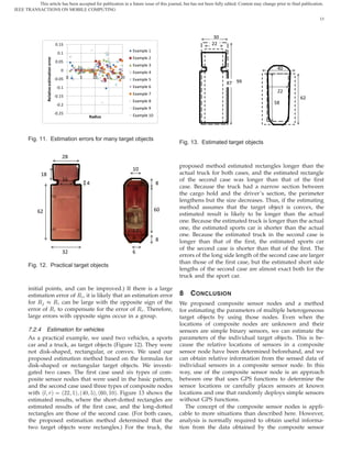
are maintained.) Figure 5 plots Á¾ averaged over every
200 measurement epochs (that is, every 2000 length unit
movement along the Ü-axis) and its total average (Á¾ 30
averaging over 2000 measurement epochs) for ´Ð Öµ 10
Distance Distance
´¿ ½µ. Although the Á¾ averaging over every 200 mea- 3 3

surement epochs changes according to the movement of
the target objects, we cannot see the difference between
the total average and that of the basic pattern (i.e., a
homogeneous Poisson process). That is, the total time
average of Á¾ under this non-homogeneous deployment
is identical to that under the basic pattern. Our proposed Fig. 6. Placement for overlap detections
estimation method uses the total time average of Á¾ and
provides us the same estimation result if Á¾ is the same.
This fact suggests that our estimation method can work
not detect multiple target objects. However, in a practical
with non-homogeneous deployment.
situation, this is not the case. We evaluated the impact
Theoretically, we do not require a homogeneous Pois-
of the overlaps of detections for the basic pattern. As
son process or homogenous density to validate the the-
shown in Figure 6, we placed three target objects, which
oretical results. As long as the average density can be
went along the Ü-axis (the bottom line) in this figure
defined over the monitored area ¨ and takes the same
without changing their relative positions. Figure 7 plots
value, Æ ´½ µ ( Æ ´¾ µ ) does not change. Thus, a
the relative errors of overlapped detections when the
doubly stochastic Poisson process, for example, is also
distance of each pair of neighbor target objects were 10
possible [11]. However, non-homogeneous density may
and 2. Due to the overlapped detections, Á¾ increased
cause a bias and additional variance for each sample.
for any ´Ð Öµ. When the distance was 10, the event in
Generally, if the average density over the route of a target
which a single sensor simultaneously detects multiple
object is equal to that over the monitored area, there is no
target objects did not occur. Thus, the total number
bias. The total average in Figure 5 is one such example.
of sensors detecting at least one target object did not
If the average density over the route of a target object
include errors. Thus, Á½ decreased for any ´Ð Öµ. (In
is not equal to that over the monitored area, should
fact, Á¾ for small Ð does not change when distance =
be defined as the average density over the route. If we
10 because the distance is large. Therefore, Á½ does not
can monitor the same target objects multiple times, the
decrease.) When the distance was 2, Á¾ increased and
ensemble average of the density over trajectories can be
the total number of sensors detecting at least one target
a definition of . Otherwise, bias may occur. In such a
object slightly decreased.
case, the results can be route dependent. An advanced
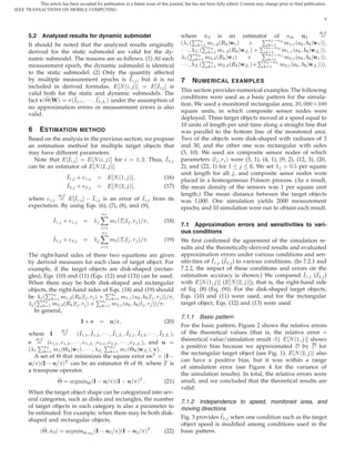
method useful for the route dependence is to estimate 7.1.6 Impacts of target objects
the average density over the route. This is for further
In addition, we investigated cases in which the target
study.
objects different from the basic pattern and are homoge-
neous. Other conditions are the same with the basic pat-
tern. We used three examples where all the target objects
3000
(l, r) = (3, 1)
were disk-shaped, and their radiuses Ê (½ ¿) were
2500 the same for each example, 3, 10, and 30, respectively.
2000 Afterwards, we used three examples where all the target
1500 objects were rectangular and all of their sides ´ µ

1000 Every 200 (½ ¿) were the same for each example, (20, 20), (10,
Total average 30), and (30, 30), respectively. The relative errors when
500
Average (basic pattern) all the target objects were disk-shaped with Ê ¿¼ and
0 those when all the target objects were rectangular with
<200 < 600 < 1000 < 1400 < 1800 ´ µ ´¿¼ ¿¼µ are shown in Figure 8. As shown in
Measurement epochs this figure, the relative errors for the disk-shaped target
objects are negligible. However, those for the rectangular
target objects can be positive or negligible. The reason of
Fig. 5. Non-homogeneous density
the positive bias is the proposed approximation uses
instead of . The relative errors for other examples are
similar.
7.1.5 Detection overlaps
In the theoretical analysis, we assumed that there are 7.2 Examples of estimation
no overlaps of detections. That is, at each measurement This subsection provides some examples of estimation.
epoch, we assume that each composite sensor node does We used a sample algorithm shown in Appendix E, but


11

7.2.1 Under various errors
0.03
Distance between target object = 10
0.02 For all the cases (the basic pattern and its modifications)
0.01 in which we evaluated in the previous subsection, we
Relative difference

0 used the proposed estimation method. As described in
-0.01 (3, 1) (4, 1) (9, 2) (12, 3) (20, 2) (22, 1) the beginning of this section, there were three target ob-
-0.02 jects (two of the objects were disk-shaped with radiuses
-0.03 of 3 and 30, and the other one was rectangular with sides
-0.04
(3, 10)) in the basic pattern.
-0.05 Number of sensors detecting
-0.06
Figure 9 plots the results. Small variations of sensed
(l, r) results have a different impact on the estimated param-
eters. The estimation for Ê¾ , the radius of the largest
0.1
disk-shaped target object, is very accurate, and there
Distance between target object = 2 is almost no errors for all cases. This is because other
0.05 target objects have nothing to do with the sensed results
Relative difference

with ´Ð Öµ ´¾¼ ¾µ ´¾¾ ½µ for any cases and the sensed
0 results with ´Ð Öµ ´¾¼ ¾µ ´¾¾ ½µ can dedicatedly be
(3, 1) (4, 1) (9, 2) (12, 3) (20, 2) (22, 1) used to estimate Ê¾ . Two other reasons are there is no
-0.05
approximation error for a disk-shaped target object and
-0.1 the approximation errors for a rectangular target object
Number of sensors detecting does not affect the largest disk-shaped target object.
-0.15 On the other hand, small variations and approximation
(l, r)
errors of sensed results cause estimation errors of the
other three parameters. This is mainly because there
Fig. 7. Relative errors due to overlap detections is an approximation error for a rectangular target ob-
ject, and the small variations can change the results
around the minimum square point. The fact is that,
for three unknown parameters, four sensed results with
0.008
0.007
E[N(1, j)]: rectangle ´Ð Öµ ´¿ ½µ ´ ½µ ´ ¾µ ´½¾ ¿µ may not be enough
E[N(2, j)]: rectangle under erroneous conditions. In total, there can be 20%
0.006
Relative error

0.005 E[N(1, j)]: disk
of estimations errors for many cases. However, overlap
0.004 E[N(2, j)]: disk
detections cause more serious estimation errors. One of
0.003
0.002
the main reasons is that they causes serious bias. Another
0.001 reason is that, due to the approximation analysis for
0 a rectangular target object, errors that give smaller Á
-0.001 (3, 1) (4, 1) (9, 2) (12, 3) (20, 2) (22, 1) increase estimation errors. For the distance of each pair
(l, r) of neighbor target object is 2, the proposed estimation
Side length of rectangles : (30, 30).
Radius of disks : 30.
method fails to detect that there are two disks and one
rectangle. It estimated as three disks. “Overlap” in this
figure corresponds to the case in which the distance of
Fig. 8. Relative errors (Three homogenous disks or three each pair of neighbor target objects is 10.
homogeneous rectangles)
7.2.2 Homogeneous target objects
When multiple target objects have similar parameter
it is not a special one. We start the estimation algorithm values, it may be difficult to estimate them. This is
with the initial values of ¢ ´½¼ ¡ ¡ ¡ ½¼µ for each pair of because it is difficult to judge whether a given set of
(Ò ÒÖ ), where ¼ Ò ÒÌ , ÒÖ ÒÌ Ò . (Eqs. (21) and composite sensor nodes is an observing parameter set.
(22) may have a local minimum in our experience. Thus, Thus, we estimated when all the three target objects have
the obtained estimates may depend on the initial values. the same parameter values: they were all disk-shaped
However, we cannot try all initial values. Therefore, we target objects with Ê ¿ ½¼ or 30, or they were all
fixed the initial values and evaluated the results.) For all rectangular target objects with ´ µ= (20, 20), (10, 30),
examples, the total number of target objects are known, or (30, 30). (The relative errors are shown in the previous
and any of the target object can be disk-shaped and subsection.)
rectangular. The number of disk-shaped target objects is Figure 10 plots the relative estimation errors. Clearly,
unknown (equivalently, the number of rectangular target the disk radius estimates are accurate. The possibility
objects is unknown) and can take any integer from 0 to of estimation for the homogeneous disk-shaped target
ÒÌ . Therefore, all examples use Eq. (22) instead of Eq. objects with Ê ¿ (½ ¿) is a unique feature for
(21). the homogeneous target objects. When Ê Ð ¾Ö , the


12

0.4

Relative estimation error
Three rectangles Three disks
b_1 = 10 0.3
*) with additional
0.2 types of composite
sensor nodes.
Overlap 0.1
a_1 = 3
Small number epochs 0
Low speed (20, 20) (10, 30) (30, 30) 3 10 30
-0.1
Different direction *
R_2 = 30
Different area -0.2
(Side 1, Side 2) (Radius)
Non-homo density
Different density R_1 = 3
Basic pattern Fig. 10. Estimation errors for multiple homogeneous
target objects
-0.8 -0.6 -0.4 -0.2 0 0.2 0.4
Relative estimation errors
7.2.3 Many target objects
It is difficult to apply this proposed method when the
number ÒÌ of target objects is large. Practically, there
Fig. 9. Relative estimation errors are two reasons. The first is that, for a fixed number
of composite sensor nodes, it is likely that a given set
of parameter values of composite sensor nodes is not
an observing parameter set when ÒÌ is large. Therefore,
-th composite sensor node cannot offer new informa- we may not be able to estimate all the parameters of
tion that is not offered by a non-composite disk-shaped the target objects. To avoid such a situation, we may
simple sensing area, although multiple non-composite
È È
need a large number of composite sensor node types.
disk-shaped sensing areas with different radiuses can The second reason is that it becomes computationally
offer Ì and Ì (See Eq.(5)). Thus, normally,
È
difficult to find the minimum square error solution.
each Ê cannot be estimated. In practice, however, when
È ÒÌ However, difficulties of such a problem that may have
½ Ì ÒÌ Ê ( Ê Ê½ Ê¾ Ê¿ ) is given,

È Ê¾ for all
È
ÒÌ local minimums with large unknown parameters are not
½ Ì is minimized at Ì and
ÒÌ Ê¾ . (The actual sensed
ÒÌ ÒÌ specific to our problem.
½ Ì
½ Ì is
È È
ÒÌ Ê¾ if there are no measurement errors.) If the sensed
We estimated the parameters of 20 target objects,
ÒÌ ¾ ÒÌ which were all disk-shaped. When estimating, we did
½ Ì is ÒÌ Ê with ½ Ì ÒÌ Ê, every target
not use the information that all the target objects are
object is disk-shaped with the radius Ê. Therefore, even
Ð ¾Ö for many , we can conclude that all
disk-shaped. To estimate the 20 target object radiuses
when Ê randomly distributed according to the uniform distribu-
the target objects are disk-shaped with the same radius. tion over the range of [1, 20] and the number Ò of disk-
As a whole, for disk-shaped homogeneous target objects, shaped target objects, we used 100 types of composite
we can accurately estimate their parameters. sensor nodes where ¼ ,Ö ¼ £ ´ · ½µ for
However, for the rectangles, the estimation accuracy ´ ½¼µ £ ½¼, Ð ¼ ¾ £ ´ · ½µ · ¾Ö . (Ð ¾Ö
for the second and third examples is poor. In particular, is at a regular interval of 0.2 from 0.2 to 20.) We used
for the second example, the proposed method did not the theoretical value of Á¾ as sensed data because
correctly estimate the number of rectangular target ob- the simulation requires so many hours. (As mentioned
jects. Therefore, we were not able to define the relative in the example of homogeneous target objects, we did
estimation error. Thus, we introduced an additional type not use Á½ for estimation because there are many types
of composite sensor node of ´Ð Öµ=(35, 2). In addition, of composite sensor nodes.) We tried 10 examples.
we did not use Á½ for estimation. This is because, as Figure 11 plots the relative errors of estimated ra-
the number of composite sensor node types increase,
Á½ does not provide any new information, but ¾
½
È diuses. (For every example, the number Ò of disk-
shaped target objects was correctly estimated. That is,
increases. Thus, Á¾ does not affect the estimation for the the estimated Ò ¾¼.) The estimation-error range was
additional composite sensor nodes. approximately between -0.1 and 0.1, except for Example
By introducing this additional type of composite sen- 10. (The estimated radiuses in Example 10 may have
sor node of ´Ð Öµ=(35, 2), the proposed method correctly shown local minimum square errors, but not global min-
estimates the number of rectangular target objects and imum square errors, because the square errors obtained
the relative estimation error can be defined and plotted. were fairly large. Thus, the results of Example 10 may
(If we use Á½ , additional types of composite sensor be dependent of the minimum-search algorithm, the
nodes are necessary.) parameters of the minimum-search algorithm, and the


13

30
0.15 22
Example 1
0.1
Example 2
Relative estimation error

0.05
Example 3
0 40
Example 4
-0.05 0 5 10 15 20
Example 5
87 99
-0.1 Example 6
Example 7
22
-0.15 62
Example 8 58
-0.2
Example 9
-0.25 Example 10
Radius

Fig. 11. Estimation errors for many target objects
Fig. 13. Estimated target objects

28
proposed method estimated rectangles longer than the
10
18 actual truck for both cases, and the estimated rectangle
16 of the second case was longer than that of the first
4 8 8
26 case. Because the truck had a narrow section between
the cargo hold and the driver’s section, the perimeter
lengthens but the size decreases. Thus, if the estimating
60 method assumes that the target object is convex, the
62 estimated result is likely to be longer than the actual
one. Because the estimated truck is longer than the actual
one, the estimated sports car is shorter than the actual
22
one. Because the estimated truck in the second case is
8 8 longer than that of the first, the estimated sports car
of the second case is shorter than that of the first. The
32 6
errors of the long side length of the second case are larger
than those of the first case, but the estimated short side
Fig. 12. Practical target objects
lengths of the second case are almost exact both for the
truck and the sport car.

initial points, and can be improved.) If there is a large
estimation error of Ê , it is likely that an estimation error 8 C ONCLUSION
for Ê Ê can be large with the opposite sign of the We proposed composite sensor nodes and a method
error of Ê to compensate for the error of Ê . Therefore, for estimating the parameters of multiple heterogeneous
large errors with opposite signs occur in a group. target objects by using those nodes. Even when the
locations of composite nodes are unknown and their
7.2.4 Estimation for vehicles sensors are simple binary sensors, we can estimate the
As a practical example, we used two vehicles, a sports parameters of the individual target objects. This is be-
car and a truck, as target objects (Figure 12). They were cause the relative locations of sensors in a composite
not disk-shaped, rectangular, or convex. We used our sensor node have been determined beforehand, and we
proposed estimation method based on the formulas for can obtain relative information from the sensed data of
disk-shaped or rectangular target objects. We investi- individual sensors in a composite sensor node. In this
gated two cases. The first case used six types of com- way, use of the composite sensor node is an approach
posite sensor nodes that were used in the basic pattern, between one that uses GPS functions to determine the
and the second case used three types of composite nodes sensor locations or carefully places sensors at known
with ´Ð Öµ ´¾¾ ½µ ´ ¼ µ ´ ¼ ½¼µ. Figure 13 shows the locations and one that randomly deploys simple sensors
estimated results, where the short-dotted rectangles are without GPS functions.
estimated results of the first case, and the long-dotted The concept of the composite sensor nodes is appli-
rectangles are those of the second case. (For both cases, cable to more situations than described here. However,
the proposed estimation method determined that the analysis is normally required to obtain useful informa-
two target objects were rectangles.) For the truck, the tion from the data obtained by the composite sensor


14

nodes. In general, more complex composite sensor nodes Young Engineer Award of the Institute of Electronics, Information and
yield more detailed information, but analysis then be- Communication Engineers (IEICE) in 1990, the Telecommunication Ad-
vancement Institute Award in 1995 and 2010, and the excellent papers
comes complicated. We will continue to develop the award of the Operations Research Society of Japan (ORSJ) in 1998.
use of these composite sensor nodes for estimating the His research interests include traffic technologies of communications
parameters of multiple target objects and will investigate systems, network architecture, and ubiquitous systems. Dr. Saito is a
fellow of IEEE, IEICE and ORSJ, and a member of IFIP WG 7.3.
other applications for which these composite sensor
nodes are useful.

R EFERENCES
[1] G. J. Pottie and W. J. Kaiser, Wireless Integrated Network Sensors,
Commun. ACM, 43, 5, pp. 51–58, May 2000.
[2] I. F. Akyildiz, W. Su, Y. Sankarasubramaniam, and E. Cayirci, A
Survey on Sensor Networks, IEEE Communications Magazine, 40,
8, pp. 102–114, 2002.
[3] B. W. Cook, S. Lanzisera, and K. S. J. Pister, SoC Issues for RF
Smart Dust, Proceedings of IEEE, 94, 6, pp. 1177–1196, June 2006.
[4] H. Saito, M. Umehira, O. Kagami, and Y. Kado, Wide Area
Ubiquitous Network: The Network Operator’s View of a Sensor Shinsuke Shimogawa graduated from Osaka University with a B.SC.
Network, IEEE Commun. Magazine, 46, 12, pp. 112–120, 2008. degree and an M.SC. degree in Mathematics. He received a Ph.D.
[5] http://robotics.eecs.berkeley.edu/˜pister/SmartDust/ degree from Kyushu University. He joined NTT in 1986 and is currently
[6] H. Saito, S. Shioda, and J. Harada, Shape and Size Estimation working at the NTT Service Integration Laboratories.
Using Stochastically Deployed Networked Sensors, IEEE SMC
2008, Singapore, 2008.
[7] P. Hall, Introduction to the Theory of Coverage Processes, John
Wiley & Sons, 1988.
[8] L. Lazos and R. Poovendran, Stochastic Coverage in Heteroge-
neous Sensor Networks, ACM Transactions on Sensor Networks,
2, 3, pp. 325–358, 2006.
[9] B. Liu and D. Towsley, A Study on the Coverage of Large-scale
Sensor Networks, First IEEE International Conference on Mobile
Ad-hoc and Sensor Systems, 2004.
[10] P. Manohar, S. S. Ram, and D. Manjunath, On the Path Coverage
by a Non-homogeneous Sensor Field, Proc. IEEE Globecom, 2006.
[11] H. Saito, K. Shimogawa, S. Shioda, and J. Harada, Shape Estima-
tion Using Networked Binary Sensors, INFOCOM 2009, 2009.
[12] H. Saito, Y. Arakawa, K. Tano, and S. Shioda, Experiments on Sadaharu Tanaka received the B.E. and M.E. degrees in communica-
Binary Sensor Networks for Estimation of Target Perimeter and tion system engineering from Chiba University, Japan, in 2008 and 2010,
Size, IEEE SECON 2009, Rome, 2009. respectively. Currently, he is with the Yahoo Japan Corporation. His
[13] H. Saito, S. Tanaka, and S. Shioda, Estimating Size and Shape of research interest includes the performance analysis of sensor networks.
Non-convex Target Object Using Networked Binary Sensors, IEEE
SUTC 2010, Newport Beach, California, USA.
[14] L. Lazos, R. Poovendran, and J. A. Ritcey, Probabilistic Detection
of Mobile Targets in Heterogeneous Sensor Networks, IPSN07,
pp. 519–528, 2007.
[15] L. A. Santalo, Integral Geometry and Geometric Probability, Sec-
´
ond edition. Cambridge University Press, Cambridge, 2004.
[16] S. Kwon and N. B. Shroff, Analysis of Shortest Path Routing for
Large Multi-hop Wireless Networks, IEEE/ACM Trans. Network-
ing, 17, 3, pp. 857–869, 2009.
[17] W. Choi and S. K. Das, A Novel Framework for Energy-
Conserving Data Gathering in Wireless Sensor Networks, INFO-
COM2005, pp. 1985–1996, 2005.
[18] D. Tian and N. Georganas, A Coverage-preserving Node Schedul- Shigeo Shioda received the B.S. degree in physics from Waseda
ing Scheme for Large Wireless Sensor Networks, First ACM University in 1986, the M.S. degree in physics from University of Tokyo
International Workshop on Wireless Sensor Networks and Ap- in 1988, and the Ph.D degree in teletraffic engineering from University
plications, pp. 32–41, 2002. of Tokyo, Tokyo, Japan, in 1998. In 1988 he joined NTT, where he
[19] F. Ye, G. Zhong, S. Lu, and L. Zhang, Peas: A Robust Energy was engaged in research on measurements, dimensioning and controls
Conserving Protocol for Long-lived Sensor Networks, Proc. IEEE for ATM-based networks. Since March 2001, he has been with the
ICDCS, 2003. graduate school of engineering, Chiba University, Japan, where he is
[20] S. Shakkottai, R. Srikant, and N. Shroff, Unreliable Sensor Grids: now Professor. His research interests are in the field of performance
Coverage, Connectivity and Diameter, Proc. IEEE INFOCOM, evaluation of wireless networks, P2P systems, queueing theory, and
2003. complex networks. Prof. Shioda is a member of the ACM, the IEEE,
[21] H. Saito, S. Tanaka, and S. Shioda, Stochastic Geometric Filter and the IEICE, and the Operation Research Society of Japan.
its Application, submitted for publication.

Hiroshi Saito graduated from the University of Tokyo with a B.E.
degree in Mathematical Engineering in 1981, an M.E. degree in Control
Engineering in 1983 and received Dr.Eng. in Teletraffic Engineering
in 1992. He joined NTT in 1983. He is currently an Executive Re-
search Engineer at NTT Service Integration Labs. He received the

Estimating Parameters of Multiple Heterogeneous Target Objects Using Composite Sensor Nodes

More Related Content

What's hot

Viewers also liked

Similar to Estimating Parameters of Multiple Heterogeneous Target Objects Using Composite Sensor Nodes

More from ambitlick

Recently uploaded

Estimating Parameters of Multiple Heterogeneous Target Objects Using Composite Sensor Nodes