Download to read offline
![7
We also experienced very strong echoes in the room,
because of its cement construction and solid wood
lab benches. Working in an environment with reduced
echoes would probably have yielded better results. This
was evident during late nights in the lab when people
working in the ASAP room and janitorial staff would
peek into the room to find the very loud noise echoing
throughout the HSH.
On the software side, we experienced difficulties get-
ting the bandwidth we desired over RTDX. I had also
seen poor RTDX performance before, when sending data
from a PC to the DSK during the cosine generation lab.
There are several possible causes of this: One is that
we only send a few bytes at a time, but do it dozens
of times per second. Recommendations we found online
suggested that filling the RTDX queue and sending large
packets of data is the fastest way to send data.
Another likely cause is our DSK boards. We read a
mailing list correspondence between someone who is
familiar with this family of DSKs and a hapless hobbyist
having similar issues. The “expert” claimed that there
is obfuscation hardware on the DSK boards introduced
by Spectrum Digital that slows down RTDX communi-
cation. It was mentioned that a possible workaround is
using the JTAG connector on the DSK board, but the
hardware required for this is not readily available (and
the JTAG port is blocked by the DSP_AUDIO_4). We
looked at high-speed RTDX, but it is not supported on
this platform.
IX. CONCLUSION
Although we did not meet our initial specifications,
our project was still somewhat successful. We were able
to implement a working beamforming system, and most
of the problems we encountered were limitations of our
equiment which were not under our control.
REFERENCES
[1] M. Brandstein and D. Ward, eds., Microphone Arrays: Signal Pro-
cessing Techniques and Applications. Berlin, Germany: Springer,
2001.
[2] J. Benesty, J. Chen, and Y. Huang, Microphone Array Signal
Processing. Berlin, Germany: Springer, 2008.
[3] J. Chen, L. Yip, J. Elson, H. Wang, D. Maniezzo, R. Hudson,
K. Yao, and D. Estrin, “Coherent Acoustic Array Processing and
Localization on Wireless Sensor Networks,” Proceedings of the
IEEE, vol. 91, no. 8, pp. 1154–1162, 2003.
[4] J. C. Chen, K. Yao, and R. E. Hudson, “Acoustic Source Localiza-
tion and Beamforming: Theory and Practice,” EURASIP Journal
on Applied Signal Processing, pp. 359–370, 2003.
[5] T. Haynes, “A primer on digital beamforming,” Spectrum Signal
Processing, 1998.
[6] W. Herbordt and W. Kellermann, “Adaptive Beamforming for Au-
dio Signal Acquisition,” Adaptive Signal Processing: Applications
to Real-World Problems, pp. 155–196, 2003.
[7] R. A. Kennedy, T. D. Abhayapala, and D. B. Ward, “Broadband
nearfield beamforming using a radial beampattern transformation,”
IEEE Transactions on Signal Processing, vol. 46, no. 8, pp. 2147–
2156, 1998.
[8] R. J. Lustberg, “Acoustic Beamforming Using Microphone Ar-
rays,” Master’s thesis, Massachusetts Institute of Technology,
Cambridge, MA, June 1993.
[9] N. Mitianoudis and M. E. Davies, “Using Beamforming in the
Audio Source Separation Problem,” in 7th Int Symp on Signal
Processing and its Applications, no. 2, 2003.](https://image.slidesharecdn.com/dspfinalreport-161010100610/85/Dsp-final-report-9-320.jpg)
![10
1 function [outputSignal] = delay(inputSignal, time, Fs)
2 % DELAY - Simulates a delay in a discrete time signal
3 %
4 % USAGE:
5 % outputSignal = delay(inputSignal, time, Fs)
6 %
7 % INPUT:
8 % inputSignal - DT signal to operate on
9 % time - Time delay to use
10 % Fs - Sample rate
11
12 if(time < 0)
13 error(’Time delay must be positive’);
14 end
15
16 outputSignal = [zeros(1, floor(time * Fs)), inputSignal];
17
18 % Crop the output signal to the length of the input signal
19 outputSignal = outputSignal(1:length(inputSignal));](https://image.slidesharecdn.com/dspfinalreport-161010100610/85/Dsp-final-report-12-320.jpg)
![12
52
53
54 % Distance from the source to the mic
55 prop1Distance = hypot(source1LocX - micLocX, source1LocY - micLocY);
56 prop2Distance = hypot(source2LocX - micLocX, source2LocY - micLocY);
57
58 time1Delay = prop1Distance/speedOfSound;
59 time2Delay = prop2Distance/speedOfSound;
60
61 % Create some of the signal
62 soundTime = 0:1/Fs:.125;
63
64 source1Signal = sin(2 * pi * source1Freq * soundTime);
65 source2Signal = sin(2 * pi * source2Freq * soundTime);
66
67 % Delay it by the propagation delay for each mic
68 for ii = 1:numMicrophones
69 received(ii,:) = delay(source1Signal, time1Delay(ii), Fs)...
70 + delay(source2Signal, time2Delay(ii), Fs);
71 end
72
73
74 % Direct the beam towards a location of interest
75 angleWanted = 45; % Degrees (for simplicity)
76 angleToDelay = angleWanted * pi/180; % Convert to radian
77
78 % We want to take the fft of the signal only after everymicrophone is
79 % getting all of the data from all sources
80 deadAirTime = (max([time1Delay, time2Delay]));
81 deadAirSamples = deadAirTime * Fs;
82 endOfCapture = length(received(1,:));
83
84 % Start off with an empty matrix
85 formedBeam = zeros(1, max(length(received)));
86
87 % For each microphone add together the sound received
88 for jj = 1:numMicrophones
89 formedBeam = formedBeam + ...
90 delay(received(jj,:), + timeSpacing*sin(angleToDelay) * (jj-1), Fs);
91 end
92
93 % Get the PSD object using a modified covariance
94 beamPSD = psd(spectrum.mcov, formedBeam,’Fs’,44100);
95 % Get the magnitude of the PSD
96 formedSpectrum = abs(fft(formedBeam));
97 % The fft sample # needs to be scaled to get frequency
98 fftScaleFactor = Fs/numel(formedSpectrum);
99
100 % The frequencies we are interested in are:
101 % Right now this is optimized for sources between 100 and 500 Hz
102 %fmin = 0; % Hz
103 %fmax = 600;% Hz
104
105 % Plot the PSD of the received signal](https://image.slidesharecdn.com/dspfinalreport-161010100610/85/Dsp-final-report-14-320.jpg)
![14
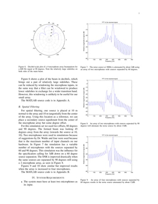
APPENDIX C
C CODE FOR MAIN PROCESSING LOOP
1
2 void processing(){
3 Int16 twoMicSamples[2];
4
5 Int32 totalPower; // Total power for the data block, sent to the PC
6 Int16 tempPower; // Value used to hold the value to be squared and added
7 Int16 printCount; // Used to keep track of the number of loops since we last sent data
8 unsigned char powerToSend;
9
10 Int8 firstLocalizationLoop; // Whether this is our first loop in localization mode
11 Int8 delay; // Delay amount for localization mode
12
13 QUE_McBSP_Msg tx_msg,rx_msg;
14 int i = 0; // Used to iterate through samples
15
16 RTDX_enableOutput( &dataChan );
17
18 while(1){
19
20 SEM_pend(&SEM_McBSP_RX,SYS_FOREVER);
21
22 // Get the input data array and output array
23 tx_msg = QUE_get(&QUE_McBSP_Free);
24 rx_msg = QUE_get(&QUE_McBSP_RX);
25
26 // Spatial filter mode
27
28 // Localization mode
29 if(firstLocalizationLoop){
30 delay = DELAYMIN;
31 firstLocalizationLoop = FALSE;
32 }
33 else{
34 delay++;
35 if(delay > DELAYMAX){
36 delay = DELAYMIN;
37 }
38 }
39
40 // Process the data here
41 /* MIC1R data[0]
42 * MIC1L data[1]
43 * MIC0R data[2]
44 * MIC0L data[3]
45 *
46 * OUT1 Right - data[0]
47 * OUT1 Left - data[1]
48 * OUT0 Right - data[2]
49 * OUT0 Left - data[3]
50 */
51](https://image.slidesharecdn.com/dspfinalreport-161010100610/85/Dsp-final-report-16-320.jpg)
![15
52 totalPower = 0;
53
54 for(i=0; i<QUE_McBSP_LEN; i++){
55
56 // Put the array elements in order
57 twoMicSamples[0] = *(rx_msg->data + i*4 + 2);
58 twoMicSamples[1] = *(rx_msg->data + i*4 + 3);
59
60 tx_msg->data[i*4] = 0;
61 tx_msg->data[i*4 + 1] = 0;
62 tx_msg->data[i*4 + 2] = sum(twoMicSamples, delay);
63 tx_msg->data[i*4 + 3] = 0;](https://image.slidesharecdn.com/dspfinalreport-161010100610/85/Dsp-final-report-17-320.jpg)
![16
APPENDIX D
C CODE FOR SUMMING DELAYS
Listing 1. sum.h
1 #ifndef _SUM_H_BFORM_
2 #define _SUM_H_BFORM_
3 extern Int16 sum(Int16* newSamples, int delay);
4 #endif
Listing 2. sum.c
1
2 #include <std.h>
3
4 #include "definitions.h"
5 #include "calcDelay.h"
6
7 /* newSamples is an array with each of the four samples.
8 * delayIncrement is the amount to delay each microphone by, in samples.
9 * This function returns a "beamed" sample. */
10 Int16 sum(Int16* newSamples, int delayIncrement){
11 static int currInput = 0; // Buffer index of current input
12 int delays[NUMMICS]; // Amount to delay each microphone by
13 int mic = 0; // Used as we iterate through the mics
14 int rolloverIndex;
15 Int16 output = 0;
16 static Int16 sampleBuffer[NUMMICS][MAXSAMPLEDIFF];
17
18 // Calculate samples to delay for each mic
19 // TODO: Only do this once
20 calcDelay(delayIncrement, delays);
21
22 // We used to count backwards - was there a good reason?
23 currInput++; // Move one space forward in the buffer
24
25 // Don’t run off the end of the array
26 if(currInput >= MAXSAMPLEDIFF){
27 currInput = 0;
28 }
29
30 // Store new samples into sampleBuffer
31 for(mic=0; mic < NUMMICS; mic++){
32 // Divide by the number of microphones so it doesn’t overflow
33 // when we add them
34 sampleBuffer[mic][currInput] = newSamples[mic]/NUMMICS;
35 }
36
37 // For each mic add the delayed input to the current output
38 for(mic=0; mic < NUMMICS; mic++){
39 if(currInput - delays[mic] >= 0){// Index properly?
40 output += sampleBuffer[mic][currInput - delays[mic]];
41 }
42 else{
43 // The delay index is below 0, so add the length of the array
44 // to keep it in bounds](https://image.slidesharecdn.com/dspfinalreport-161010100610/85/Dsp-final-report-18-320.jpg)
![17
45 rolloverIndex = MAXSAMPLEDIFF + (currInput - delays[mic]);
46 output += sampleBuffer[mic][rolloverIndex];
47 }
48 }
49
50 return output;
51
52 }
APPENDIX E
C CODE FOR CALCULATING DELAYS
Listing 3. calcDelay.h
1 #ifndef _CALC_DELAY_H_
2 #define _CALC_DELAY_H_
3 extern void calcDelay(int delayInSamples, int* delays);
4 #endif
Listing 4. calcDelay.c
1 /* calcDelay
2 * Accepts delays in samples as an integer
3 * and returns a pointer to an array of delays
4 * for each microphone.
5 *
6 * Date: 9 March 2010
7 */
8
9 #include "definitions.h"
10
11 void calcDelay(int delayInSamples, int* delays){
12 int mic = 0;
13 if(delayInSamples > 0){
14 for(mic=0; mic < NUMMICS; mic++){
15 delays[mic] = delayInSamples*mic;
16 }
17 }
18 else{
19 for(mic=0; mic < NUMMICS; mic++){
20 delays[mic] = delayInSamples*(mic-(NUMMICS-1));
21 }
22 }
23 }
APPENDIX F
JAVA CODE - MAIN
Listing 5. MainWindow.java
1 /* MainWindow.java - Java class which constructs the main GUI window
2 * for the project, and sets up communication with the DSK. It also
3 * contains the main() method.
4 *
5 * Author: Steven Bell and Nathan West
6 * Date: 9 March 2010
7 * $LastChangedBy$
8 * $LastChangedDate$](https://image.slidesharecdn.com/dspfinalreport-161010100610/85/Dsp-final-report-19-320.jpg)
![18
9 */
10
11 package beamformer;
12
13 import java.awt.*; // GUI Libraries
14
15 import javax.swing.*;
16
17 public class MainWindow
18 {
19 JFrame window;
20 DisplayPanel display;
21 ControlPanel controls;
22 static Beamformer beamer;
23
24 MainWindow()
25 {
26 beamer = new Beamformer();
27
28 window = new JFrame("Acoustic Beamforming GUI");
29 window.setDefaultCloseOperation(WindowConstants.EXIT_ON_CLOSE);
30 window.getContentPane().setLayout(new BoxLayout(window.getContentPane(), BoxLayout.LINE
31
32 display = new DisplayPanel();
33 display.setPreferredSize(new Dimension(500,500));
34 display.setAlignmentY(Component.TOP_ALIGNMENT);
35 window.add(display);
36
37 controls = new ControlPanel();
38 controls.setAlignmentY(Component.TOP_ALIGNMENT);
39 window.add(controls);
40
41 window.pack();
42 window.setVisible(true);
43
44 beamer.start();
45 }
46
47 public static void main(String[] args)
48 {
49 MainWindow w = new MainWindow();
50 while(true){
51 beamer.update();
52 w.display.updatePower(beamer.getPower());
53 }
54 }
55 }
APPENDIX G
JAVA CODE FOR BEAMFORMER COMMUNICATION
Listing 6. Beamformer.java
1 /* Beamformer.java - Java class which interacts with the DSK board
2 * using RTDX.
3 *](https://image.slidesharecdn.com/dspfinalreport-161010100610/85/Dsp-final-report-20-320.jpg)
![19
4 * Author: Steven Bell and Nathan West
5 * Date: 11 April 2010
6 * $LastChangedBy$
7 * $LastChangedDate$
8 */
9
10 package beamformer;
11
12 //Import the DSS packages
13 import com.ti.ccstudio.scripting.environment.*;
14 import com.ti.debug.engine.scripting.*;
15
16 public class Beamformer {
17
18 DebugServer debugServer;
19 DebugSession debugSession;
20
21 RTDXInputStream inStream;
22
23 int[] mPowerValues;
24
25 public Beamformer() {
26 mPowerValues = new int[67]; // TODO: Change to numBeams
27
28 ScriptingEnvironment env = ScriptingEnvironment.instance();
29 debugServer = null;
30 debugSession = null;
31
32 try
33 {
34 // Get the Debug Server and start a Debug Session
35 debugServer = (DebugServer) env.getServer("DebugServer.1");
36 debugServer.setConfig("Z:/2010_Spring/dsp/codecomposer_workspace/dsp_project_trunk/ds
37 debugSession = debugServer.openSession(".*");
38
39 // Connect to the target
40 debugSession.target.connect();
41 System.out.println("Connected to target.");
42
43 // Load the program
44 debugSession.memory.loadProgram("Z:/2010_Spring/dsp/codecomposer_workspace/dsp_projec
45 System.out.println("Program loaded.");
46
47 // Get the RTDX server
48 RTDXServer commServer = (RTDXServer)env.getServer("RTDXServer.1");
49 System.out.println("RTDX server opened.");
50
51 RTDXSession commSession = commServer.openSession(debugSession);
52
53 // Set up the RTDX input channel
54 inStream = new RTDXInputStream(commSession, "dataChan");
55 inStream.enable();
56 }
57 catch (Exception e)](https://image.slidesharecdn.com/dspfinalreport-161010100610/85/Dsp-final-report-21-320.jpg)
![20
58 {
59 System.out.println(e.toString());
60 }
61 }
62
63 public void start()
64 {
65 // Start running the program on the DSK
66 try{
67 debugSession.target.restart();
68 System.out.println("Target restarted.");
69 debugSession.target.runAsynch();
70 System.out.println("Program running....");
71 Thread.currentThread().sleep(1000); // Wait a second for the program to run
72 }
73 catch (Exception e)
74 {
75 System.out.println(e.toString());
76 }
77 }
78
79 public void stop()
80 {
81 // Stop running the program on the DSK
82 try{
83 debugSession.target.halt();
84 System.out.println("Program halted.");
85 }
86 catch (Exception e)
87 {
88 System.out.println(e.toString());
89 }
90
91 }
92
93 public void setMode()
94 {
95
96 }
97
98 public void setNumBeams()
99 {
100
101 }
102
103 public void update(){
104 try{
105 // Read some bytes
106 byte[] power = new byte[1];
107 byte[] delay = new byte[1];
108
109 inStream.read(delay, 0, 1, 0); // Read one byte, wait indefinitely for it
110 inStream.read(power, 0, 1, 0); // Read one byte, wait indefinitely for it
111](https://image.slidesharecdn.com/dspfinalreport-161010100610/85/Dsp-final-report-22-320.jpg)
![21
112 int intPower = power[0] & 0xFF; // Convert to int value from unsigned byte
113
114 mPowerValues[delay[0] + 33] = intPower; // Save them
115
116 System.out.println("D:" + (int)delay[0] + " P: " + intPower);
117 }
118 catch (Exception e)
119 {
120 System.out.println(e.toString());
121 }
122 } // END update()
123
124 public int[] getPower()
125 {
126 return mPowerValues;
127 }
128
129 /*
130 public int[] getDelays()
131 {
132 return int
133 }*/
134
135 } // END class
APPENDIX H
JAVA CODE FOR BEAM DISPLAY
Listing 7. DisplayPanel.java
1 /* DisplayPanel.java - Java class which creates a canvas to draw the
2 * beamformer output on and handles the drawing.
3 *
4 * Author: Steven Bell and Nathan West
5 * Date: 9 March 2010
6 * $LastChangedBy$
7 * $LastChangedDate$
8 */
9
10 package beamformer;
11
12 import java.awt.*; // GUI Libraries
13 import javax.swing.*;
14 import java.lang.Math;
15
16 public class DisplayPanel extends JPanel
17 {
18
19 int mDelay[];// = {-3, -2, -1, 0, 1, 2, 3};
20 double mPower[];// = {0, .25, .5, 1, .5, .25, 0};
21 int mNumPoints = 67;
22
23 double mSpacing = 33;
24
25 DisplayPanel()
26 {](https://image.slidesharecdn.com/dspfinalreport-161010100610/85/Dsp-final-report-23-320.jpg)
![22
27 mDelay = new int[mNumPoints];
28 mPower = new double[mNumPoints];
29
30 for(int i = 0; i < mNumPoints; i++){
31 mDelay[i] = i - 33;
32 mPower[i] = .5;
33 }
34 }
35
36 void updatePower(int[] newPower)
37 {
38 for(int i = 0; i < mNumPoints; i++)
39 {
40 mPower[i] = (double)newPower[i] / 255;
41 if(mPower[i] > 1){
42 mPower[i] = 1;
43 }
44 }
45 this.repaint();
46 }
47
48 static final int FIGURE_PADDING = 10;
49
50 // Overrides paintComponent from JPanel
51 protected void paintComponent(Graphics g)
52 {
53 super.paintComponent(g);
54
55 Graphics2D g2d = (Graphics2D)g; // Cast to a Graphics2D so we can do more advanced pain
56 g2d.setRenderingHint(RenderingHints.KEY_ANTIALIASING, RenderingHints.VALUE_ANTIALIAS_ON
57
58 // Determine the maximum radius we can use. It will either be half
59 // of the width, or the full height (since we do a semicircular plot).
60 int maxRadius = this.getWidth()/2;
61 if(maxRadius > this.getHeight()){
62 maxRadius = this.getHeight();
63 }
64 maxRadius = maxRadius - FIGURE_PADDING;
65
66 // Pick our center point
67 int centerX = this.getWidth() / 2;
68 int centerY = this.getHeight()-(this.getHeight() - maxRadius) / 2;
69
70 // Calculate all of the points
71 int[] px = new int[mNumPoints];
72 int[] py = new int[mNumPoints];
73
74 for(int i = 0; i < mNumPoints; i++)
75 {
76 double angle = delayToAngle(mDelay[i]);
77 px[i] = centerX - (int)(maxRadius * mPower[i] * Math.sin(angle));
78 py[i] = centerY - (int)(maxRadius * mPower[i] * Math.cos(angle));
79 }
80](https://image.slidesharecdn.com/dspfinalreport-161010100610/85/Dsp-final-report-24-320.jpg)
![23
81 g2d.setPaint(Color.BLUE);
82 g2d.drawPolygon(px, py, mNumPoints);
83
84 // Draw the outline of the display, so we have some context
85 g2d.setPaint(Color.BLACK);
86 float[] dash = {5, 4};
87 g2d.setStroke(new BasicStroke((float).5, BasicStroke.CAP_BUTT, BasicStroke.JOIN_MITER,
88 g2d.drawLine(10, centerY, this.getWidth() - 10, centerY);
89 g2d.drawArc(10, (this.getHeight() - maxRadius) / 2, 2*maxRadius, 2*maxRadius, 0, 180);
90 }
91
92 // Takes a delay and converts it to the equivalent in radians
93 private double delayToAngle(int delay)
94 {
95 return(Math.PI/2 - Math.acos(delay/mSpacing));
96 }
97
98 // Takes an angle in radians (-pi/2 to +pi/2) and converts it to a delay
99 private int angleToDelay(double angle)
100 {
101 return(int)(mSpacing * Math.cos(angle + Math.PI/2));
102 }
103 }](https://image.slidesharecdn.com/dspfinalreport-161010100610/85/Dsp-final-report-25-320.jpg)

This document describes the design and implementation of an acoustic beamforming system using a microphone array and the TDS3230 DSK board. It discusses the theory of delay-and-sum beamforming and the design of the microphone array. Simulations were conducted in MATLAB to test source localization and spatial filtering capabilities. The system requirements and overall design are then described, including the hardware, DSP software, and GUI interface. Tests were planned to evaluate source localization accuracy and the ability to filter out noise sources located at different angles.