1. 2015 Noah Beilin December 11, 2015
Abstract
Artificial or natural random noise surrounds us
everyday. Whether it is a crowded school lobby
where a variety of peoples' voices come
together to make random non-sense, or even on
a busy highway that is heavily impacted by
traffic, these 'ambient' noises are a reality many
of us have to face. Fortunately, many of us have
the ability to 'filter' out some of this irrelevant
noise in our own minds by simply paying
attention to something else more meaningful.
This however, is unfortunately not the case for
many of our audio recording/ playback devices
that are used on a daily basis by almost every
consumer. In fact, depending on the sampling
rate of the device, most of the irrelevant noise
will get recorded or played back from and to us
without any desire. This is obviously a big issue
for many of us who use cellular or VoIP devices
throughout the day. The random noise that
surrounds us can obviously not be 'turned
down', and it will be distractingly be included
in our electronic conversations. Despite the fact
that our external environment isn't so easy to
control however, our recording and playback
devices are. That being said, some of these
issues we face on a day-to-day base can be
fixed by modifying our devices to 'work' around
these annoying noises.
To do this though, it is necessary to understand
what 'noise' is, how it can be manipulated, and
its properties. From that, we can apply our
understanding of it in order to modify the
software and hardware of our devices to help
tune out these noises for our hearing pleasure.
White Noise
White noise is a signal that is composed of a
uniform distribution of sinusoids of equally
weighted magnitudes, but different periodic
values (ideally: f = 0 - ∞ Hz). To many of us,
this can be pictured as the static noise we hear,
or the white scrambled image we see when a a
corrupt video feed comes into an old school
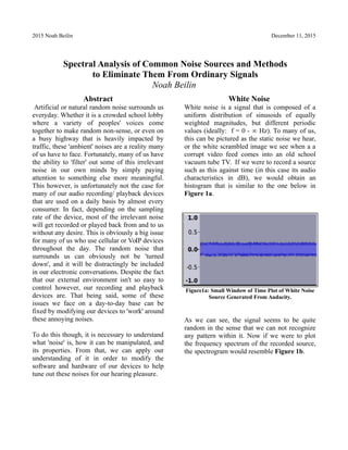
vacuum tube TV. If we were to record a source
such as this against time (in this case its audio
characteristics in dB), we would obtain an
histogram that is similar to the one below in
Figure 1a.
Figure1a: Small Window of Time Plot of White Noise
Source Generated From Audacity.
As we can see, the signal seems to be quite
random in the sense that we can not recognize
any pattern within it. Now if we were to plot
the frequency spectrum of the recorded source,
the spectrogram would resemble Figure 1b.
Spectral Analysis of Common Noise Sources and Methods
to Eliminate Them From Ordinary Signals
Noah Beilin

2. 2015 Noah Beilin December 11, 2015
Figure 1b: Spectrogram of White Noise Source
Measured from 0Hz to 8000Hz
The spectrogram displays the density (or
magnitude) of each frequency component of a
signal. As stated before, white noise ideally
consists of an equal amount of every frequency
from 0 to infinite. If we analyze the above
figure above, we can clearly see that the signal
generated consists of a distribution of frequency
values that is quite close to being uniform. This
pattern would keep its integrity at higher
frequencies as well. If this were to come from
an ideal white noise source however
(impossible to create in real world), we would
get a straight line centered at a single dB value.
What is interesting, is the fact that everyday
common sources of noise we hear, resembles
some characteristics of white noise. For an
example, Figure 2a is a time plot of a recording
taken in close proximate to a 'noisy' power
plant on CalPoly's campus. The device that
recorded it was a standard smart phone that
sampled the audio at 16kHz.
Window of Noise Recorded Nearby Power Plant.
Sampled at 16kHz using Android OS based Smart
Phone.
Although it is hard to analyze signals such as
this from a time series, we can at least observe
that the white noise source and the power plant
both have random characteristics to it. Now lets
look at the power plant's spectrogram as seen in
Figure 2b.
Figure 2b: Spectrogram of Recorded Power Plant
Noise. N = 32000
Although the power plant's spectrogram has
differences to the characteristic's of the white
noise's, there definitely are a handful of
similarities. First off, just by looking at the
Figure 1b and Figure 2b, we can see that both
noise sources do in fact consist of a wide range
of frequency values. Next, we can see how
much of each wave form is periodic by
autocorrelating both the white noise source
Figure 3a, and the power plant source Figure
3b.
Figure 3a: autocorrelation plot of power plant signal.
Figure 3b: autocorrelation plot of white noise source

3. 2015 Noah Beilin December 11, 2015
As we can see from both figures, the white
noise source and the power plant noise
autocorrelation factor stays at zero. This shows
that both signals are aperiodic, or quite random.
From this we can conclude that many
environmental noises share similarities to white
noise, and thus are random and aperiodic as
well.
Other Noises
A couple of other common noises on campus
were recorded. Their spectrograms are shown
below.
Figure 4a: Spectrogram of Medium-Sized Household
fan located in Kennedy Library. N = 32000
Figure 4b: Spectrogram of Car Garage during Non
Rush Hour time frame. N = 32000
Looking at the two previous figures. We again,
can see a common pattern where environmental
noise pollution consists of random frequencies.
The main difference between all of the noise
sources we analyzed though, is the fact that the
magnitudes of the frequency densities vary from
each other across each spectrum.
Speech
Now, we would like to analyze the signal
composition of a standard greeting recorded
into the same device at the same sampling rate.
In Figure 5a, we can see a spectrogram of an
audio clip of me saying “hello” multiple time
(in a room with no noise pollution). Unlike the
noises that were recorded from the campus
locations, this one does not nearly have as wide
as of a range of frequency values as the other
noisy signals.
Figure 5a: Spectrogram of Recorded Voice Greeting
in Isolated Environment. N = 32000
With this observation, we can assume that most
common speech phrases consist of a much
narrower frequency spectrum than
environmental noise sources. With that in mind,
it would be ideal if there was some how a way
to cut-off the unnecessary frequencies (Those
that are not a part of the speech) that partially
compose the interfering noise sources when
recording/ playing back audio to and from our
device.

4. 2015 Noah Beilin December 11, 2015
Analog/ Digital Filtering
The application of a filter to an un-isolated
speech signal (i.e. one in combination with a
noisy source) can help eliminate some of the
unwanted noise in your speech. Take a look at
Figure 6. This is simply the spectrogram of the
power plant noise mixed in with the “hello”
speech greeting from the previous figures. As
we can see, the spectrogram shows us that
much of the noisy signal did not get effected
near higher frequencies. We can also see in the
previous speech figure, that most of the
frequency density was higher in the 440Hz-
1kHz range. This aids the fact why the Figure 6
has a larger density value in this range.
Figure 6: Spectrogram of Power Plant Noise Mixed
with “Hello” signal.
Now if we go ahead and apply a low-pass filter
with a cutoff frequency at 1000Hz (with a 12dB
roll-off) through audacity, we can get the
filtered signal as seen in Figure 7.
Although there are still unwanted elements
present in the reconstructed signal, we can see
that it resembles the original “hello” much
closer than that shown in Figure 6. What is
even more interesting, is the fact that the
“Hello” phrase can be heard much more clearly
when the filter is applied to the mixed track.
This is because it muffles out the higher
frequency noises, and keeps the lower
frequency range (which is beneficial to me
since I have a deep voice).
With this analysis, we can conclude that the
application of a digital/ analog filter to
incoming/ outgoing audio signal can
reconstruct the sought main signal with less
noise.
This leads to another conclusion that the type of
filter to apply to each signal will depend on the
location the signal is created (I.e the
characteristics of the noise elements that
surround it), and the characteristics of the
signal itself (i.e. high/ low-pitch voice).
We can utilize a useful tool known as cross
correlation in order to determine the type of
filter to apply to the incoming signals.
Cross Correlating Filter Transfer
Functions and Signal Characteristics
In signal processing, cross-correlation is a
measure of similarity of two series as a function
of the lag of one relative to the other. In order to
get a sense of how this can be used for this
purpose, we go ahead and correlate the data of
the spectrogram of the “hello” signal with the
transfer characteristics of a low-pass filter with
1000Hz cut-off (12db roll-out). Both
Spectrograms are now padded with a sampling
period of N = 128 (as seen below in figure 8a
and 8b). The data from the 126 samples of both
spectrum are then exported into Libre Office
Calc, where a column is designated for each
data series (sample data window figure 9).

5. 2015 Noah Beilin December 11, 2015
Figure 8a: Transfer Characteristics of Low-Pass
Filter. N = 128.
Figure 8b: Spectrogram of “Hello” Signal. N = 128
Figure 9: Sample Window of Data Series used in
Spread Sheet Calculation
The two columns ares the correlated with one
another using the following function:
correl(A1:A125, B1:B125)
The following is the result that was given by
the spreadsheet program:
0.9186
Knowing that when the cross correlation is
closer to unity, the two series of data are more
closely correlated as a result.
With that previous statement in mind, we can
take any speech signal's spectrogram and cross
correlate it a variety of different types of filters'
transfer characteristic plots. This means that in
some situations, a band pass filter would be
ideal if its correlation to the original speech
signal is closer to one instead.
Along with that, we could also see what types
of filters attenuate the noise component of a
signal the best by trying to achieve a cross
correlation closer to negative 1. In other words,
If we wanted to attenuate the noise coming
from Car Garage, it would be ideal to apply a
high-pass cutoff filter around 4Khz.
To prove this, the same method was applied
above in order to cross correlate a high-pass
filter with the car garage noise. The result is
listed below:
-0.9146
As we can see by the almost negative unity
value, the 4Khz HP filter would work well in
filtering out that nonsense noise.
Conclusion
As you may know, there are many
computational algorithms can model statistical
analysis methods (such as cross correlation) at a
software and hardware level. Some of the
algorithms are used to create many useful
applications in signal processing, especially
with the implementation of adaptive filters
Adaptive filters are computational devices that
attempt to model the relationship between two
signals (1). These computational algorithms
have been used previously to create adaptive
noise filtering applications, and even
automation. Although the math itself does
require a broader, more theoretical
125 -35.976479 125 -33.828056
250 -36.161873 250 -34.038429
375 -31.271317 375 -34.204353
500 -31.927086 500 -34.543018
625 -41.580437 625 -34.877216
750 -46.536419 750 -35.705086

6. 2015 Noah Beilin December 11, 2015
understanding, we can see that mathematical
models can be created in order to achieve
proper noise filtration. It is just a matter of how
you apply the mathematical model in a real
world application. That being said, the notion
of cross correlation can be applied to adaptive
noise filtration. One could possibly write a
program that run a cross correlation algorithm
amongst the desired input signal with a series of
different transfer characteristics of filters,
compare all of the ratios, and then pick out the
filter with the highest value to apply to the
incoming signal.
Reference
(1) Hayes, Monson H. (1996). Statistical
Digital Signal Processing and Modeling. Wiley.