This document describes Dremel, an interactive query system for analyzing large nested datasets. Dremel uses a multi-level execution tree to parallelize queries across thousands of CPUs. It stores nested data in a novel columnar format that improves performance by only reading relevant columns from storage. Dremel has been in production at Google since 2006 and is used by thousands of users to interactively analyze datasets containing trillions of records.

1. Dremel: Interactive Analysis of Web-Scale Datasets
Sergey Melnik, Andrey Gubarev, Jing Jing Long, Geoffrey Romer,
Shiva Shivakumar, Matt Tolton, Theo Vassilakis
Google, Inc.
{melnik,andrey,jlong,gromer,shiva,mtolton,theov}@google.com
ABSTRACT
Dremel is a scalable, interactive ad-hoc query system for analy-
sis of read-only nested data. By combining multi-level execution
trees and columnar data layout, it is capable of running aggrega-
tion queries over trillion-row tables in seconds. The system scales
to thousands of CPUs and petabytes of data, and has thousands
of users at Google. In this paper, we describe the architecture
and implementation of Dremel, and explain how it complements
MapReduce-based computing. We present a novel columnar stor-
age representation for nested records and discuss experiments on
few-thousand node instances of the system.
1. INTRODUCTION
Large-scale analytical data processing has become widespread in
web companies and across industries, not least due to low-cost
storage that enabled collecting vast amounts of business-critical
data. Putting this data at the fingertips of analysts and engineers
has grown increasingly important; interactive response times of-
ten make a qualitative difference in data exploration, monitor-
ing, online customer support, rapid prototyping, debugging of data
pipelines, and other tasks.
Performing interactive data analysis at scale demands a high de-
gree of parallelism. For example, reading one terabyte of com-
pressed data in one second using today’s commodity disks would
require tens of thousands of disks. Similarly, CPU-intensive
queries may need to run on thousands of cores to complete within
seconds. At Google, massively parallel computing is done using
shared clusters of commodity machines [5]. A cluster typically
hosts a multitude of distributed applications that share resources,
have widely varying workloads, and run on machines with different
hardware parameters. An individual worker in a distributed appli-
cation may take much longer to execute a given task than others,
or may never complete due to failures or preemption by the cluster
management system. Hence, dealing with stragglers and failures is
essential for achieving fast execution and fault tolerance [10].
The data used in web and scientific computing is often non-
relational. Hence, a flexible data model is essential in these do-
mains. Data structures used in programming languages, messages
Permission to make digital or hard copies of all or part of this work for
personal or classroom use is granted without fee provided that copies are
not made or distributed for profit or commercial advantage and that copies
bear this notice and the full citation on the first page. To copy otherwise, to
republish, to post on servers or to redistribute to lists, requires prior specific
permission and/or a fee. Articles from this volume were presented at The
36th International Conference on Very Large Data Bases, September 13-17,
2010, Singapore.
Proceedings of the VLDB Endowment, Vol. 3, No. 1
Copyright 2010 VLDB Endowment 2150-8097/10/09... $ 10.00.
exchanged by distributed systems, structured documents, etc. lend
themselves naturally to a nested representation. Normalizing and
recombining such data at web scale is usually prohibitive. A nested
data model underlies most of structured data processing at Google
[21] and reportedly at other major web companies.
This paper describes a system called Dremel1
that supports inter-
active analysis of very large datasets over shared clusters of com-
modity machines. Unlike traditional databases, it is capable of op-
erating on in situ nested data. In situ refers to the ability to access
data ‘in place’, e.g., in a distributed file system (like GFS [14]) or
another storage layer (e.g., Bigtable [8]). Dremel can execute many
queries over such data that would ordinarily require a sequence of
MapReduce (MR [12]) jobs, but at a fraction of the execution time.
Dremel is not intended as a replacement for MR and is often used
in conjunction with it to analyze outputs of MR pipelines or rapidly
prototype larger computations.
Dremel has been in production since 2006 and has thousands of
users within Google. Multiple instances of Dremel are deployed in
the company, ranging from tens to thousands of nodes. Examples
of using the system include:
• Analysis of crawled web documents.
• Tracking install data for applications on Android Market.
• Crash reporting for Google products.
• OCR results from Google Books.
• Spam analysis.
• Debugging of map tiles on Google Maps.
• Tablet migrations in managed Bigtable instances.
• Results of tests run on Google’s distributed build system.
• Disk I/O statistics for hundreds of thousands of disks.
• Resource monitoring for jobs run in Google’s data centers.
• Symbols and dependencies in Google’s codebase.
Dremel builds on ideas from web search and parallel DBMSs.
First, its architecture borrows the concept of a serving tree used in
distributed search engines [11]. Just like a web search request, a
query gets pushed down the tree and is rewritten at each step. The
result of the query is assembled by aggregating the replies received
from lower levels of the tree. Second, Dremel provides a high-level,
SQL-like language to express ad hoc queries. In contrast to layers
such as Pig [18] and Hive [16], it executes queries natively without
translating them into MR jobs.
Lastly, and importantly, Dremel uses a column-striped storage
representation, which enables it to read less data from secondary
1
Dremel is a brand of power tools that primarily rely on their speed
as opposed to torque. We use this name for an internal project only.

2. storage and reduce CPU cost due to cheaper compression. Column
stores have been adopted for analyzing relational data [1] but to the
best of our knowledge have not been extended to nested data mod-
els. The columnar storage format that we present is supported by
many data processing tools at Google, including MR, Sawzall [20],
and FlumeJava [7].
In this paper we make the following contributions:
• We describe a novel columnar storage format for nested
data. We present algorithms for dissecting nested records
into columns and reassembling them (Section 4).
• We outline Dremel’s query language and execution. Both are
designed to operate efficiently on column-striped nested data
and do not require restructuring of nested records (Section 5).
• We show how execution trees used in web search systems can
be applied to database processing, and explain their benefits
for answering aggregation queries efficiently (Section 6).
• We present experiments on trillion-record, multi-terabyte
datasets, conducted on system instances running on 1000-
4000 nodes (Section 7).
This paper is structured as follows. In Section 2, we explain how
Dremel is used for data analysis in combination with other data
management tools. Its data model is presented in Section 3. The
main contributions listed above are covered in Sections 4-8. Re-
lated work is discussed in Section 9. Section 10 is the conclusion.
2. BACKGROUND
We start by walking through a scenario that illustrates how interac-
tive query processing fits into a broader data management ecosys-
tem. Suppose that Alice, an engineer at Google, comes up with a
novel idea for extracting new kinds of signals from web pages. She
runs an MR job that cranks through the input data and produces a
dataset containing the new signals, stored in billions of records in
the distributed file system. To analyze the results of her experiment,
she launches Dremel and executes several interactive commands:
DEFINE TABLE t AS /path/to/data/*
SELECT TOP(signal1, 100), COUNT(*) FROM t
Her commands execute in seconds. She runs a few other queries
to convince herself that her algorithm works. She finds an irregular-
ity in signal1 and digs deeper by writing a FlumeJava [7] program
that performs a more complex analytical computation over her out-
put dataset. Once the issue is fixed, she sets up a pipeline which
processes the incoming input data continuously. She formulates a
few canned SQL queries that aggregate the results of her pipeline
across various dimensions, and adds them to an interactive dash-
board. Finally, she registers her new dataset in a catalog so other
engineers can locate and query it quickly.
The above scenario requires interoperation between the query
processor and other data management tools. The first ingredient for
that is a common storage layer. The Google File System (GFS [14])
is one such distributed storage layer widely used in the company.
GFS uses replication to preserve the data despite faulty hardware
and achieve fast response times in presence of stragglers. A high-
performance storage layer is critical for in situ data management. It
allows accessing the data without a time-consuming loading phase,
which is a major impedance to database usage in analytical data
processing [13], where it is often possible to run dozens of MR
analyses before a DBMS is able to load the data and execute a sin-
gle query. As an added benefit, data in a file system can be con-
veniently manipulated using standard tools, e.g., to transfer to an-
other cluster, change access privileges, or identify a subset of data
for analysis based on file names.
A
B
C D
E
*
*
*
. . .
record-
oriented
. . .
r1
r2 r1
r2
r1
r2
r1
r2
column-
oriented
Figure 1: Record-wise vs. columnar representation of nested data
The second ingredient for building interoperable data manage-
ment components is a shared storage format. Columnar storage
proved successful for flat relational data but making it work for
Google required adapting it to a nested data model. Figure 1 illus-
trates the main idea: all values of a nested field such as A.B.C are
stored contiguously. Hence, A.B.C can be retrieved without read-
ing A.E, A.B.D, etc. The challenge that we address is how to pre-
serve all structural information and be able to reconstruct records
from an arbitrary subset of fields. Next we discuss our data model,
and then turn to algorithms and query processing.
3. DATA MODEL
In this section we present Dremel’s data model and introduce some
terminology used later. The data model originated in the context
of distributed systems (which explains its name, ‘Protocol Buffers’
[21]), is used widely at Google, and is available as an open source
implementation. The data model is based on strongly-typed nested
records. Its abstract syntax is given by:
τ = dom | A1 : τ[∗|?], . . . , An : τ[∗|?]
where τ is an atomic type or a record type. Atomic types in dom
comprise integers, floating-point numbers, strings, etc. Records
consist of one or multiple fields. Field i in a record has a name Ai
and an optional multiplicity label. Repeated fields (∗) may occur
multiple times in a record. They are interpreted as lists of values,
i.e., the order of field occurences in a record is significant. Optional
fields (?) may be missing from the record. Otherwise, a field is
required, i.e., must appear exactly once.
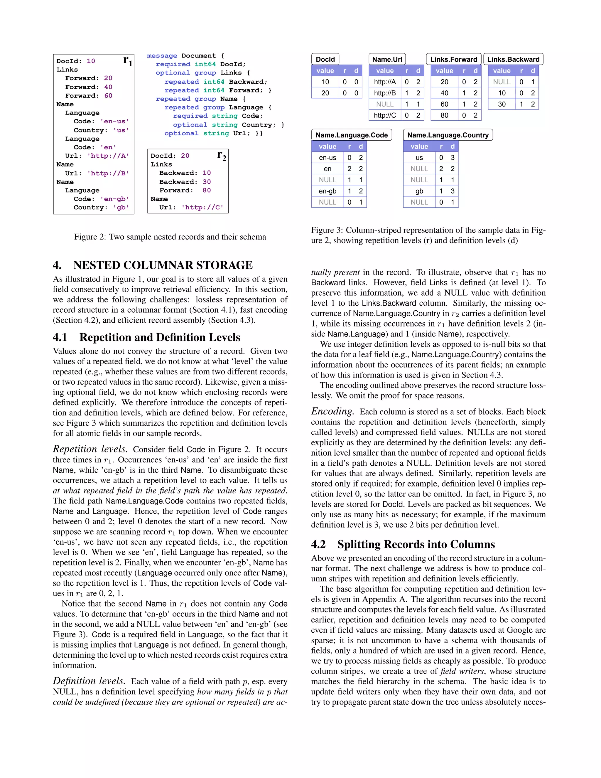
To illustrate, consider Figure 2. It depicts a schema that defines a
record type Document, representing a web document. The schema
definition uses the concrete syntax from [21]. A Document has a re-
quired integer DocId and optional Links, containing a list of Forward
and Backward entries holding DocIds of other web pages. A docu-
ment can have multiple Names, which are different URLs by which
the document can be referenced. A Name contains a sequence of
Code and (optional) Country pairs. Figure 2 also shows two sample
records, r1 and r2, conforming to the schema. The record structure
is outlined using indentation. We will use these sample records to
explain the algorithms in the next sections. The fields defined in the
schema form a tree hierarchy. The full path of a nested field is de-
noted using the usual dotted notation, e.g., Name.Language.Code.
The nested data model backs a platform-neutral, extensible
mechanism for serializing structured data at Google. Code gen-
eration tools produce bindings for programming languages such
as C++ or Java. Cross-language interoperability is achieved using
a standard binary on-the-wire representation of records, in which
field values are laid out sequentially as they occur in the record.
This way, a MR program written in Java can consume records from
a data source exposed via a C++ library. Thus, if records are stored
in a columnar representation, assembling them fast is important for
interoperation with MR and other data processing tools.

3. DocId: 10
Links
Forward: 20
Forward: 40
Forward: 60
Name
Language
Code: 'en-us'
Country: 'us'
Language
Code: 'en'
Url: 'http://A'
Name
Url: 'http://B'
Name
Language
Code: 'en-gb'
Country: 'gb'
r1
message Document {
required int64 DocId;
optional group Links {
repeated int64 Backward;
repeated int64 Forward; }
repeated group Name {
repeated group Language {
required string Code;
optional string Country; }
optional string Url; }}
DocId: 20
Links
Backward: 10
Backward: 30
Forward: 80
Name
Url: 'http://C'
r2
Figure 2: Two sample nested records and their schema
4. NESTED COLUMNAR STORAGE
As illustrated in Figure 1, our goal is to store all values of a given
field consecutively to improve retrieval efficiency. In this section,
we address the following challenges: lossless representation of
record structure in a columnar format (Section 4.1), fast encoding
(Section 4.2), and efficient record assembly (Section 4.3).
4.1 Repetition and Definition Levels
Values alone do not convey the structure of a record. Given two
values of a repeated field, we do not know at what ‘level’ the value
repeated (e.g., whether these values are from two different records,
or two repeated values in the same record). Likewise, given a miss-
ing optional field, we do not know which enclosing records were
defined explicitly. We therefore introduce the concepts of repeti-
tion and definition levels, which are defined below. For reference,
see Figure 3 which summarizes the repetition and definition levels
for all atomic fields in our sample records.
Repetition levels. Consider field Code in Figure 2. It occurs
three times in r1. Occurrences ‘en-us’ and ‘en’ are inside the first
Name, while ’en-gb’ is in the third Name. To disambiguate these
occurrences, we attach a repetition level to each value. It tells us
at what repeated field in the field’s path the value has repeated.
The field path Name.Language.Code contains two repeated fields,
Name and Language. Hence, the repetition level of Code ranges
between 0 and 2; level 0 denotes the start of a new record. Now
suppose we are scanning record r1 top down. When we encounter
‘en-us’, we have not seen any repeated fields, i.e., the repetition
level is 0. When we see ‘en’, field Language has repeated, so the
repetition level is 2. Finally, when we encounter ‘en-gb’, Name has
repeated most recently (Language occurred only once after Name),
so the repetition level is 1. Thus, the repetition levels of Code val-
ues in r1 are 0, 2, 1.
Notice that the second Name in r1 does not contain any Code
values. To determine that ‘en-gb’ occurs in the third Name and not
in the second, we add a NULL value between ‘en’ and ‘en-gb’ (see
Figure 3). Code is a required field in Language, so the fact that it
is missing implies that Language is not defined. In general though,
determining the level up to which nested records exist requires extra
information.
Definition levels. Each value of a field with path p, esp. every
NULL, has a definition level specifying how many fields in p that
could be undefined (because they are optional or repeated) are ac-
value r d
10 0 0
20 0 0
DocId
value r d
http://A 0 2
http://B 1 2
NULL 1 1
http://C 0 2
Name.Url
value r d
en-us 0 2
en 2 2
NULL 1 1
en-gb 1 2
NULL 0 1
Name.Language.Code Name.Language.Country
Links.BackwardLinks.Forward
value r d
us 0 3
NULL 2 2
NULL 1 1
gb 1 3
NULL 0 1
value r d
20 0 2
40 1 2
60 1 2
80 0 2
value r d
NULL 0 1
10 0 2
30 1 2
Figure 3: Column-striped representation of the sample data in Fig-
ure 2, showing repetition levels (r) and definition levels (d)
tually present in the record. To illustrate, observe that r1 has no
Backward links. However, field Links is defined (at level 1). To
preserve this information, we add a NULL value with definition
level 1 to the Links.Backward column. Similarly, the missing oc-
currence of Name.Language.Country in r2 carries a definition level
1, while its missing occurrences in r1 have definition levels 2 (in-
side Name.Language) and 1 (inside Name), respectively.
We use integer definition levels as opposed to is-null bits so that
the data for a leaf field (e.g., Name.Language.Country) contains the
information about the occurrences of its parent fields; an example
of how this information is used is given in Section 4.3.
The encoding outlined above preserves the record structure loss-
lessly. We omit the proof for space reasons.
Encoding. Each column is stored as a set of blocks. Each block
contains the repetition and definition levels (henceforth, simply
called levels) and compressed field values. NULLs are not stored
explicitly as they are determined by the definition levels: any defi-
nition level smaller than the number of repeated and optional fields
in a field’s path denotes a NULL. Definition levels are not stored
for values that are always defined. Similarly, repetition levels are
stored only if required; for example, definition level 0 implies rep-
etition level 0, so the latter can be omitted. In fact, in Figure 3, no
levels are stored for DocId. Levels are packed as bit sequences. We
only use as many bits as necessary; for example, if the maximum
definition level is 3, we use 2 bits per definition level.
4.2 Splitting Records into Columns
Above we presented an encoding of the record structure in a colum-
nar format. The next challenge we address is how to produce col-
umn stripes with repetition and definition levels efficiently.
The base algorithm for computing repetition and definition lev-
els is given in Appendix A. The algorithm recurses into the record
structure and computes the levels for each field value. As illustrated
earlier, repetition and definition levels may need to be computed
even if field values are missing. Many datasets used at Google are
sparse; it is not uncommon to have a schema with thousands of
fields, only a hundred of which are used in a given record. Hence,
we try to process missing fields as cheaply as possible. To produce
column stripes, we create a tree of field writers, whose structure
matches the field hierarchy in the schema. The basic idea is to
update field writers only when they have their own data, and not
try to propagate parent state down the tree unless absolutely neces-

4. Name.Language.CountryName.Language.Code
Links.Backward Links.Forward
Name.Url
DocId
1
0
1
0
0,1,2
2
0,11
0
0
Figure 4: Complete record assembly automaton. Edges are labeled
with repetition levels.
DocId
Name.Language.Country1,2
0
0
DocId: 10
Name
Language
Country: 'us'
Language
Name
Language
Country: 'gb'
DocId: 20
Name
s1
s2
Figure 5: Automaton for assembling records from two fields, and
the records it produces
sary. To do that, child writers inherit the levels from their parents.
A child writer synchronizes to its parent’s levels whenever a new
value is added.
4.3 Record Assembly
Assembling records from columnar data efficiently is critical for
record-oriented data processing tools (e.g., MR). Given a subset of
fields, our goal is to reconstruct the original records as if they con-
tained just the selected fields, with all other fields stripped away.
The key idea is this: we create a finite state machine (FSM) that
reads the field values and levels for each field, and appends the val-
ues sequentially to the output records. An FSM state corresponds
to a field reader for each selected field. State transitions are labeled
with repetition levels. Once a reader fetches a value, we look at the
next repetition level to decide what next reader to use. The FSM is
traversed from the start to end state once for each record.
Figure 4 shows an FSM that reconstructs the complete records
in our running example. The start state is DocId. Once a DocId
value is read, the FSM transitions to Links.Backward. After all
repeated Backward values have been drained, the FSM jumps to
Links.Forward, etc. The details of the record assembly algorithm
are in Appendix B.
To sketch how FSM transitions are constructed, let l be the next
repetition level returned by the current field reader for field f. Start-
ing at f in the schema tree, we find its ancestor that repeats at level l
and select the first leaf field n inside that ancestor. This gives us an
FSM transition (f, l) → n. For example, let l = 1 be the next repe-
tition level read by f = Name.Language.Country. Its ancestor with
repetition level 1 is Name, whose first leaf field is n = Name.Url.
The details of the FSM construction algorithm are in Appendix C.
If only a subset of fields need to be retrieved, we construct a
simpler FSM that is cheaper to execute. Figure 5 depicts an FSM
for reading the fields DocId and Name.Language.Country. The
figure shows the output records s1 and s2 produced by the au-
tomaton. Notice that our encoding and the assembly algorithm
Id: 10
Name
Cnt: 2
Language
Str: 'http://A,en-us'
Str: 'http://A,en'
Name
Cnt: 0
t1
SELECT DocId AS Id,
COUNT(Name.Language.Code) WITHIN Name AS Cnt,
Name.Url + ',' + Name.Language.Code AS Str
FROM t
WHERE REGEXP(Name.Url, '^http') AND DocId < 20;
message QueryResult {
required int64 Id;
repeated group Name {
optional uint64 Cnt;
repeated group Language {
optional string Str; }}}
Figure 6: Sample query, its result, and output schema
preserve the enclosing structure of the field Country. This is im-
portant for applications that need to access, e.g., the Country ap-
pearing in the first Language of the second Name. In XPath,
this would correspond to the ability to evaluate expressions like
/Name[2]/Language[1]/Country.
5. QUERY LANGUAGE
Dremel’s query language is based on SQL and is designed to be
efficiently implementable on columnar nested storage. Defining
the language formally is out of scope of this paper; instead, we il-
lustrate its flavor. Each SQL statement (and algebraic operators it
translates to) takes as input one or multiple nested tables and their
schemas and produces a nested table and its output schema. Fig-
ure 6 depicts a sample query that performs projection, selection,
and within-record aggregation. The query is evaluated over the ta-
ble t = {r1, r2} from Figure 2. The fields are referenced using
path expressions. The query produces a nested result although no
record constructors are present in the query.
To explain what the query does, consider the selection operation
(the WHERE clause). Think of a nested record as a labeled tree,
where each label corresponds to a field name. The selection op-
erator prunes away the branches of the tree that do not satisfy the
specified conditions. Thus, only those nested records are retained
where Name.Url is defined and starts with http. Next, consider pro-
jection. Each scalar expression in the SELECT clause emits a value
at the same level of nesting as the most-repeated input field used in
that expression. So, the string concatenation expression emits Str
values at the level of Name.Language.Code in the input schema.
The COUNT expression illustrates within-record aggregation. The
aggregation is done WITHIN each Name subrecord, and emits the
number of occurrences of Name.Language.Code for each Name as
a non-negative 64-bit integer (uint64).
The language supports nested subqueries, inter and intra-record
aggregation, top-k, joins, user-defined functions, etc; some of these
features are exemplified in the experimental section.
6. QUERY EXECUTION
We discuss the core ideas in the context of a read-only system, for
simplicity. Many Dremel queries are one-pass aggregations; there-
fore, we focus on explaining those and use them for experiments
in the next section. We defer the discussion of joins, indexing, up-
dates, etc. to future work.
Tree architecture. Dremel uses a multi-level serving tree to
execute queries (see Figure 7). A root server receives incoming
queries, reads metadata from the tables, and routes the queries to
the next level in the serving tree. The leaf servers communicate

5. query execution tree
. . .
. . .
. . .
storage layer (e.g., GFS)
. . .
. . .
. . .leaf servers
(with local
storage)
intermediate
servers
root server
client
Figure 7: System architecture and execution inside a server node
with the storage layer or access the data on local disk. Consider a
simple aggregation query below:
SELECT A, COUNT(B) FROM T GROUP BY A
When the root server receives the above query, it determines all
tablets, i.e., horizontal partitions of the table, that comprise T and
rewrites the query as follows:
SELECT A, SUM(c) FROM (R1
1 UNION ALL ... R1
n) GROUP BY A
Tables R1
1, . . . , R1
n are the results of queries sent to the nodes
1, . . . , n at level 1 of the serving tree:
R1
i = SELECT A, COUNT(B) AS c FROM T1
i GROUP BY A
T1
i is a disjoint partition of tablets in T processed by server i
at level 1. Each serving level performs a similar rewriting. Ulti-
mately, the queries reach the leaves, which scan the tablets in T in
parallel. On the way up, intermediate servers perform a parallel ag-
gregation of partial results. The execution model presented above
is well-suited for aggregation queries returning small and medium-
sized results, which are a very common class of interactive queries.
Large aggregations and other classes of queries may need to rely
on execution mechanisms known from parallel DBMSs and MR.
Query dispatcher. Dremel is a multi-user system, i.e., usually
several queries are executed simultaneously. A query dispatcher
schedules queries based on their priorities and balances the load. Its
other important role is to provide fault tolerance when one server
becomes much slower than others or a tablet replica becomes un-
reachable.
The amount of data processed in each query is often larger than
the number of processing units available for execution, which we
call slots. A slot corresponds to an execution thread on a leaf server.
For example, a system of 3,000 leaf servers each using 8 threads
has 24,000 slots. So, a table spanning 100,000 tablets can be pro-
cessed by assigning about 5 tablets to each slot. During query ex-
ecution, the query dispatcher computes a histogram of tablet pro-
cessing times. If a tablet takes a disproportionately long time to
process, it reschedules it on another server. Some tablets may need
to be redispatched multiple times.
The leaf servers read stripes of nested data in columnar represen-
tation. The blocks in each stripe are prefetched asynchronously;
the read-ahead cache typically achieves hit rates of 95%. Tablets
are usually three-way replicated. When a leaf server cannot access
one tablet replica, it falls over to another replica.
The query dispatcher honors a parameter that specifies the min-
imum percentage of tablets that must be scanned before returning
a result. As we demonstrate shortly, setting such parameter to a
lower value (e.g., 98% instead of 100%) can often speed up execu-
Table
name
Number of
records
Size (unrepl.,
compressed)
Number
of fields
Data
center
Repl.
factor
T1 85 billion 87 TB 270 A 3×
T2 24 billion 13 TB 530 A 3×
T3 4 billion 70 TB 1200 A 3×
T4 1+ trillion 105 TB 50 B 3×
T5 1+ trillion 20 TB 30 B 2×
Figure 8: Datasets used in the experimental study
tion significantly, especially when using smaller replication factors.
Each server has an internal execution tree, as depicted on the
right-hand side of Figure 7. The internal tree corresponds to a phys-
ical query execution plan, including evaluation of scalar expres-
sions. Optimized, type-specific code is generated for most scalar
functions. An execution plan for project-select-aggregate queries
consists of a set of iterators that scan input columns in lockstep and
emit results of aggregates and scalar functions annotated with the
correct repetition and definition levels, bypassing record assembly
entirely during query execution. For details, see Appendix D.
Some Dremel queries, such as top-k and count-distinct, return
approximate results using known one-pass algorithms (e.g., [4]).
7. EXPERIMENTS
In this section we evaluate Dremel’s performance on several
datasets used at Google, and examine the effectiveness of colum-
nar storage for nested data. The properties of the datasets used
in our study are summarized in Figure 8. In uncompressed, non-
replicated form the datasets occupy about a petabyte of space. All
tables are three-way replicated, except one two-way replicated ta-
ble, and contain from 100K to 800K tablets of varying sizes. We
start by examining the basic data access characteristics on a single
machine, then show how columnar storage benefits MR execution,
and finally focus on Dremel’s performance. The experiments were
conducted on system instances running in two data centers next to
many other applications, during regular business operation. Un-
less specified otherwise, execution times were averaged across five
runs. Table and field names used below are anonymized.
Local disk. In the first experiment, we examine performance
tradeoffs of columnar vs. record-oriented storage, scanning a 1GB
fragment of table T1 containing about 300K rows (see Figure 9).
The data is stored on a local disk and takes about 375MB in com-
pressed columnar representation. The record-oriented format uses
heavier compression yet yields about the same size on disk. The
experiment was done on a dual-core Intel machine with a disk pro-
viding 70MB/s read bandwidth. All reported times are cold; OS
cache was flushed prior to each scan.
The figure shows five graphs, illustrating the time it takes to read
and uncompress the data, and assemble and parse the records, for a
subset of the fields. Graphs (a)-(c) outline the results for columnar
storage. Each data point in these graphs was obtained by averaging
the measurements over 30 runs, in each of which a set of columns of
a given cardinality was chosen at random. Graph (a) shows read-
ing and decompression time. Graph (b) adds the time needed to
assemble nested records from columns. Graph (c) shows how long
it takes to parse the records into strongly typed C++ data structures.
Graphs (d)-(e) depict the time for accessing the data on record-
oriented storage. Graph (d) shows reading and decompression time.
A bulk of the time is spent in decompression; in fact, the com-
pressed data can be read from the disk in about half the time. As

6. !"
#"
$"
%"
&"
'!"
'#"
'$"
'%"
'&"
#!"
'" #" (" $" )" %" *" &" +" '!"
columns
records
objects
fromrecordsfromcolumns
(a) read +
decompress
(b) assemble
records
(c) parse as
objects
(d) read +
decompress
(e) parse as
objects
time (sec)
number of fields
Figure 9: Performance breakdown when reading from a local disk
(300K-record fragment of Table T1)
Graph (e) indicates, parsing adds another 50% on top of reading
and decompression time. These costs are paid for all fields, includ-
ing the ones that are not needed.
The main takeaways of this experiment are the following: when
few columns are read, the gains of columnar representation are of
about an order of magnitude. Retrieval time for columnar nested
data grows linearly with the number of fields. Record assembly and
parsing are expensive, each potentially doubling the execution time.
We observed similar trends on other datasets. A natural question
to ask is where the top and bottom graphs cross, i.e., record-wise
storage starts outperforming columnar storage. In our experience,
the crossover point often lies at dozens of fields but it varies across
datasets and depends on whether or not record assembly is required.
MR and Dremel. Next we illustrate a MR and Dremel exe-
cution on columnar vs. record-oriented data. We consider a case
where a single field is accessed, i.e., the performance gains are
most pronounced. Execution times for multiple columns can be
extrapolated using the results of Figure 9. In this experiment, we
count the average number of terms in a field txtField of table T1.
MR execution is done using the following Sawzall [20] program:
numRecs: table sum of int;
numWords: table sum of int;
emit numRecs <- 1;
emit numWords <- CountWords(input.txtField);
The number of records is stored in the variable numRecs. For
each record, numWords is incremented by the number of terms
in input.txtField returned by the CountWords function. After the
program runs, the average term frequency can be computed as
numWords/numRecs. In SQL, this computation is expressed as:
Q1: SELECT SUM(CountWords(txtField)) / COUNT(*) FROM T1
Figure 10 shows the execution times of two MR jobs and Dremel
on a logarithmic scale. Both MR jobs are run on 3000 work-
ers. Similarly, a 3000-node Dremel instance is used to execute
Query Q1. Dremel and MR-on-columns read about 0.5TB of com-
pressed columnar data vs. 87TB read by MR-on-records. As the
figure illustrates, MR gains an order of magnitude in efficiency by
switching from record-oriented to columnar storage (from hours to
minutes). Another order of magnitude is achieved by using Dremel
(going from minutes to seconds).
Serving tree topology. In the next experiment, we show the
impact of the serving tree depth on query execution times. We
consider two GROUP BY queries on Table T2, each executed using
!"
!#"
!##"
!###"
!####"
$%&'()*'+," $%&)*-./0," 1'(/(-"
execution time (sec)
Figure 10: MR and Dremel execution on columnar vs. record-
oriented storage (3000 nodes, 85 billion records)
!"
#!"
$!"
%!"
&!"
'!"
(!"
)$" )%"
$"*+,+*-"
%"*+,+*-"
&"*+,+*-"
execution time (sec)
Figure 11: Execution time as a function of serving tree levels for
two aggregation queries on T2
a single scan over the data. Table T2 contains 24 billion nested
records. Each record has a repeated field item containing a numeric
amount. The field item.amount repeats about 40 billion times in the
dataset. The first query sums up the item amount by country:
Q2: SELECT country, SUM(item.amount) FROM T2
GROUP BY country
It returns a few hundred records and reads roughly 60GB of com-
pressed data from disk. The second query performs a GROUP BY
on a text field domain with a selection condition. It reads about
180GB and produces around 1.1 million distinct domains:
Q3: SELECT domain, SUM(item.amount) FROM T2
WHERE domain CONTAINS ’.net’
GROUP BY domain
Figure 11 shows the execution times for each query as a function
of the server topology. In each topology, the number of leaf servers
is kept constant at 2900 so that we can assume the same cumulative
scan speed. In the 2-level topology (1:2900), a single root server
communicates directly with the leaf servers. For 3 levels, we use
a 1:100:2900 setup, i.e., an extra level of 100 intermediate servers.
The 4-level topology is 1:10:100:2900.
Query Q2 runs in 3 seconds when 3 levels are used in the serv-
ing tree and does not benefit much from an extra level. In con-
trast, the execution time of Q3 is halved due to increased paral-
lelism. At 2 levels, Q3 is off the chart, as the root server needs
to aggregate near-sequentially the results received from thousands
of nodes. This experiment illustrates how aggregations returning
many groups benefit from multi-level serving trees.
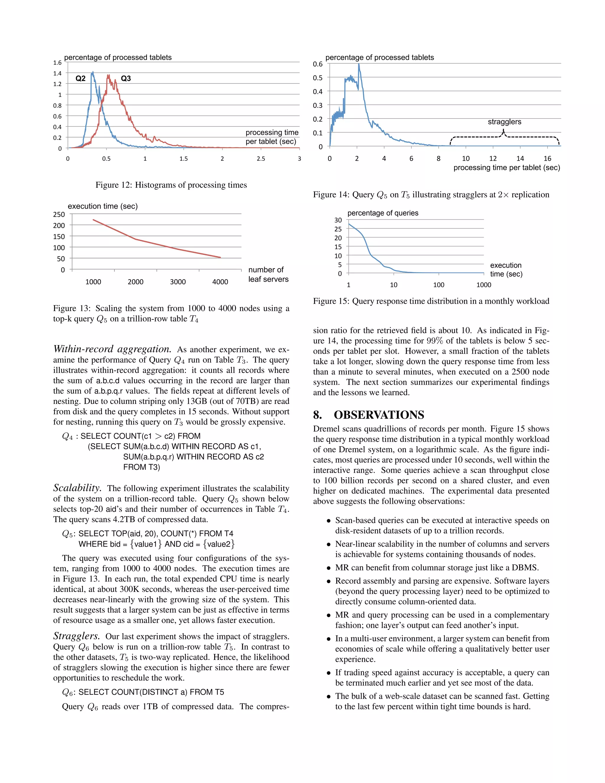
Per-tablet histograms. To drill deeper into what happens dur-
ing query execution consider Figure 12. The figure shows how fast
tablets get processed by the leaf servers for a specific run of Q2 and
Q3. The time is measured starting at the point when a tablet got
scheduled for execution in an available slot, i.e., excludes the time
spent waiting in the job queue. This measurement methodology
factors out the effects of other queries that are executing simulta-
neously. The area under each histogram corresponds to 100%. As
the figure indicates, 99% of Q2 (or Q3) tablets are processed under
one second (or two seconds).

7. !"
!#$"
!#%"
!#&"
!#'"
("
(#$"
(#%"
(#&"
!" !#)" (" (#)" $" $#)" *"
percentage of processed tablets
processing time
per tablet (sec)
Q3Q2
Figure 12: Histograms of processing times
!"
#!"
$!!"
$#!"
%!!"
%#!"
$!!!" %!!!" &!!!" '!!!"
execution time (sec)
number of
leaf servers
Figure 13: Scaling the system from 1000 to 4000 nodes using a
top-k query Q5 on a trillion-row table T4
Within-record aggregation. As another experiment, we ex-
amine the performance of Query Q4 run on Table T3. The query
illustrates within-record aggregation: it counts all records where
the sum of a.b.c.d values occurring in the record are larger than
the sum of a.b.p.q.r values. The fields repeat at different levels of
nesting. Due to column striping only 13GB (out of 70TB) are read
from disk and the query completes in 15 seconds. Without support
for nesting, running this query on T3 would be grossly expensive.
Q4 : SELECT COUNT(c1 > c2) FROM
(SELECT SUM(a.b.c.d) WITHIN RECORD AS c1,
SUM(a.b.p.q.r) WITHIN RECORD AS c2
FROM T3)
Scalability. The following experiment illustrates the scalability
of the system on a trillion-record table. Query Q5 shown below
selects top-20 aid’s and their number of occurrences in Table T4.
The query scans 4.2TB of compressed data.
Q5: SELECT TOP(aid, 20), COUNT(*) FROM T4
WHERE bid = {value1} AND cid = {value2}
The query was executed using four configurations of the sys-
tem, ranging from 1000 to 4000 nodes. The execution times are
in Figure 13. In each run, the total expended CPU time is nearly
identical, at about 300K seconds, whereas the user-perceived time
decreases near-linearly with the growing size of the system. This
result suggests that a larger system can be just as effective in terms
of resource usage as a smaller one, yet allows faster execution.
Stragglers. Our last experiment shows the impact of stragglers.
Query Q6 below is run on a trillion-row table T5. In contrast to
the other datasets, T5 is two-way replicated. Hence, the likelihood
of stragglers slowing the execution is higher since there are fewer
opportunities to reschedule the work.
Q6: SELECT COUNT(DISTINCT a) FROM T5
Query Q6 reads over 1TB of compressed data. The compres-
!"
!#$"
!#%"
!#&"
!#'"
!#("
!#)"
!" %" '" )" *" $!" $%" $'" $)"
percentage of processed tablets
processing time per tablet (sec)
stragglers
Figure 14: Query Q5 on T5 illustrating stragglers at 2× replication
!"
#"
$!"
$#"
%!"
%#"
&!"
$" $!" $!!" $!!!"
execution
time (sec)
percentage of queries
Figure 15: Query response time distribution in a monthly workload
sion ratio for the retrieved field is about 10. As indicated in Fig-
ure 14, the processing time for 99% of the tablets is below 5 sec-
onds per tablet per slot. However, a small fraction of the tablets
take a lot longer, slowing down the query response time from less
than a minute to several minutes, when executed on a 2500 node
system. The next section summarizes our experimental findings
and the lessons we learned.
8. OBSERVATIONS
Dremel scans quadrillions of records per month. Figure 15 shows
the query response time distribution in a typical monthly workload
of one Dremel system, on a logarithmic scale. As the figure indi-
cates, most queries are processed under 10 seconds, well within the
interactive range. Some queries achieve a scan throughput close
to 100 billion records per second on a shared cluster, and even
higher on dedicated machines. The experimental data presented
above suggests the following observations:
• Scan-based queries can be executed at interactive speeds on
disk-resident datasets of up to a trillion records.
• Near-linear scalability in the number of columns and servers
is achievable for systems containing thousands of nodes.
• MR can benefit from columnar storage just like a DBMS.
• Record assembly and parsing are expensive. Software layers
(beyond the query processing layer) need to be optimized to
directly consume column-oriented data.
• MR and query processing can be used in a complementary
fashion; one layer’s output can feed another’s input.
• In a multi-user environment, a larger system can benefit from
economies of scale while offering a qualitatively better user
experience.
• If trading speed against accuracy is acceptable, a query can
be terminated much earlier and yet see most of the data.
• The bulk of a web-scale dataset can be scanned fast. Getting
to the last few percent within tight time bounds is hard.

8. Dremel’s codebase is dense; it comprises less than 100K lines of
C++, Java, and Python code.
9. RELATED WORK
The MapReduce (MR) [12] framework was designed to address the
challenges of large-scale computing in the context of long-running
batch jobs. Like MR, Dremel provides fault tolerant execution, a
flexible data model, and in situ data processing capabilities. The
success of MR led to a wide range of third-party implementations
(notably open-source Hadoop [15]), and a number of hybrid sys-
tems that combine parallel DBMSs with MR, offered by vendors
like Aster, Cloudera, Greenplum, and Vertica. HadoopDB [3] is
a research system in this hybrid category. Recent articles [13, 22]
contrast MR and parallel DBMSs. Our work emphasizes the com-
plementary nature of both paradigms.
Dremel is designed to operate at scale. Although it is conceivable
that parallel DBMSs can be made to scale to thousands of nodes,
we are not aware of any published work or industry reports that at-
tempted that. Neither are we familiar with prior literature studying
MR on columnar storage.
Our columnar representation of nested data builds on ideas that
date back several decades: separation of structure from content
and transposed representation. A recent review of work on col-
umn stores, incl. compression and query processing, can be found
in [1]. Many commercial DBMSs support storage of nested data
using XML (e.g., [19]). XML storage schemes attempt to separate
the structure from the content but face more challenges due to the
flexibility of the XML data model. One system that uses columnar
XML representation is XMill [17]. XMill is a compression tool.
It stores the structure for all fields combined and is not geared for
selective retrieval of columns.
The data model used in Dremel is a variation of the com-
plex value models and nested relational models discussed in [2].
Dremel’s query language builds on the ideas from [9], which intro-
duced a language that avoids restructuring when accessing nested
data. In contrast, restructuring is usually required in XQuery and
object-oriented query languages, e.g., using nested for-loops and
constructors. We are not aware of practical implementations of [9].
A recent SQL-like language operating on nested data is Pig [18].
Other systems for parallel data processing include Scope [6] and
DryadLINQ [23], and are discussed in more detail in [7].
10. CONCLUSIONS
We presented Dremel, a distributed system for interactive analy-
sis of large datasets. Dremel is a custom, scalable data manage-
ment solution built from simpler components. It complements the
MR paradigm. We discussed its performance on trillion-record,
multi-terabyte datasets of real data. We outlined the key aspects
of Dremel, including its storage format, query language, and exe-
cution. In the future, we plan to cover in more depth such areas as
formal algebraic specification, joins, extensibility mechanisms, etc.
11. ACKNOWLEDGEMENTS
Dremel has benefited greatly from the input of many engineers and
interns at Google, in particular Craig Chambers, Ori Gershoni, Ra-
jeev Byrisetti, Leon Wong, Erik Hendriks, Erika Rice Scherpelz,
Charlie Garrett, Idan Avraham, Rajesh Rao, Andy Kreling, Li Yin,
Madhusudan Hosaagrahara, Dan Belov, Brian Bershad, Lawrence
You, Rongrong Zhong, Meelap Shah, and Nathan Bales.
12. REFERENCES
[1] D. J. Abadi, P. A. Boncz, and S. Harizopoulos.
Column-Oriented Database Systems. VLDB, 2(2), 2009.
[2] S. Abiteboul, R. Hull, and V. Vianu. Foundations of
Databases. Addison Wesley, 1995.
[3] A. Abouzeid, K. Bajda-Pawlikowski, D. J. Abadi, A. Rasin,
and A. Silberschatz. HadoopDB: An Architectural Hybrid of
MapReduce and DBMS Technologies for Analytical
Workloads. VLDB, 2(1), 2009.
[4] Z. Bar-Yossef, T. S. Jayram, R. Kumar, D. Sivakumar, and
L. Trevisan. Counting Distinct Elements in a Data Stream. In
RANDOM, pages 1–10, 2002.
[5] L. A. Barroso and U. H¨olzle. The Datacenter as a Computer:
An Introduction to the Design of Warehouse-Scale Machines.
Morgan & Claypool Publishers, 2009.
[6] R. Chaiken, B. Jenkins, P.-A. Larson, B. Ramsey, D. Shakib,
S. Weaver, and J. Zhou. SCOPE: Easy and Efficient Parallel
Processing of Massive Data Sets. VLDB, 1(2), 2008.
[7] C. Chambers, A. Raniwala, F. Perry, S. Adams, R. Henry,
R. Bradshaw, and N. Weizenbaum. FlumeJava: Easy,
Efficient Data-Parallel Pipelines. In PLDI, 2010.
[8] F. Chang, J. Dean, S. Ghemawat, W. C. Hsieh, D. A.
Wallach, M. Burrows, T. Chandra, A. Fikes, and R. Gruber.
Bigtable: A Distributed Storage System for Structured Data.
In OSDI, 2006.
[9] L. S. Colby. A Recursive Algebra and Query Optimization
for Nested Relations. SIGMOD Rec., 18(2), 1989.
[10] G. Czajkowski. Sorting 1PB with MapReduce. Official
Google Blog, Nov. 2008. At http://googleblog.blogspot.com/
2008/11/sorting-1pb-with-mapreduce.html.
[11] J. Dean. Challenges in Building Large-Scale Information
Retrieval Systems: Invited Talk. In WSDM, 2009.
[12] J. Dean and S. Ghemawat. MapReduce: Simplified Data
Processing on Large Clusters. In OSDI, 2004.
[13] J. Dean and S. Ghemawat. MapReduce: a Flexible Data
Processing Tool. Commun. ACM, 53(1), 2010.
[14] S. Ghemawat, H. Gobioff, and S.-T. Leung. The Google File
System. In SOSP, 2003.
[15] Hadoop Apache Project. http://hadoop.apache.org.
[16] Hive. http://wiki.apache.org/hadoop/Hive, 2009.
[17] H. Liefke and D. Suciu. XMill: An Efficient Compressor for
XML Data. In SIGMOD, 2000.
[18] C. Olston, B. Reed, U. Srivastava, R. Kumar, and
A. Tomkins. Pig Latin: a Not-so-Foreign Language for Data
Processing. In SIGMOD, 2008.
[19] P. E. O’Neil, E. J. O’Neil, S. Pal, I. Cseri, G. Schaller, and
N. Westbury. ORDPATHs: Insert-Friendly XML Node
Labels. In SIGMOD, 2004.
[20] R. Pike, S. Dorward, R. Griesemer, and S. Quinlan.
Interpreting the Data: Parallel Analysis with Sawzall.
Scientific Programming, 13(4), 2005.
[21] Protocol Buffers: Developer Guide. Available at
http://code.google.com/apis/protocolbuffers/docs/overview.html.
[22] M. Stonebraker, D. Abadi, D. J. DeWitt, S. Madden,
E. Paulson, A. Pavlo, and A. Rasin. MapReduce and Parallel
DBMSs: Friends or Foes? Commun. ACM, 53(1), 2010.
[23] Y. Yu, M. Isard, D. Fetterly, M. Budiu, ´U. Erlingsson, P. K.
Gunda, and J. Currey. DryadLINQ: A System for
General-Purpose Distributed Data-Parallel Computing Using
a High-Level Language. In OSDI, 2008.

9. 1 procedure DissectRecord(RecordDecoder decoder,
2 FieldWriter writer, int repetitionLevel):
3 Add current repetitionLevel and definition level to writer
4 seenFields = {} // empty set of integers
5 while decoder has more field values
6 FieldWriter chWriter =
7 child of writer for field read by decoder
8 int chRepetitionLevel = repetitionLevel
9 if set seenFields contains field ID of chWriter
10 chRepetitionLevel = tree depth of chWriter
11 else
12 Add field ID of chWriter to seenFields
13 end if
14 if chWriter corresponds to an atomic field
15 Write value of current field read by decoder
16 using chWriter at chRepetitionLevel
17 else
18 DissectRecord(new RecordDecoder for nested record
19 read by decoder, chWriter, chRepetitionLevel)
20 end if
21 end while
22 end procedure
Figure 16: Algorithm for dissecting a record into columns
APPENDIX
A. COLUMN-STRIPING ALGORITHM
The algorithm for decomposing a record into columns is shown
in Figure 16. Procedure DissectRecord is passed an instance of a
RecordDecoder, which is used to traverse binary-encoded records.
FieldWriters form a tree hierarchy isomorphic to that of the input
schema. The root FieldWriter is passed to the algorithm for each
new record, with repetitionLevel set to 0. The primary job of the
DissectRecord procedure is to maintain the current repetitionLevel.
The current definitionLevel is uniquely determined by the tree posi-
tion of the current writer, as the sum of the number of optional and
repeated fields in the field’s path.
The while-loop of the algorithm (Line 5) iterates over all atomic
and record-valued fields contained in a given record. The set
seenFields tracks whether or not a field has been seen in the
record. It is used to determine what field has repeated most re-
cently. The child repetition level chRepetitionLevel is set to that
of the most recently repeated field or else defaults to its parent’s
level (Lines 9-13). The procedure is invoked recursively on nested
records (Line 18).
In Section 4.2 we sketched how FieldWriters accumulate levels
and propagate them lazily to lower-level writers. This is done as
follows: each non-leaf writer keeps a sequence of (repetition, def-
inition) levels. Each writer also has a ‘version’ number associated
with it. Simply stated, a writer version is incremented by one when-
ever a level is added. It is sufficient for children to remember the
last parent’s version they synced. If a child writer ever gets its own
(non-null) value, it synchronizes its state with the parent by fetch-
ing new levels, and only then adds the new data.
Because input data can have thousands of fields and millions
records, it is not feasible to store all levels in memory. Some levels
may be temporarily stored in a file on disk. For a lossless encoding
of empty (sub)records, non-atomic fields (such as Name.Language
in Figure 2) may need to have column stripes of their own, contain-
ing only levels but no non-NULL values.
B. RECORD ASSEMBLY ALGORITHM
In their on-the-wire representation, records are laid out as pairs of
1 Record AssembleRecord(FieldReaders[] readers):
2 record = create a new record
3 lastReader = select the root field reader in readers
4 reader = readers[0]
5 while reader has data
6 Fetch next value from reader
7 if current value is not NULL
8 MoveToLevel(tree level of reader, reader)
9 Append reader's value to record
10 else
11 MoveToLevel(full definition level of reader, reader)
12 end if
13 reader = reader that FSM transitions to
14 when reading next repetition level from reader
15 ReturnToLevel(tree level of reader)
16 end while
17 ReturnToLevel(0)
18 End all nested records
19 return record
20 end procedure
21
22 MoveToLevel(int newLevel, FieldReader nextReader):
23 End nested records up to the level of the lowest common ancestor
24 of lastReader and nextReader.
25 Start nested records from the level of the lowest common ancestor
26 up to newLevel.
27 Set lastReader to the one at newLevel.
28 end procedure
29
30 ReturnToLevel(int newLevel) {
31 End nested records up to newLevel.
32 Set lastReader to the one at newLevel.
33 end procedure
Figure 17: Algorithm for assembling a record from columns
a field identifier followed by a field value. Nested records can be
thought of as having an ‘opening tag’ and a ‘closing tag’, similar to
XML (actual binary encoding may differ, see [21] for details). In
the following, writing opening tags is referred to as ‘starting’ the
record, and writing closing tags is called ’ending’ it.
AssembleRecord procedure takes as input a set of FieldReaders
and (implicitly) the FSM with state transitions between the readers.
Variable reader holds the current FieldReader in the main routine
(Line 4). Variable lastReader holds the last reader whose value
we appended to the record and is available to all three procedures
shown in Figure 17. The main while-loop is at Line 5. We fetch
the next value from the current reader. If the value is not NULL,
which is determined by looking at its definition level, we synchro-
nize the record being assembled to the record structure of the cur-
rent reader in the method MoveToLevel, and append the field value
to the record. Otherwise, we merely adjust the record structure
without appending any value—which needs to be done if empty
records are present. On Line 12, we use a ‘full definition level’.
Recall that the definition level factors out required fields (only re-
peated and optional fields are counted). Full definition level takes
all fields into account.
Procedure MoveToLevel transitions the record from the state of
the lastReader to that of the nextReader (see Line 22). For exam-
ple, suppose the lastReader corresponds to Links.Backward in Fig-
ure 2 and nextReader is Name.Language.Code. The method ends
the nested record Links and starts new records Name and Language,
in that order. Procedure ReturnsToLevel (Line 30) is a counterpart
of MoveToLevel that only ends current records without starting any
new ones.

10. 1 procedure ConstructFSM(Field[] fields):
2 for each field in fields:
3 maxLevel = maximal repetition level of field
4 barrier = next field after field or final FSM state otherwise
5 barrierLevel = common repetition level of field and barrier
6 for each preField before field whose
7 repetition level is larger than barrierLevel:
8 backLevel = common repetition level of preField and field
9 Set transition (field, backLevel) -> preField
10 end for
11 for each level in [barrierLevel+1..maxLevel]
12 that lacks transition from field:
13 Copy transition's destination from that of level-1
14 end for
15 for each level in [0..barrierLevel]:
16 Set transition (field, level) -> barrier
17 end for
18 end for
19 end procedure
Figure 18: Algorithm to construct a record assembly automaton
C. FSM CONSTRUCTION ALGORITHM
Figure 18 shows an algorithm for constructing a finite-state ma-
chine that performs record assembly. The algorithm takes as input
the fields that should be populated in the records, in the order in
which they appear in the schema. The algorithm uses a concept of
a ‘common repetition level’ of two fields, which is the repetition
level of their lowest common ancestor. For example, the common
repetition level of Links.Backward and Links.Forward equals 1. The
second concept is that of a ‘barrier’, which is the next field in the
sequence after the current one. The intuition is that we try to pro-
cess each field one by one until the barrier is hit and requires a jump
to a previously seen field.
The algorithm consists of three steps. In Step 1 (Lines 6-10),
we go through the common repetition levels backwards. These are
guaranteed to be non-increasing. For each repetition level we en-
counter, we pick the left-most field in the sequence—that is the one
we need to transition to when that repetition level is returned by a
FieldReader. In Step 2, we fill the gaps (Lines 11-14). The gaps
arise because not all repetition levels are present in the common
repetition levels computed at Line 8. In Step 3 (Lines 15-17), we
set transitions for all levels that are equal to or below the barrier
level to jump to the barrier field. If a FieldReader produces such
a level, we need to continue constructing the nested record and do
not need to bounce off the barrier.
D. SELECT-PROJECT-AGGREGATE
EVALUATION ALGORITHM
Figure 19 shows the algorithm used for evaluating select-project-
aggregate queries in Dremel. The algorithm addresses a general
case when a query may reference repeated fields; a simpler opti-
mized version is used for flat-relational queries, i.e., those refer-
encing only required and optional fields. The algorithm has two
implicit inputs: a set of FieldReaders, one for each field appearing
in the query, and a set of scalar expressions, including aggregate
expressions, present in the query. The repetition level of a scalar
expression (used in Line 8) is determined as the maximum repeti-
tion level of the fields used in that expression.
In essence, the algorithm advances the readers in lockstep to the
next set of values, and, if the selection conditions are met, emits
the projected values. Selection and projection are controlled by
two variables, fetchLevel and selectLevel. During execution, only
1 procedure Scan():
2 fetchLevel = 0
3 selectLevel = 0
4 while stopping conditions are not met:
5 Fetch()
6 if WHERE clause evaluates to true:
7 for each expression in SELECT clause:
8 if (repetition level of expression) >= selectLevel:
9 Emit value of expression
10 end if
11 end for
12 selectLevel = fetchLevel
13 else
14 selectLevel = min(selectLevel, fetchLevel)
15 end if
16 end while
17 end procedure
18
19 procedure Fetch():
20 nextLevel = 0
21 for each reader in field reader set:
22 if (next repetition level of reader) >= fetchLevel:
23 Advance reader to the next value
24 endif
25 nextLevel = max(nextLevel, next repetition level of reader)
26 end for
27 fetchLevel = nextLevel
28 end procedure
Figure 19: Algorithm for evaluating select-project-aggregate
queries over columnar input, bypassing record assembly
readers whose next repetition level is no less than fetchLevel are
advanced (see Fetch method at Line 19). In a similar vein, only ex-
pressions whose current repetition level is no less than selectLevel
are emitted (Lines 7-10). The algorithm ensures that expressions
at a higher-level of nesting, i.e., those having a smaller repetition
level, get evaluated and emitted only once for each deeper nested
expression.