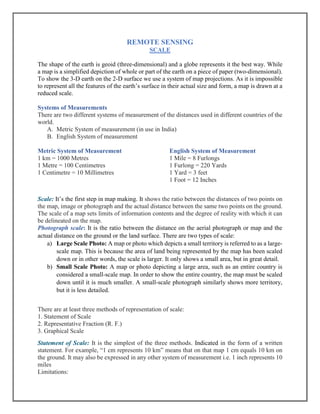
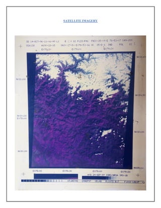
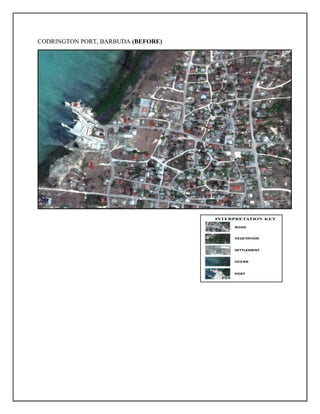
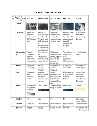
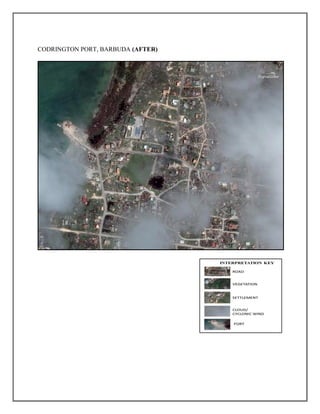
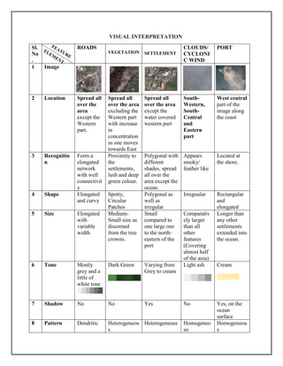
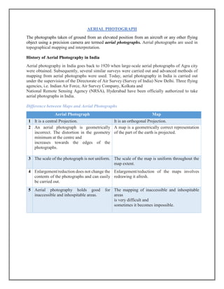
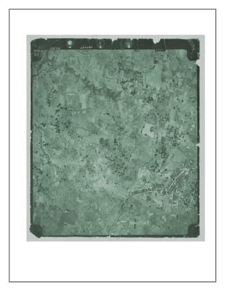
The document explains the principles of remote sensing and map-making, emphasizing the differences between three-dimensional geoid representation and two-dimensional maps. It covers measurement systems, scale types, and methods of representing scales, along with practical applications in visual interpretation of satellite imagery. Additionally, it highlights elements such as tone, texture, size, shape, shadow, and resolution that aid in analyzing satellite images for environmental monitoring and land use assessment.
![• The people who are familiar with one system may not understand the statement of scale in
another system of measurement.
• If the map is reduced or enlarged, the scale will become superfluous and a new scale is to
be worked out.
Graphical or Bar Scale: This scale shows map distances and the corresponding ground distances
using a line bar with primary and secondary divisions marked on it. Unlike the statement of the
scale method, the graphical scale stands valid even when the map is reduced or enlarged.
Representative Fraction (R. F.): The most versatile method representing the relationship between
the map distance and the corresponding ground distance in units of length. It is generally shown
in fraction because it shows how much the real world is reduced to fit on the map. For example, a
fraction of 1: 25,000 shows that one unit of length on the map represents 25,000 of the same units
on the ground. It may, however, be noted that while converting the fraction of units into Metric
or English systems, units in centimeter or inch are normally used by convention. This quality of
expressing scale in units in R. F. makes it a universally acceptable and usable method.
Relationship Between Photo Distance and Map Distance
Photo scale: Map scale = Photo distance: Map distance
Focal Length (f): Flying Height(H) = Photo distance (PD): Ground distance (GD)
Formulae
𝑷𝒉𝒐𝒕𝒐 𝑺𝒄𝒂𝒍𝒆 =
𝒇𝒐𝒄𝒂𝒍 𝒍𝒆𝒏𝒈𝒕𝒉
𝑯𝒆𝒊𝒈𝒉𝒕 𝒐𝒇 𝒕𝒉𝒆 𝒂𝒊𝒓𝒄𝒓𝒂𝒇𝒕
[𝑷. 𝑺. =
𝒇
𝑯
]
𝑷𝒉𝒐𝒕𝒐 𝑺𝒄𝒂𝒍𝒆
=
𝒇𝒐𝒄𝒂𝒍 𝒍𝒆𝒏𝒈𝒕𝒉
𝑯𝒆𝒊𝒈𝒉𝒕 𝒐𝒇 𝒕𝒉𝒆 𝒂𝒊𝒓𝒄𝒓𝒂𝒇𝒕 − 𝒉𝒆𝒊𝒈𝒉𝒕 𝒐𝒇 𝒕𝒆𝒓𝒓𝒂𝒊𝒏
[𝑷. 𝑺. =
𝒇
𝑯 − 𝒉
]
𝑷𝒉𝒐𝒕𝒐 𝑺𝒄𝒂𝒍𝒆 =
𝑷𝒉𝒐𝒕𝒐 𝑫𝒊𝒔𝒕𝒂𝒏𝒄𝒆
𝑮𝒓𝒐𝒖𝒏𝒅 𝑫𝒊𝒔𝒕𝒂𝒏𝒄𝒆
𝑴𝒂𝒑 𝑺𝒄𝒂𝒍𝒆 =
𝑴𝒂𝒑 𝑫𝒊𝒔𝒕𝒂𝒏𝒄𝒆
𝑮𝒓𝒐𝒖𝒏𝒅 𝑫𝒊𝒔𝒕𝒂𝒏𝒄𝒆
𝑮𝒓𝒐𝒖𝒏𝒅 𝑫𝒊𝒔𝒕𝒂𝒏𝒄𝒆 =
𝑷𝒉𝒐𝒕𝒐 𝑫𝒊𝒔𝒕𝒂𝒏𝒄𝒆
𝑷𝒉𝒐𝒕𝒐 𝑺𝒄𝒂𝒍𝒆](https://image.slidesharecdn.com/digitalimagelinearstretching-180329171023/85/Digital-image-linear-stretching-2-320.jpg)
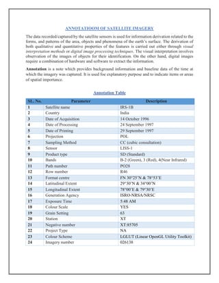
![SAMPLE QUESTION & ANSWERS
Question 1: If the focal length of the camera is 151.8mm and the aircraft is at 2000meters, with
the given terrain height of 500m. Find the photo scale of the aerial photograph.
Solution:
Given: Focal length = 151.8 mm.~ 0.1518 m. (∵ 1m=1000mm.)
Height of the aircraft =2000m
Terrain height =500m
To find: Photo scale
𝑃. 𝑆. =
𝑓
𝐻 − ℎ
=
0.1518
2000 − 500
=
0.1518
1500
=
1
9881.42
~
1
10,000
∴ P.S.= 1:10,000
Question 2. Find the scale of the aerial photograph, if focal length of the camera is 151.8mm and
height of the flying aircraft 600 ft.
Solution:
Given: Focal length = 151.8mm ~ 0.1518 m. (∵ 1m=1000mm.)
Height of the aircraft (H)= 600ft. ~ 181.81 (∵ 1m=3.3 ft.)
To Find: Photo scale (P.S.)
𝑃𝑆. =
𝑓𝑜𝑐𝑎𝑙 𝑙𝑒𝑛𝑔𝑡ℎ 𝑜𝑓 𝑡ℎ𝑒 𝑐𝑎𝑚𝑒𝑟𝑎
𝐹𝑙𝑦𝑖𝑛𝑔 ℎ𝑒𝑖𝑔ℎ𝑡 𝑜𝑓 𝑡ℎ𝑒 𝑎𝑖𝑟𝑐𝑟𝑎𝑓𝑡
[𝑃. 𝑆. =
𝑓
𝐻
]
=
0.1518
181.81
=
1
1197.7
∴ P.S.= 1:1200](https://image.slidesharecdn.com/digitalimagelinearstretching-180329171023/85/Digital-image-linear-stretching-3-320.jpg)
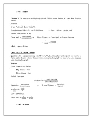

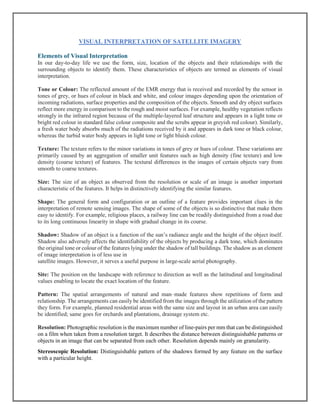


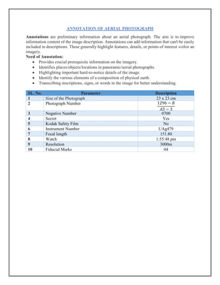
![Digital image are an array of digital numbers (DN) arranged in rows and columns, having the
property of an intensity value and their locations.
Formula:
Perform the linear stretch of the following 5X5 matrix of an 8-bit system
8-Bit system matrix (5X5)
31 38 45 49 89
73 75 85 89 100
95 95 93 89 110
110 111 93 89 150
110 111 93 89 150
DN (Maximum)=150
DN (Minimum)=31
DN (Input) Frequency
31 1
38 1
45 1
49 1
73 1
75 1
85 1
89 5
93 3
95 2
100 1
110 3
111 2
150 2
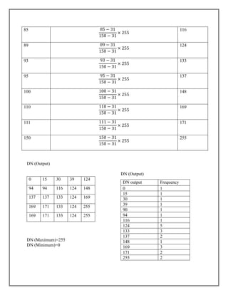
DN (Output) = [
𝐷𝑁 (𝐼𝑛𝑝𝑢𝑡) − 𝐷𝑁(𝑀𝑖𝑛𝑖𝑚𝑢𝑚)
𝐷𝑁 (𝑀𝑎𝑥𝑖𝑚𝑢𝑚) − 𝐷𝑁 (𝑀𝑖𝑛𝑖𝑚𝑢𝑚)
] × 255](https://image.slidesharecdn.com/digitalimagelinearstretching-180329171023/85/Digital-image-linear-stretching-23-320.jpg)
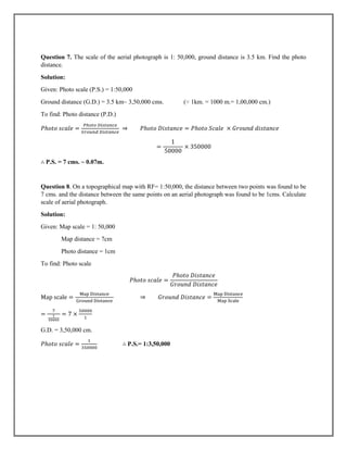
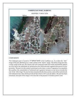
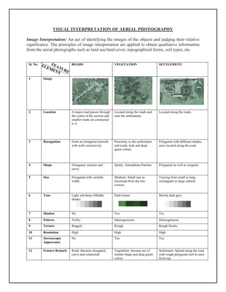
![DN input
Calculation
[𝐷𝑁 𝑜𝑢𝑡𝑝𝑢𝑡 =
𝐷𝑁 (𝑖𝑛𝑝𝑢𝑡) − 𝐷𝑁 (𝑚𝑖𝑛𝑖𝑚𝑢𝑚)
𝐷𝑁 (𝑚𝑎𝑥𝑖𝑚𝑢𝑚) − 𝐷𝑁 (𝑚𝑖𝑛𝑖𝑚𝑢𝑚)
× 255]
DN output
31 31 − 31
150 − 31
× 255
0
38 38 − 31
150 − 31
× 255
15
45 45 − 31
150 − 31
× 255
30
49 49 − 31
150 − 31
× 255
39
73 73 − 31
150 − 31
× 255
90
75 75 − 31
150 − 31
× 255
94
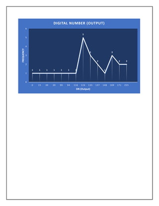
1 1 1 1 1 1 1
5
3
2
1
3
2 2
0
1
2
3
4
5
6
31 38 45 49 73 75 85 89 93 95 100 110 111 150 255
FREQUENCY
DN (Input)
DIGITAL NUMBER (INPUT)](https://image.slidesharecdn.com/digitalimagelinearstretching-180329171023/85/Digital-image-linear-stretching-24-320.jpg)