Power trasmission line energy saving through Machine Learning
1.
Feature Selection Techniquesfor Advanced Power System Fault
Analysis
By
Dr. Debani Prasad Mishra
ASST. PROFESSOR
(EE Department)
IIIT BHUBANESWAR
1
ONLINE FACULTY DEVELOPMENT PROGRAMME
(FDP) ON
Feature Engineering: The Backbone of Effective AI and
ML Solution Applications
(12th
– 23th
May 2025)
Organized by
Electronics & ICT Academy, NIT Warangal
In Association With
Department of CSE and EE,
International Institute of Information Technology (IIIT)
Bhubaneswar
Sponsored
by Ministry of Electronics and Information Technology
(MeitY), GoI
2.
TABLE OF CONTENT
Section-1 Introduction
1)General Overview
2) Importance of the work in the present scenario
3) Solution of the key problem
4) Objective of the proposed work
5) Literature Review
6) Entire protection scheme for fault classification and location
7) Detail structure for fault classification methods
8) Ground detection for fault classification methods
9) Performance criteria for fault classification and location method
10) Flow chat for fault location method
Section -II Combined signal processing and Machine learning based technique
1) Signal processing technique (DWT/ WPT / S Transform)
2) Feature selection technique (GA/ PSO/ FFS)
3) Artificial intelligence technique ( ANN/SVM /ELM)
2/93
3.
TABLE OF CONTENT
Section-III Fault classification and location of different configuration of the Transmission line
a) Fault classification and location of the Transmission line
1) System under study
2) Proposed Hybrid Technique
3) Results and Discussion
4) Comparison with other researcher
5) Conclusion
b) Fault classification and location of the Transmission line with TCSC
1) System under study
2) Proposed Hybrid Technique
3) Results and Discussion
4) Comparison with other researcher
5) Conclusion
3/93
4.
INTRODUCTION
Electric powersystems becoming complex and exposed to failure of their components.
Restore the supply, faulty element disconnected
Prolonged line outage and severe economic losses
Early repair to prevent recurrence and major damage
Restoration is done after the repair of the damage caused by the fault
Whole line has to be inspected to find the damaged place
Saving money and time for the inspection and repair
Better service due to faster restoration
Proper rectification, equipment replacement and re-evaluation of control strategies.
Continuous and uninterrupted power supply, fault classification and location is important
SECTION : I
4/93
5.
Transmission lines:765/ 400/220/132kV
EHT Customer:
400/220/132kV
Generating
Station
Generating
Step Up
Transformer
Substation
Step Down
Transformer
Sub-transmission
Customer 33kV
LT Customer
400V and 220V
SCHEMATIC DIAGRAM OF ELECTRICAL GRID
6.
INTRODUCTION
Classification andlocation of the fault is increased in application of a distribution line due to
the operation of deregulated environment and its tendency to compete in the power sector for
maximum availability of the power supply.
Protection engineers find challenges in certain applications like:-
Classification and Location of fault in a transmission and distribution line
Additional transients during fault which is not easily visible on inspection
Classification and location of fault in underground cable
repair requires large time and labour, cost is large, accuracy required is very high
To overcome the mentioned problems, following steps are taken:-
Necessary to develop an algorithm which can easily classify and locate the fault in a
transmission and distribution line. [1-3]
SECTION : I
6/93
7.
IMPORTANCE OF THEWORK IN THE PRESENT SCENARIO
Fault must be located properly, otherwise the whole line has to be inspected by the maintenance
and operation crew to find the exact location of the fault.
Proper classification and location identifies the part of the transmission line that has been
faulted
The patrolling vehicle of the transmission line operation and maintenance agency can reach the
spot at which the fault has occurred
Take up repair/correction activates without wasting any further time.
Tripping of lines in an important transmission corridor can lead to reduced levels of power
from one port of the country to the other (from a power surplus area to power starved area)
If important transmission line trip hunting of the system,
Collapse whole of the grid is also possible.
SECTION : I
7/93
8.
Outage timeis minimized/ Restoration of power supply becomes fast
Time and energy of the maintenance crew is reduced
Economic losses are reduced
Better Power Delivery
Reduces the computational complexity of learning and prediction
Unaffected by noise
Fault classification and location problem in series compensated transmission line is
eliminated.
Minimizes the fault classification and location errors
SOLUTION OF KEY PROBLEMS
SECTION -I
8/93
9.
OBJECTIVE OF THEPROPOSED WORK
The key objective of the is to develop a fast and correct fault classification and location method
for different configurations of transmission and distribution system.
To achieve the main goal, the following sub-objectives have to be met:
Effect of the shunt capacitance has to be eliminated
A Single cycle of post fault current and voltage signal has to be acquired for investigation
purpose.
Reduce the computation time and complexity of the the faulted data by using feature selection
technique.
Redundant features have to be removed and optimum features have to be chosen for the overall
feature set to enhance the prediction accuracy.
The simulation period required by the fault analyzer has to be reduced.
A robust fault analysis scheme has to be implemented which should be insensitive to parameter
changes.
To meet the above objective, an enhanced hybrid method is established to analysis the fault in
the transmission network.
SECTION : I
9/93
10.
LITERATURE REVIEW
Varioustechniques to estimate accurate fault location in a Transmission line
Impedance measurement based method
Single ended Impedance based method use line terminal voltage and current before and
during the fault
Test system (400 kV, 300 km)
Fault location error less than 1%.
The main drawback is that they have poor accuracy for high impedance fault.
SECTION : I
[Capar, A.; Arsoy, A. B. (2015) A performance oriented impedance based fault location
algorithm for series compensated transmission lines,” Electrical Power and Energy Systems 71
pp. 209–214 ]
10/93
For Transmission line
11.
LITERATURE REVIEW
Two-endedimpedance based technique is applied to localize the fault to eradicate the single
end impedance methods in the Transmission line.
The drawback of this technique is a high calculation burden due to measurement of current
and voltage signal at both ends of the TL.
However increase the accurateness to localize the fault
SECTION : I
[Dabbagh, M. A.; Kapuduwage, S. K. (2005) Using instantaneous values for estimating fault
locations on series compensated transmission lines, Electric Power Systems Research, vol. 76,
issues. 1-3 , pp. 25-32.]
11/93
12.
LITERATURE REVIEW
Impedancebased technique is applied to classify the fault to eradicate the single end
impedance methods in the Transmission line.
The Advantage of this method is its effectiveness in case of several typical cases
The drawback of this technique is failed particularly in case of high impedance faults and
also at other typical cases
SECTION : I
[Prasada, C. D.; Srinivasua, N. (2015) Fault Detection in Transmission Lines using Instantaneous
Power with ED based Fault Index, Procedia Technology , 21, pp. 132 – 138.]
12/93
13.
LITERATURE REVIEW
SECTION :I
[Hasheminejad, S.; Seifossadat, S. G.; Joorabian, M. M. (2016) Traveling-wave-based protection of
parallel transmission lines using Teager energy operator and fuzzy systems, IET Gener. Transm.
Distrib., Vol. 10, Iss. 4, pp. 1067–1074]
13/93
Intelligent traveling-wave (TW) based method is applied in transmission line for the location and
classification of faults in parallel Transmission line.
To extracts the TWs from the power signal Teager energy operator (TEO) is implemented.
The time difference between the first two TWs and the TWs’ propagation speed is applied to
analyze the faults
The effect of Current transformer (CT) saturation is not considered in the algorithms
This technique has less error to localize the faults in high resistance faults path.
But the main drawbacks are
Calculation burden and Costly
High sampling frequency is used, which is a challenging task for real time use
14.
LITERATURE REVIEW
Classificationand location of the faults in the Transmission line by DWT in combination with
SVM and ELM is represented .
In this scheme, SVM is used for fault classification and ELM for faulty position.
It is observed that it requires a large amount of time to adjust optimal parameters of SVM.
Besides this, the error reported for fault location is relatively large in this method.
SECTION : I
[Malathi, V.; Marimuthu, N. S.; Baskar, S. (2010) Intelligent approaches using support vector
machine and extreme learning machine for transmission line protection, Journal of
Neurocomputing, vol. 73, pp. 2160-2167.
14/93
15.
LITERATURE SURVEY
Waveletpacket based technique for fault location in a series compensated transmission line .
Single ended measurement, half cycle of post fault voltage
Wavelet packet decomposition, Support vector machine are implemented
Feature extraction, energy, more features
Noise eliminated by low pass filter
Large value of fault resistance taken
Performance evaluation by absolute error and mean square error
Error reported is large
SECTION:I
[Yusuff, A. A.; Fei, C. A.; Jimoh A.; Munda, J. L. (2011) Fault location in a series compensated
transmission line based on wavelet packet decomposition and support vector regression, Electric
Power Systems Research, vol. 81, Issue 7, pp. 1258-1265.]
17/173
16.
LITERATURE REVIEW
Inorder to select the best features for better performance, a feature selection algorithm is
proposed.
His algorithm involved a feature-weighted version of the k-nearest-neighbor which is able to
capture complex dependency of the target function on its input and makes use of the leave-
one-out error as a natural regularization.
The new algorithm for feature selection provided improvement in prediction quality and
presented a novel way of exploring neural data.
SECTION : I
[Amir Navot, Lavi shpigelman, Naftali tishby, Eilon vaadia, “Nearest neighbor based feature
selection for regression and its application to neural activity,” in Proc.2006. Advances in neural
information processing systems, Vol.18, pp. 995-1002.]
16/173
17.
CONCLUSION OF LITERATURESURVEY
SECTION:I
Methods Strength Weakness
ANN
technique
1) ANN is quite successful in
determining the correct fault type.
2) It is easy to use, with a few
parameters to adjust
3) Easy to implement
4) Application of wide range of
problems in real life
5) ANN learns and
reprogramming is not needed.
1) For high dimension problem training
process is complex.
2) Gradient based Back propagation
method gives a local optimum solution for
nonlinear separable pattern classification
problem.
3) Slow convergent in BP algorithm.
4) Convergent depends on the choice of
initial value of weight parameters connects
to the network.
TABLE 1 GENERALISED STRENGTH AND WEAKNESS OF THE TECHNIQUES
16/93
18.
SECTION:I
Methods Strength Weakness
PNNtechnique 1) No learning process is required
2) No need to set the initial weights
of the network
3) No relationship between
learning processed and recalling
processes.
4) It is guaranteed to converge in
Bayesian classifier.
5) PNN is fast learning time and is
insensitive to outlier.
1) Required high processing time if the
network is large
2) Difficult to know how many neurons
and layers are required.
3) Learning can be slow
4) Required large memory space to store
the model
18/93
TABLE-1 CONCLUSION OF LITERATURE SURVEY
TABLE 1 GENERALISED STRENGTH AND WEAKNESS OF THE TECHNIQUES
19.
SECTION:I
Methods Strength Weakness
ANFIS
technique
1)Hybrid learning rule tunes the
parameters properly
2) Converges much faster
3) Reduce the dimension of the search
space
4) Smoothness and adaptability
1) Computational and complexity is
very high.
ELM technique 1) Only one optimize hidden layer
2) There is no requirement of tuning of
the hidden layer
3) Weight and bias value adjust is not
required in ELM
1) Local minima issue
2) Easy overfitting.
3) Difficult to find the optimal
solution.
19/93
TABLE 1 CONCLUSION OF LITERATURE SURVEY
TABLE 1 GENERALISED STRENGTH AND WEAKNESS OF THE TECHNIQUES
20.
SECTION:I
Methods Strength Weakness
SVM
technique
1)High accuracy
2) Work well, even if data is not
linearly separable in the base
feature space
3) Misclassification possibilities
are less.
4) Maximize the margin to
minimize the error bound
5) The dimension of space is not
affected the upper bound
generalize error
1) Speed and size requirement both in
training and testing is more
2) High complexity and extensive memory
requirements for classification in many
cases.
20/93
TABLE 1 CONCLUSION OF LITERATURE SURVEY
TABLE 1 GENERALISED STRENGTH AND WEAKNESS OF THE TECHNIQUES
21.
SECTION:I
Methods Strength Weakness
Impedance
based
Methods
1)Easy and simple method for
understanding
1)At high fault resistance this method
gives more error.
2)At high impedance fault resistance and
load tap systems the accuracy of the
technique is deteriorated.
Travelling
wave based
technique
1) It is implemented for long
lines.
2) It is not affected by high fault
resistance
1) It is required high speed
communication with a wide bandwidth.
2) During data measurement this
technique is affected by noise
3) Sampling frequency is not applicable
for practical use.
21/93
TABLE 1 CONCLUSION OF LITERATURE SURVEY
TABLE 1 GENERALISED STRENGTH AND WEAKNESS OF THE TECHNIQUES
Signal Processing
SECTION :II
27/93
The Fourier Transform means finding the frequency content of the
stationary signal.
No time information is availed in the Fourier Transform.
In a stationary signal, it is not required to know what time the
frequency component exists
The STFT window is of finite length. So perfect frequency
resolution.
If we use a narrow window, the better the time resolution, the
poorer the frequency resolution.
Wide window, good frequency resolution, the poor time resolution.
Continuous wavelet transform to overcome the STFT resolution
problem.
Wavelet transform gives a time-frequency representation of the
non-stationary signal.
It isthe process of choosing a small subset from all the features that is sufficient to predict the target properly.
It helps in reducing the computational complexity of learning and prediction algorithms and enhances the
prediction accuracy.[21]
SECTION:II
FEATURE SELECTION
36/93
Fig. 6. Feature selection algorithm
37.
FEATURE SELECTION METHOD
SECTION:II
FORWARDFEATURE SELECTION (FFS) METHOD
Features are iteratively added into a growing subset of inputs and in each step, feature showing
the highest score is added and the rest is discarded.[22]
An evaluation function to assign scores to features.
Evaluation function used is
leave one out (LOO)
Mean square error (MSE) of the k-nearest-neighbor (KNN) estimator.[23]
KNN estimator is the weighted average of nearest neighbor.
Evaluation function is negative (halved) MSE of the weighted KNN estimator.
It helps to search a locally optimal weight vector by giving scores to weight vector over the
features.
Thereafter each feature is provided with a rank by the resulting weight which is applied further
to make a subset of optimal features.
Search algorithm to search for a subset with a high score
37/93
38.
PARTICLE SWARM OPTIMIZATIONBASED FEATURE SELECTION
SECTION:II
Stochastic optimization based technique [25]
Particle interacts among them to find global optimal solution
Each particle has its own Position and velocity
Position of each particle is given in binary form representing the energy feature.
Fitness function of each particle
Updated by pbest and gbest
Best solution achieved in every step of the iteration process so far
Best solution obtained so far by any particle in the population
Update new position and velocity
Choice of particle based on the fitness function of the new updated particle.
38/93
40
FLOW CHART FORSELECTION OF SUPPORT VECTOR MACHINE PARAMETER BY
PARTICLE SWARM OPTIMIZATION
SECTION:III
Fig . 8. Flow chart to select the optimal parameter of SVM by using PSO
Where c1 & c2 are the acceleration constants or weighting factor, w is the inertia weight or weighting function,
generally w (0,1) wmax and wmin are the final and initial values of weighting coefficient
38/93
41.
GENETIC ALGORITHM BASEDFEATURE SELECTION
SECTION:II
Stochastic search method , explores the search space to attain an optimal solution.
Operates with a set of population of chromosome represented by a string of
binary digits.
Selected chromosome for the next generation on the basis of a fitness function.
Each coefficient of DWT/WPT decomposition is represented by binary digit .
One of the feature is selected from the available six features for each coefficient.[27]
• Reproduction,
• Cross-over
• Mutation.
Reproduction :
Entire set of chromosomes gets a rank based on the fitness function and
The selection of chromosomes is done based on the highest ranking.
41/93
42.
GENETIC ALGORITHM BASEDFEATURE SELECTION
SECTION:II
Crossover :
• To produce a child chromosome
• More than one parent chromosome is considered.
• A uniform crossover is used with a 0.5 mixing ratio between the two parents
• The child chromosome gets approximately half of the genes from one parent and another
half from the other with the crossover point(mask) randomly chosen.
Mutation:
• Mutation operation is then performed which randomly alters the bit of the chromosome
string with a probability of 0.001.
Advantage
• It works well with large feature set and has less chance to converge into local optimal
solution.
• Minimum error
42/93
Adaptive computationallearning algorithm based on statistical learning theory in which the
original input vectors are non-linearly mapped into a high dimensional feature space and the
optimal hyper plane is determined to maximize the generalization ability. Global & Unique
solution, Does not converge into local minima, Prone to Overfitting [32]
SECTION:II
47/93
SUPPORT VECTOR MACHINE (SVM)
Fig. 13. SVM Structure
48.
PARAMETERS OF SUPPORTVECTOR MACHINE (SVM)
Radial basis function is used as kernel function which made the hyper plane optimal by
maximizing the gap between the two categories
Integrated software LIBSVM is used for SVM parameters
The two parameters are soft parameter (c ) and gamma parameter (g)
Soft parameter performs trade off between allowing train error and forcing rigid margin
Gamma parameter is the radius of RBF and controls the shape of the separating hyperplane.
SECTION:II
48/93
49.
FAULT CLASSIFICATION &LOCATION IN A TRANSMISSION LINE
SECTION:III
400 kV, 300 km long transmission line
Fault is made to occur after every 1 km starting from 1 km of the relaying end up to 300
km.
Sampling frequency is 30 kHz.
49/93
Fig. 15 System under study
50.
FAULTY CURRENT ANDVOLTAGE SIGNAL
SECTION : III
50/93
Fig 17 Shows a-g, and a-b fault having one cycle pre fault and post fault voltage signal
Fig 16 Shows a-g, and a-b fault having one cycle pre fault and post fault current signal
51.
FAULTY CURRENT ANDVOLTAGE SIGNAL
SECTION : III
Fig. 19 Shows ab-g, and a-b-c fault having one cycle pre fault and post fault voltage signal
51/93
Fig. 18 Shows ab-g, and a-b-c fault having one cycle pre fault and post fault current signal
52.
DISCRETE WAVELET TRANSFORMDECOMPOSED COEFFICIENTS OF THE
CURRENT SIGNAL
SECTION:III
52/93
Fig . 20. DWT Decomposed coefficients of the current signal
53.
WPT DECOMPOSED COEFFICIENTSOF THE CURRENT SIGNAL
SECTION:III
53/93
Fig . 21. WPT Decomposed coefficients of the current signal
54.
FEATURE EXTRACTION
SECTION :III
Sampling frequency considered is 30 KHz (600 samples per cycle), so DWT decomposed signal
up to 8th
level and wavelet packet transform decomposition is done up to 4th
level.
After decomposition process, reconstructed detail coefficient and approximate coefficient of the
current signal is obtained from which 6 statistical features are extracted for DWT and 2 statistical
features are extracted for WPT.
Feature extraction is a technique to reduce the dimension of large data set by converting it into
set of features.
The 6 statistical features are:- Energy , Standard Deviation , Mean , Kurtosis , Skewness ,
Entropy
set of 48 features (6 statistical features x 8 WPT coefficients) is generated in DWT
The two statistical features are:-
Energy
Entropy
set of 32 features (2 statistical features x 16 WPT coefficients) is generated in WPT
54/93
55.
OPTIMAL FEATURE SETOBTAINED WITH FORWARD FEATURE SELECTION AND
PARTICLE SWARM OPTIMIZATION BASED METHOD
SECTION : III
55/93
TABLE 2 BEST FEATURE BY FFS /PSO METHOD
Signal
Feature selected by
FFS using DWT
coefficients (04
optimal features out
of 48 total features)
Feature selected by
FFS using WPT
coefficients (2
optimal features out
of 32 total features)
Feature selected
by PSO using
DWT coefficients
(04 optimal
features out of 48
total features)
Feature selected
by PSO using
WPT coefficients
(2 optimal
features out of 32
total features)
Current
Standard Deviation
(D2), Mean (D3, D4),
Entropy( D2)
Energy (ADAD4)
Entropy (DDDD4)
Energy (D1),
Standard
Deviation (D7),
Mean(D3, D4)
Energy(DDDD4),
Entropy
(ADDA4)
56.
OPTIMAL & NON-OPTIMALFEATURE PLOT USING DWT
SECTION: III
Fig 22 (a) Optimal feature plot of
coefficient standard deviation
[D2] of energy of current signal
using FFS method
Fig .22 (b) Optimal feature plot of
coefficient standard deviation [D7]
of current signal using PSO method
56/93
Fig . 22(c). Non-optimal feature
plot of coefficient standard
deviation [D1] of current signal
Pattern of optimal feature is easy to predict whereas non-optimal feature gave unpredictable and erratic
pattern
So, concluded that optimal feature plot gives a distinct path for each value of fault distance whereas non-
optimal feature plot shows a random path which makes the prediction of fault classification and location
quite difficult.
57.
OPTIMAL & NON-OPTIMALFEATURE PLOT USING WPT
SECTION: III
Fig 23 (a) Optimal feature plot of
coefficient Energy [ADAD4] of
current signal by using FFS
Fig .23 (b) Optimal feature plot
of coefficient Energy[DDDD4]
of current signal by using PSO
57/93
Fig . 23(c). Non-optimal feature
plot of coefficient DDAA4
energy of current signal
Pattern of optimal feature is easy to predict whereas non-optimal feature gave unpredictable and erratic
pattern
So, concluded that optimal feature plot gives a distinct path for each value of fault distance whereas non-
optimal feature plot shows a random path which makes the prediction of fault classification and location
quite difficult.
58.
OPTIMAL PARAMETER OFSUPPORT VECTOR MACHINE BY USING PARTICLE
SWARM OPTIMIZATION TECHNIQUE
SECTION:III
SVM parameters For fault
classification
For fault distance estimation
For fault
detection of the
ground
For phase fault
detection
Kernel type Radial basis
function
Radial basis
function
Radial basis
function
Gamma (g) 0.4 0.52 0.63
Cost (c) Not used Not used 12.4
Nu (nu) 0.5 0.45 0.15
58/93
TABLE 3 BEST VALUE OF SVM BY PSO
59.
PARAMETER SETTING FORGENERATING TRAIN AND TEST DATA SET
Ten type of fault (ag, bg, cg, ab, bc, ca, abg, bcg, cag, abc)
300 fault location
8 fault inception angle , 10 type of fault resistance
Total train data set consists of 240,000 data samples (10 types of fault resistance x 8 types of
fault inception angle x 300 fault distances x 10 short-circuit fault)
Similarly test data matrix consists of 168, 000 data samples (8 types of fault resistance x 7
types of fault inception angle x 300 fault distances x 10 types of fault).
test data set is taken as 70% of the train data set
SECTION:III
Data-set Fault resistance
(Rf) (in )
Fault inception angle ()
(in degree)
Train data 0, 1, 5, 10, 20, 40, 50, 70,
100, 150
10°, 20°, 30° , 40°, 50° ,
60°,70°, 80°
Test data 2,9,25,45,65,85, 110, 140 5°,11°,17°,24°,45°, 65°,
90°
59/93
TABLE 4 TRAIN AND TEST DATA PARAMETER
60.
RESULTS AND DISCUSSION
SECTION:III
It can be noticed that Daubechies with feature selection gives highest accuracy in
fault classification and location than others.
So, Daubechies is adopted for further analysis.
Different Types of
mother wavelet
For fault classification For fault distance estimation
Fault Classification
Accuracy (%)
Maximum absolute
error (%)
Mean
error
(%)
Biorthogonal (Bior3.1) 88.2 1.2 0.65
Coiflets (coif1) 91.7 0.9 0.45
Symlets(sym2) 94.3 0.75 0.4
Haar 95.3 0.9 0.35
Daubechies (db4) 99.21 0.20 0.10
60/93
TABLE 5 COMPARISON OF DIFFERENT TYPES OF MOTHER WAVELET
TEST RESULT
61.
RESULTS AND DISCUSSION
SECTION:III
It can be noticed that dB4 with feature selection gives highest accuracy in fault location and
classification than others.
So, dB4 is adopted for further analysis. 61/93
TABLE 26 COMPARISON OF MOTHER WAVELET TEST RESULT USING
DWT/WPT
Different
order of
Daubechies
mother
wavelet
For fault classification
Fault Classification
Accuracy (%)
For fault distance estimation
Maximum absolute error
(%)
Mean error (%)
DWT WPT DWT WPT DWT WPT
dB1 91.2 92.7 1.3 1.02 0.5 0.34
dB2 93 95.2 0.84 0.65 0.35 0.25
dB3 92 94.3 1.0 0.88 0.4 0.30
dB4 97.1 99.21 0.27 0.2 0.2 0.10
62.
RESULTS AND DISCUSSION
SECTION:III
TABLE7 TEST RESULTS WITH DISSIMILAR SAMPLING FREQUENCIES
62/93
Sampling frequency (kHz) Fault Classification
Fault Location error (%)
Classification accuracy (%)
0.1 93.5 Greater than 0.9
0.3 90.7 Greater than 1.0
50 92.4 Greater than 1.5
100 80.5 Greater than 2.7
Proposed Method (30 kHz) 99.21 Less than 0.21
Best result for classification and location with 30 kHz sampling frequency
63.
RESULTS AND DISCUSSION
SECTION:III
TABLE8 TEST RESULT WITH OR WITHOUT OPTIMAL PARAMETER OF SVM
63/93
For fault classification For fault distance estimation
Fault Classification
Accuracy (%)
Maximum
absolute error (%)
Mean
error (%)
With Optimized
parameter of SVM with
PSO
99.21 0.20 0.10
Without Optimized
parameter of SVM
95.01 0.32 0.22
64.
RESULTS AND DISCUSSION
SECTION:III
TABLE9 TEST RESULT OF FAULT CLASSIFICATION DWT-SVM
64/93
Fault type
No of test
samples
True
fault
classificati
on
No. of
misclassifi
cation
Classifi
cation
accuracy
(%)
LG (AG, BG, CG) 64,800 62,300 2500 96.14
LL (AB, BC, CA) 64,800 63,500 1300 97.99
LLG (ABG, BCG, CAG) 64,800 61,550 3250 94.98
LLL (ABC) 21,600 21,090 510 97.63
Total 216,000 208,440 7,560 96.5
65.
RESULTS AND DISCUSSION
SECTION:III
TABLE10 TEST RESULT OF FAULT CLASSIFICATION WPT-SVM
Fault type
No. of test
data
samples
No. of test
samples
classified
correctly
No. of test
samples
misclassified
Classific
ation
accuracy
(%)
LG (a-g, b-g, c-g) 50,400 49,855 545 98.91
LL (a-b, b-c, c-a) 50,400 50,100 300 99.40
LLG (ab-g, bc-g, ca-g) 50,400 49,970 430 99.14
LLL (abc) 16,800 16,750 50 99.70
Total 168,000 166,675 1,325 99.21
65/93
66.
SECTION: III
TEST RESULTSFOR LOCATION OF ALL FAULT CASES
Fig. 24 Box plot of fault location error with DWT-SVM based method
Proposed method gives maximum fault location error of less than 0.28%. And mean error 0.15%
66/93
67.
TEST RESULT OFFAULT LOCATION METHOD
SECTION:III
TABLE-11 TEST RESULTS OF FAULT LOCATION METHOD USING DWT-SVM
67/93
The observation made from Fig 24 are shown in Table 11
Type of fault No. of test
samples
Minimum
error (%)
Maximum
error (%)
Mean error
(%)
Range of the
box (%)
LG (a-g,b-g,c-g) 64800 0.0015 0.27 0.18 0.12-0.23
LL (ab,bc,ca) 64800 0.0011 0.25 0.15 0.05-0.21
LLG (ab-g,bc-
g,ca-g)
64800 0 0.30 0.20 0.13-0.26
LLL (abc) 21600 0.01 0.20 0.15 0.12-0.19
68.
SECTION: III
TEST RESULTSFOR LOCATION OF ALL FAULT CASES
Fig. 25 Box plot of fault location error with WPT-SVM based method
Proposed method gives maximum fault location error of less than 0.21% and mean error 0.1%
68/93
69.
TEST RESULT OFFAULT LOCATION METHOD
SECTION:III
TABLE-12 TEST RESULTS OF FAULT LOCATION METHOD USING WPT-SVM
Fault type No. of
samples
Minimum
absolute error
(%)
Maximum
absolute error
(%)
Mean fault
distance
error (%)
Range of the
box (error
range)
a-g 16,800 0.00052 0.18 0.10 0.013-0.148
b-g 16,800 0.0027 0.17 0.08 0.022-0.17
c-g 16,800 0.002 0.19 0.10 0.02-0.18
a-b 16,800 0.00021 0.15 0.08 0.014-0.13
b-c 16,800 0.02 0.15 0.07 0.028-0.11
c-a 16,800 0.007 0.14 0.07 0.02-0.12
ab-g 16,800 0.001 0.20 0.10 0.006-0.19
bc-g 16,800 0.006 0.20 0.10 0.041-0.18
ca-g 16,800 0.0012 0.19 0.10 0.013-0.17
abc 16,800 0.0048 0.12 0.04 0.02-0.10
69/93
The observation made from Fig 25 are shown in Table 12
70.
70
RESULTS AND DISCUSSION
SECTION:III
FORA SPECIAL CASE FAULT INCEPTION ANGLE= 65˚, Fault Resistance = 45,
Fig . 26 (a) Actual versus predicted distance plot
for AG fault using WPT-SVM
Fig . 26 (b) Actual versus predicted distance
plot for AB fault using WPT-SVM
Maximum fault location error is 0.18 (20-19.82) Maximum fault location error is 0.18 (60-59.82)
71.
RESULTS AND DISCUSSION
SECTION:III
71/93
Fig.26 (c) Actual versus predicted distance plot
for ABG fault using WPT-SVM
Fig . 26 (d)Actual versus predicted distance plot
for ABC fault using WPT-SVM
It is noticed from Fig. that 0.21% of maximum absolute fault distance error
LG, LL and LLG gives more error than LLL Fault
Max Error occurs generally at the source end.
Maximum fault location error is 0.2(20-19.8) Maximum fault location error is 0.12(20-19.88)
72.
RESULTS AND DISCUSSION
SECTION: III
TABLE 13 FAULT LOCATION TEST RESULTS FOR DISTANCES VERY
NEAR TO SOURCE END OF TRANSMISSION LINE USING WPT-SVM
72/93
Actual fault
location (km)
Absolute error (%)
AG Fault AB Fault ABG Fault ABC Fault
2 0.19 0.15 0.20 0.12
4 0.18 0.14 0.18 0.11
6 0.17 0.11 0.17 0.10
8 0.15 0.10 0.16 0.09
294 0.17 0.13 0.18 0.09
296 0.18 0.14 0.19 0.10
298 0.19 0.14 0.20 0.11
73.
RESULTS AND DISCUSSION
SECTION:III
TABLE14 COMPARISON OF DIFFERENT FAULT CLASSIFIERS TECHNIQUE
73/93
Fault Classifier Classification Accuracy (%)
ANN 96
PNN 97
ANFIS 89
Proposed one (SVC) 99.21
74.
RESULTS AND DISCUSSION
SECTION:III
TABLE15 COMPARISON WITH OTHER RESEARCHER
74/93
Schemes
Fault Classification
Fault Location
error (%)
No. of test samples Classification
accuracy (%)
Method in [34] - - Greater than 0.30
Method in [35] 28,800 99.11 Greater than 0.45
Method in [36] 200 97.2 -
Method in [37] - - Greater than 0.90
Method in [38] - - Greater than 1.0
Method in [39] - - More than 2.0
Proposed Method
(WPT-SVM)
168,000 99.21 Less than 0.21
75.
FAULT CLASSIFICATION &LOCATION OF A SERIES COMPENSATED TRANSMISSION LINE
SECTION:III
400 kV, 300 km long transmission line
Fault is made to occur after every 1 km starting from 1 km of the relaying end up to 300
km.
TCSC is placed at the middle of the transmission line
Fig 27. Transmission line with thyristor controlled series capacitor (TCSC)
73/93
76.
FACTS DEVICE APPLICATION
SECTION:III
Increasing the Power transmission capacity of the existing line.
Improving the steady state and dynamic stability stability
Improving damping of different types of power oscillations
Improving voltage stability
Reducing the problem of Sub synchronous resonance
Improving HVDC link performance
74/93
77.
THYRISTOR CONTROLLED SERIESCAPACITOR
SECTION:III
Capacitor , series combination of reactor and antiparallel connection of thyristor
Capacitor is protected from overvoltage by a metal oxide varistor (MOV) and an
air gap arrangement connected in parallel to it.
The MOV protection voltage level depends on the voltage across the capacitor.
Fig. 28 Basic TCSC arrangement
74/93
78.
OPTIMAL FEATURE BYFORWARD FEATURE SELECTION METHOD
SECTION:III
Signal
type
Feature (2) Best coefficient
Current Energy AAAA4, ADAD4, AADA4
Entropy ADDA4, AADD4, DADA4,
DDDA4
78/93
TABLE 16 BEST FEATURE IN CASE OF THYRISTOR CONTROLLED SERIES CAPACITOR
BASED TRANSMISSION SYSTEM BY FORWARD FEATURE SELECTION METHOD
79.
OPTIMAL & NON-OPTIMALFEATURE PLOT BY FFS
SECTION:III
Fig 29 (a) Optimal feature plot of coefficient
ADAD4 of energy of current signal.
Fig 29 (b) Non Optimal feature plot of
coefficient DDDD4 entropy of current signal
Pattern of optimal feature is easy to predict whereas non-optimal feature gave unpredictable
and erratic pattern
So, concluded that optimal feature plot gives a distinct path for each value of fault distance
whereas non-optimal feature plot shows a random path which makes the prediction of fault
location quite difficult. 79/93
80.
SECTION:III
RESULTS AND DISCUSSION
80/93
Faulttype
No. of
test data
samples
No. of test
samples classified
correctly
No. of test
samples
misclassified
Classification
accuracy (%)
LG (a-g, b-g,
c-g)
50,400 49,392 1008 98.00
LL (a-b, b-c,
c-a)
50,400 49,745 655 98.70
LLG (ab-g,
bc-g, ca-g)
50,400 49,443 957 98.10
LLL (abc) 16,800 16,673 127 99.24
Total 168,000 165,253 2,747 98.36
TABLE 17 TEST RESULTS OF FAULT CLASSIFICATION FOR TCSC BASED TRANSMISSION
LINE
81.
RESULTS AND DISCUSSION
SECTION:III
TABLE18 COMPARISON OF DIFFERENT FAULT CLASSIFIERS TECHNIQUE
81/93
Fault Classifier Classification Accuracy (%)
ANN 95
PNN 95.5
ANFIS 88
Proposed one (WPT-SVC) 98.36
82.
SECTION:III
TEST RESULTS WITHALL FAULT CASES
Fig. 30 Box plot of fault location error with WPT-SVR based method
Proposed method gives maximum fault location error of less than 0.28%.
82/93
83.
RESULTS AND DISCUSSION
SECTION:III
TABLE20 COMPARISON WITH OTHER RESEARCHER
83/93
Schemes
Fault Classification
Fault Location
error (%)
No. of test samples Classification accuracy
(%)
Method in [40] 25200 Average accuracy
93.92%
-
Method in [41] 200 More than 95.09% -
Method in [42] 25600 More than 97.2% -
Method in [43] - - Maximum error
5.28%
Method in [44] - - Maximum error
5%
Method in [45] - - Maximum error
3%
Proposed Method 168000 98.36% Less than 0.28
84.
CONCLUSION
SECTION:III
Support vectormachine with combined WPT based method estimate the type of fault and
distance scheme in a long transmission line is proposed.
The data window is reduced as it uses one cycle of post fault current signal from the sending end
of the transmission line to classify and determine the fault location.
The uniqueness of the proposed technique is that it uses transient data to analyze the fault, a
large number of features are collected by wavelet packet transform,
The method is robust to parameter variation as it uses a wide range of operating conditions.
FFS/PSO feature selection method is applied to remove redundant features, where FFS methods
is enhancing the prediction accuracy as compared to PSO.
The simulation result shows for transmission line, maximum fault classification accuracy
(99.21%), maximum fault position error (less than 0.21%) and maximum mean error 0.1% using
WPT-SVM.
It is noticed that for transmission line with TCSC, fault classification accuracy for all test cases
is 98.36% , the fault location error less than 0.28% and mean error less than 0.15% using WPT-
SVM . 84/93
85.
OVERALL CONCLUSION
SECTION: III
This work suggests an accurate hybrid technique for obtaining fast, accurate and robust fault
classification and location in transmission and distribution line.
The percentage of error for classification of the fault and fault distance estimation is nominal
and is much smaller than the traditional methods.
The proposed hybrid technique uses transient data for classification and location of the fault.
The feature selection method reduces the dimension of the total feature set and increase the
prediction accuracy.
The proposed technique is robust as it implements wide range of operating conditions to
generate the train and test data set for classification and location of the fault.
85/93
86.
FUTURE SCOPE
SECTION: III
Accurate fault detection, classification and location in HVDC transmission line is to be carried
out.
Advance signal processing methods and advanced intelligent techniques are used for analysis of
the fault.
To detention various feature and actions are relatively efficient and gives to the user to obtain the
critical information through visualization.
Satellite spitting image or geographic pictures are provided for location of the faults where faults
are more recurrent.
Which will helps to know the main cause of permanent faults.
Detection of the inception faults in the underground cable can be extended further.
So that suitable extent can avoid from tripping of the feeder and also decrease the uninteresting
voltage transients.
The hybrid method used in this thesis can be further used for islanding detection in power
distribution network with multiple DG interference
86/93
87.
APPENDICES
FOR TRANSMISSION LINESYSTEM
PARAMETERS OF THE SYSTEM UNDER STUDY [20]
(i) Receiving and Sending end voltage source parameter : Positive sequence impedance (Z1): 1.31+ j16.0 Ω
Zero sequence impedance (Z0): 2.22 + j 27.6 Ω ; Frequency of the system: 50 Hz
(ii) Parameter of long transmission line :
Length: 300 km, Voltage: 400 kV; Impedance of positive sequence = 8.15 + j 94.5
Impedance of zero sequence = 92.5 + j 308 ; Positive sequence capacitance = 14 nF/km, Zero sequence
capacitance = 7.5 nF/km
DETAILS OF TCSC PARAMETER
L = 61.9 mH, C = 21.977 μ F
Details of the parameters of PSO based feature selection
C1= 2.05, C2= 2.05, Particle size = 60, No. of iteration = 100, Wmin= 0.4, Wmax= 0.9
Details of the parameters of ANN are given in Table 68 and optimal value of SVM parameter by PSO is given in Table
3
87/93
88.
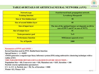
TABLE 68 DETAILSOF ARTIFICIALNEURAL NETWORK (ANN)
Network type Feed-forward back propagation network
Training function Levenberg-Marquardt
Size of first hidden layer 50
Size of second hidden layer 05
Size of input layer The size of the optimal feature set depends on (04 in
case of DWT and 07 in case of WPT)
Size of output layer 01
Train parameter goal 7e-9
Performance function MSE(mean squared error)
No. of Epochs 1000
88/93
Parameters of PNN and ANFIS :
Kernel function used in PNN: Radial basis function
Spread factor () = 0.025
ANFIS generates a sugeno-type fuzzy inference system (FIS) using subtractive clustering technique with a
radius of 0.5.
THE PARAMETERS DETAILS OF GA BASED FEATURE SELECTION :
Population Size = 60, Cross-over rate = 0.8, Mutation rate = 0.01. Iteration = 100
Particle swarm optimization parameters
C1= 4, C2= 4, Particle size = 50, No. of iteration = 1000
Wmin= 0.5, Wmax= 0.9
89.
REFERENCES
1. Liao, Y.(2008) Generalized fault-location methods for overhead electric distribution systems , IEEE Trans Power
Deliv , 26 (1). pp.53–64.
2. Krishnathevar, R. (2012) Generalized impedance-based fault location for distribution systems. IEEE Trans Power
Del , 27 (1) pp.449–51.
3. Samantaray, S. R.; Dash P. K. (2007) Wavelet packet based digital relaying for advanced series compensated line, IET
Gener. Transm. Distrib., vol. 1, no. 5, pp. 784-793.
4. Capar, A.; Arsoy, A. B. (2015) A performance oriented impedance based fault location algorithm for series
compensated transmission lines, Electrical Power and Energy Systems 71 pp. 209–214.
5. Eriksson, L.; Saha, M.; Rockefeller, G D. (1985) An accurate fault locator with compensation for apparent reactance
in the fault resistance resulting from the remote - end feed, IEEE transactions on Power Apparatus and Systems, 104:
pp.424–436.
6. Dong, X.; Kong, W.; and Cui, T. (2009) Fault classification and faulted phase selection based on the initial current
travelling wave,” IEEE Trans. Power Del., vol. 24, issue. 2, pp. 552-559.
7. Shehab-Eldin, E. H.; McLaren, P. G. (1998) Travelling wave distance protection-problem areas and solutions , IEEE
Trans. Power Del., vol. 3, issue. 3, pp. 894-902.
8. Ngu, E. E.; and Ramar, K. (2011) A combined impedance and travelling wave based fault location method for multi-
terminal transmission lines, Int. Journal of Electric Power and Energy Systems, vol. 33, issue. 10, pp. 1767-1775.
9. Das, R.; Sachdev M.; and Sidhu, T. (2000) A fault locator for radial subs transmission and distribution lines, IEEE
Power Eng. Soc. Summer Meeting, Seattle, vol. 1, pp. 443-448.
10. Aggarwal, R. K.; Aslan, Y.; Johns, A. T. (1997) “New concept in fault location for overhead distribution systems
using superimposed components”, IET Gener. Transm. Distrib., vol. 144, issue.3, pp. 309-316.
11. Rui, L.; Guoqing, F.; Xueyuan, Z.; Xue, X. (2015) Fault location based on single terminal travelling wave analysis in
radial distribution network, Electrical Power and Energy Systems, 66 , pp.160–165
12. Teng, J. H.; Huang, W.-H.; Luan, S.W. (2014) Automatic and Fast Faulted Line-Section Location Method for
Distribution Systems Based on Fault Indicators, IEEE Transactions on Power systems, vol. 29, no. 4, pp. 1653-1662.
13. Brahma, S. M. (2011) Fault location in power distribution system with penetration of distributed generation,
IEEE Trans. Power Del., vol. 26, issue. 3, pp. 1545-1553.
14. Yang, X.; Choi, M.; Lee, S.; Ten, C.; Lim, S. (2008) Fault location for underground power cable using distributed
parameter approach, IEEE Trans. Power System, vol. 23, issue. 4, pp. 1809-1816. 89/93
90.
REFERENCES
15. Gururajapathy, S.S.;Mokhlis, H.; Illias, H.A. (2017) Fault location and detection techniques in power
distribution systems with distributed generation: A review, Renewable and Sustainable Energy Reviews 74, 949–
958.
16. Samantaray, S. R.; Dash P. K.; Panda, G. (2006) Fault classification and location using HS-transform and radial
basis function neural network, Electric power system research, vol. 76, Issue 9-10, pp. 897-905.
17. Silva, K. M.; B. A. Souza, Brito, N. S. D. (2006) Fault Detection and Classification in Transmission Lines Based
on Wavelet Transform and ANN, IEEE Transactions on Power Delivery, vol. 21, no. 4, pp.2058-2063.
18. 13. Goudarzi, M.; Vahidi, B.; Naghizadeh R. A.; Hosseinian, S. H. (2015) Improved fault location algorithm for
radial distribution systems with discrete and continuous wavelet analysis, Electrical Power and Energy Systems,
vol. 67, pp. 423-430.
19. Stockwell, R. G.; Mansinha, L.; Lowe, R. P. (1996) Localization of the complex spectrum: the S transform , IEEE
Transactions on Signal Processing; 44: 998-1001.
20. Ray, P.; Panigrahi, B. K.; Senroy, N. (2013) Hybrid methodology for fault distance estimation in series
compensated transmission line. IET Gen. Trans. Dist., 7 (5): pp. 431-439.
21. Chandrashekar , G.; Sahin, F. (2014) A survey on feature selection methods, Computers and Electrical
Engineering, 40, pp.16–28
22. Devroye, L. (1978) The uniform convergence of nearest neighbor regression function estimators and their
application in optimization, IEEE Transactions on Information Theory, 24: pp.142-151.
23. Navot, A.; Shpigelman, L.; Tishby, N.; Vaadia, E. (2006) Nearest neighbor based feature selection for regression
and its application to neural activity, In Proceedings of the International Conference on Advances in neural
information processing systems (NIPS) , 18: pp.995-1002.
24. Molina, L. C.; Belanche L.; Nebot, A. (2003) Feature selection algorithms: a survey and experimental evaluation,
in: Proceedings of the IEEE on Data Mining (ICDM), pp.306-313.
25. Ghamisi, P.; and Benediktsson, J. A. (2015) Feature Selection Based on Hybridization of Genetic Algorithm and
Particle Swarm Optimization, IEEE Geoscience and Remote Sensing Letters, vol. 12, no. 2, february , pp. 309-
313.
26. Xue, B.; Zhang, M.; Browne, W. N. (2013) Particle Swarm Optimization for Feature Selection in Classification:
A Multi-Objective Approach, IEEE Transactions on Cybernetics, vol. 43, no. 6, pp. 1656-1670.
27 Huang , C. L.; Wang , C. J. (2006) A GA-based feature selection and parameters optimization for support vector
machines, Expert Systems with Applications ,31, pp. 231–240 90/93
91.
REFERENCES
28. Ekici, S.;Yildirum, S.; Poyraz, M. (2008) Energy and entropy based feature extraction for locating fault on
transmission lines by using neural network and wavelet packet decomposition, Expert systems with
application, vol. 34, pp. 2937-2944.
29. Zhanga, J. R.; Zhanga, J.; Lokc, T.M.; Lyud, M. R. (2007) A hybrid particle swarm optimization–back-
propagation algorithm for feedforward neural network training , Applied Mathematics and Computation ,
Volume 185, Issue 2, 15, pp. 1026–1037
30. Mao, K. Z.; Tan K. C.; Ser, W. (2000) Probabilistic neural network structure determination for pattern
classification, IEEE Trans. Neural Networks, vol. 11, issue. 4, pp. 1009-1016
31. Reddy, M.J.; Mohanta, D.K. (2008) Adaptive-neuro-fuzzy inference system approach for transmission line fault
classification and location incorporating effects of power swings, IET Gener. Transm. Distrib., 2 (2), pp. 235–244
32. Ekici, S. (2012) Support vector machines for fault classification and locating faults on transmission lines,
Applied soft computing, vol. 12, issue. 6, pp. 1650-1658.
33. Malathi, V.; Marimuthu, N. S.; Baskar, S. (2010) Intelligent approaches using support vector machine and
extreme learning machine for transmission line protection, Journal of Neurocomputing, vol. 73, pp. 2160-2167.
34. Sadeh, J.; Hadjsaid, N.; Ranjbar, A. M.; Feuillet, R. (2000) Accurate fault location algorithm for series
compensated transmission lines, IEEE Trans. Power Del. 15 (3): pp.1027-1033.
35. Malathi, V. N.; Marimuthu, S.; Baskar S.; Ramar, K. (2011) Application of extreme learning machine for series
compensated transmission line protection, Engineering Applications of Artificial Intelligence, vol. 24(5) pp. 880-
887.
36. Dash, P. K.; Samantaray, S. R.; Panda, G. (2007) Fault classification and section identification of an advanced
series compensated transmission line using support vector machine. IEEE Trans. Power Del., 22:pp. 67-73.
37. Sahoo, S.; Ray, P.; Panigrahi, B. K.; Senroy, N. (2010) A computational intelligence approach for fault location in
transmission lines, In: Proc., IEEE conf. Power electronics, Drives and Energy systems (PEDES-2010), Dec. 21-
23, pp. 1-6.
38. Saha, M. M.; Izykowski, J.; Rosolowski, E.; Kasztenny, B. (1999) A new accurate fault locating algorithm for
series compensated lines, IEEE Trans. Power Del., 14 (3): pp.789-797.
39. Jamila, M.; Kalama, A.; Ansaria, A. Q.; Rizwanb, M. (2014) Generalized neural network and wavelet transform
based approachfor fault location estimation of a transmission line Applied Soft Computing 19, 322–332
91/93
92.
REFERENCES
40. Parikh, U.;Das, B.; Maheshwari, R. (2008) Combined Wavelet-SVM Technique for Fault Zone Detection in a Series
Compensated Transmission Line, IEEE Transaction in Power Delivery, 23(4), pp. 1789-1794.
41. Dash, P. K.; Samantaray, S. R.; Panda, G. (2007) Fault classification and section identification of an advanced series
compensated transmission line using support vector machine. IEEE Trans. Power Del., 22:pp. 67-73.
42. Samantaray, S.R. (2009) Decision tree-based fault zone identification and fault classification in flexible AC
transmissions-based transmission line, IET Gener. Transm. Distrib., Vol. 3, Iss. 5, pp. 425–436
43. Dash, P. K.; Chilukuri, M. V. (2003) Soft Computing Tools for Protection of Compensated Network National Power
and Energy Conference (PECon) Proceedings, Bangi, Malaysia pp. 52-61
44. Meyar-Naimi, H (2012) A new fuzzy fault locator for series compensated transmission lines, IEEE 11th International
Conference on Environment and Electrical Engineering , Venice, pp. 53-58.
45. Rajeswary, G. R.; Kumar G. R.; Lakshmi, G. J. S.; Anusha, G. (2016) Fuzzy-Wavelet Based Transmission Line
Protection Scheme In The Presence Of TCSC, International Conference on Electrical, Electronics, and Optimization
Techniques.
46. Lovisolo, L.; Moor Neto, J.A.; Figueiredo, K. ; Menezes Laporte, L. d. ; Santos Rocha, J.C. d. (2012) Location of
faults generating short-duration voltage variations in distribution systems regions from records captured at one point
and decomposed into damped Sinusoids, IET Gener. Transm. Distrib., Vol. 6, Iss. 12, pp. 1225–1234
47. Oliveira, A. R.; Garcia, P. A. N.; Oliveira, L. W.; Pereira, J. L. R.; Silva, H. A.
(2011) Distribution system to fault classification using negative sequence and intelligent system, 16th International
Conference on Intelligent System Application to Power Systems .
48. Salim, R. H.; Oliveira, K. R. C. D.; Filomena, A. D.; Resener, M.;0 Bretas, A. S.
(2008) Hybrid Fault Diagnosis Scheme Implementation for Power Distribution Systems Automation IEEE
Transactions on power delivery, vol. 23, no. 4, 2008 pp 1846-1856
49. Dashti, R.; Sadeh, J. (2013) Applying Dynamic Load Estimation and Distributed-parameter Line Model to Enhance
the Accuracy of Impedance-based Fault-location Methods for Power Distribution Networks, Electric Power
Components and Systems, 41, pp. 1334–1362.
50. Lee, S. J.; Choi, M. S. ; Kang, S. H.; Jin, B. G.; Lee, D. S.; Ahn, B. S.; Yoon, N. S.; Kim, H. Y.; Wee, S. B. (2004) An
Intelligent and Efficient Fault Location and Diagnosis Scheme for Radial Distribution Systems, IEEE Transactions on
Power delivery, vol. 19, no. 2. 92/93
93.
REFERENCES
51. Resener ,M.; Salim, R. H.; Filomena, A. D.; Bretas, A. S. (2008) “Optimized fault location formulation for unbalanced distribution
feeders considering load variation, 16th PSCC, Glasgow, Scotland, pp. 1-7
52. Nunes, J. U. N.; Bretas, A. S. (2011) A impedance-based fault location technique for unbalanced distributed generation systems, in proc.
2011 IEEE Trondheim Power Tech, pp. 1-7.
53. Bretas, A.S.; Salim, R. H. (2006) Fault Location in Unbalanced DG Systems using the Positive Sequence Apparent Impedance, in proc.
IEEE Transmission and Distribution Conference and Exposition: Latin America, pp.1-6.
54. Nunes, J.U.N.; Bretas, A.S. (2010) Impedance-based fault location formulation for unbalanced primary distribution systems with
distributed generation, in proc. International Conference on Power System Technology , pp.1-7.
55. Adewole , A. C.; Tzoneva, R. (2012) Fault Detection and Classification in a Distribution Network Integrated with Distributed Generators,
IEEE/ PES Power Africa Conference and Exhibition Johannesburg, South Africa.
56. Nauman, S.; Aleem, S. A.; Haider, N. I.; Zaffar, N. (2012) Support vector machine based fault detection & classification in smart grids, In
Globecom workshops (GC wkshps. IEEE; ) pp. 1526–31.
57. Rafinia, A.; Moshtagh, J. (2014) A new approach to fault location in three-phase underground distribution system using combination of
wavelet analysis with ANN and FLS Electrical Power and Energy Systems, 55, pp. 261–274
58. Gilany , M.; Ibrahim , D. K.; Sayed , T. E. El. (2007) Traveling wave based fault location scheme for multi end aged underground cable
system, IEEE Transaction on Power. Del. 22(1) pp. 82–89.
59. Yoomak, S.; Pothisarn, C.; Jettanasen, C.; Ngaopitakkul A. (2017) Discrete Wavelet Transform and Fuzzy Logic Algorithm for
Classification of Fault Type in Underground Cable, Advances in Fuzzy Logic and Technology , pp 564-573
60. Sidhu, T. S.; Xu, Z. (2009) Detection and classification of incipient faults in underground cables in distribution systems, Canadian
Conference on Electrical and Computer Engineering.
61. Niazy, I.; Sadeh, J. (2013) A new single ended fault location algorithm for combined transmission line considering fault clearing transients
without using line parameters, Electrical Power and Energy Systems, 44 pp.816–823.
62. Ngaopitakkul, A.; Suttisinthong, N. (2012) Discrete wavelet transform and probabilistic neural network algorithm for classification of
fault type in underground cable, Proceedings of the International Conference on Machine Learning and Cybernetics, Xian.
63. Klomjit, J.; Ngaopitakkul , A. (2017) Fault Classification on the Hybrid Transmission Line System Between Overhead Line and
Underground Cable, IFSA-SCIS 2017, Otsu, Shiga, Japan.
64. Livani, H.; Evrenosoğlu, C. Y. (2012) A Fault Classification Method in Power Systems Using DWT and SVM Classifier, IEEE PES
Transmission and Distribution Conference and Exposition.
65. Han, J.; Crossley, P.A. (2014) Fault Location on a Mixed Overhead and Underground Transmission Feeder Using a Multiple-Zone
Quadrilateral Impedance Relay and a Double-ended Travelling Wave Fault Locator , 12th IET
International Conference on Developments in Power System Protection .
66. Ferreira, G. D.; Gazzana, D. d. S.; Bretas, A. S.; Ferreira, A. H.; Bettiol, A. L.; Carniato, A. (2012) Impedance-Based Fault Location for
Overhead and Underground Distribution Systems, North American Power Symposium , pp.1-6
67. Niazy, I.; Sadeh, J. (2013) A new single ended fault location algorithm for combined transmission line considering fault clearing transients
without using line parameters, Electrical Power and Energy Systems 44 pp. 816–823
94.
LIST OF SOMESELECTED PUBLICATIONS
1. P. Ray, S. R. Arya, D. P. Mishra, “Intelligence Scheme for fault location in a combined overhead transmission line &underground cable,” International Journal of
Emerging Electric Power Systems. Vol 19, Issue 5, 2018, pp. 1-18, DOI: 10.1515/ijeeps-2017-0277 (DE GRUYTER, Scopus, ESCI, IF-1) ISSN: 1553-779X
2. D. P. Mishra and P. Ray, “Fault detection, location and classification of a transmission line,” Neural Computing and Applications, Vol. 30, 2018, No. 5,pp. 1377-
1424. DOI 10.1007/s00521-017-3295-y (Springer)(SCI, IF-6) ISSN: 09410643, 14333058
3. P. Ray and D. P. Mishra, “Support Vector Machine Based Fault Classification and Location of a Long Transmission Line”, Engineering Science and Technology, an
International Journal 19 (2016) pp.1368–1380. https://doi.org/10.1016/j.jestch.2016.04.001. (Elsevier) (SCI, Scopus, IF-5.7), Online ISSN: 2215-0986
4. P. Ray and D. P. Mishra, “Application of extreme learning machine for underground cable fault location,” International Transactions on Electrical Energy Systems,
vol. 25, Issue. 12, Dec. 2015, pp. 3227–3247.(Willy) (SCI, IF-2.3), https://doi.org/10.1002/etep.2032 Online ISSN:2050-7038 , Print ISSN:2050-7038
5. S. K. Panda, P. Ray, and D. P. Mishra, “ An Efficient Short-Term Electric Power Load Forecasting Using Hybrid Techniques," International Journal of Computer
Information Systems and Industrial Management Applications, Volume 12 , pp. 387-397 , Nov., 2020. (Scopus, , SJR: 0.16)
6. S. R. Das, D. P. Mishra, P. K. Ray, S. R. Salkuti, A. K. Sahoo, " Power Quality Improvement using Fuzzy Logic Based Compensation in a Hybrid Power System,"
International Journal of Power Electronics and Drive System (IJPEDS), Vol. 11, No. 3, Dec 2020, (Scopus, CiteScore: 1.49, SJR: 0.304)
7. A. P. Hota, S. Mishra, D. P. Mishra, S. R. Salkuti, “ Allocating active power loss with network reconfiguration in electrical power distribution systems,"
International Journal of Power Electronics and Drive System (IJPEDS), Vol. 11, No. 3, Dec 2020, (Scopus, CiteScore: 1.49, SJR: 0.304)
8. S. R. Das, P. K. Ray, D. P. Mishra, H. Das, “Performance assessment of PV integrated Model Predictive Controller based hybrid filter for Power Quality
Improvement”, International Journal of Power Electronics, 2020. (Inder science, Scopus, SJR-0.14)
94/93
95.
LIST OF SOMESELECTED PUBLICATIONS
1. PAPERS PUBLISHED IN INTERNATIONAL CONFERENCE
1. S. Jena, D. P. Mishra, S. R. Salkuti, (2023). Fault Detection, Classification, and Location in Underground Cables. In: Salkuti, S.R., Ray, P., Singh, A.R. (eds) Power Quality in Microgrids: Issues,
Challenges and Mitigation Techniques. Lecture Notes in Electrical Engineering, vol 1039. Springer, Singapore. https://doi.org/10.1007/978-981-99-2066-2_10, Publisher Name: Springer, Singapore, Print
ISBN:978-981-99-2065-5, Online ISBN:978-981-99-2066-2, pp 195-215.
2. Mishra, D.P., Biswal, P., Sahu, S.S., Dash, S., Giri, N.C. (2023). Radial Basis Function Neural Network with Wavelet Transform for Fault Detection in Transmission Line. In: Rani, A., Kumar, B.,
Shrivastava, V., Bansal, R.C. (eds) Signals, Machines and Automation. SIGMA 2022. Lecture Notes in Electrical Engineering, vol 1023. Springer, Singapore.
https://doi.org/10.1007/978-981-99-0969-8_9, Publisher Name: Springer, Singapore, Print ISBN 978-981-99-0968-1,Online ISBN 978-981-99-0969-8
3. S. Jena, D. P. Mishra and S. Mishra, "Detection and Classification of Permanent Fault Using Multi-Layer Perceptron Model in a Distribution Network," 2023 IEEE 3rd International Conference on Smart
Technologies for Power, Energy and Control (STPEC), Bhubaneswar, India, 2023, pp. 1-6, doi: 10.1109/STPEC59253.2023.10431048. Date: 10th-13th December 2023 Electronic ISBN:979-8-3503-
0473-2, Physical presentation
4. Panda S.K., Ray P., Mishra D.P. (2021) A Study of Machine Learning Techniques in Short Term Load Forecasting Using ANN. In: Mishra D., Buyya R., Mohapatra P., Patnaik S. (eds) Intelligent and
Cloud Computing. Smart Innovation, Systems and Technologies, vol 194. Springer, Singapore. https://doi.org/10.1007/978-981-15-5971-6_6
5. M. A. R. Tilak, U. Subudh, D. P. Mishra, “Performance Analysis of Lead Acid Batteries with the Variation of Load Current and Temperature,” Advances in Smart Grid and Renewable Energy. ETAEERE
2020. Lecture Notes in Electrical Engineering, vol 691. Springer, Singapore., March 2020, pp. 15-23 https://doi.org/10.1007/978-981-15-7511-2_2
6. S. K. Panda, P. Ray, D. P. Mishra,“ A Study of Machine Learning Techniques in Short Term Load Forecasting Using ANN”, Intelligent and Cloud Computing. Smart Innovation, Systems and
Technologies, vol 194. Springer, Singapore. https://doi.org/10.1007/978-981-15-5971-6_6, Dec, 2019.pp.49-57
7. P. Mohanty, D. P. Mishra, A.Behera, Swati Swarupa Das, “Demonstration and Simulation of Brushless Direct Current Motor,” Advances in Energy Technology Proceedings of ICAET 2020, Jan. 2020, pp
79-89. Jan. 2020 pp.1-9
8. R. Mishra, D. P. Mishra, “Comparison of neural network models for weather forecasting,” Advances in Energy Technology Proceedings of ICAET 2020, Jan. 2020, pp. 79-89.
9. Papia Ray, D. P. Mishra, “Introduction to Condition Monitoring of Wide Area Monitoring (WAM) System,” Chapter 4 of the book Titled Soft Computing In Condition Monitoring And Diagnostics Of
Electrical And Mechanical Systems. (Springer) 2020, pp.71-89.(Springer S. K. Panda, P. Ray, D. P. Mishra, “A Review on ANN In Short Term Load Forecasting Using Artificial Intelligence Techniques”,
International Conference on Intelligent and cloud computing (ICICC-2019), to be held at ITER, SOA university, from 16-17 Dec, 2019. (Springer)
10. A. P. Hota, S. K. Mishra and D. P. Mishra,” Loss allocation strategies in active power distribution networks: A review, 1st international conference on advances in electrical control & signal systems
(AECSS-2019)” to be held at ITER, SOA, from Nov 8-9, 2019, (Springer)
11. A. P. Hota, S. K. Mishra and D. P. Mishra, “A new active power loss allocation method for radial distribution networks with DGs.” 1st international conference on advances in electrical control & signal
systems (AECSS-2019)” to be held at ITER, SOA, from Nov 8-9, 2019, (Springer)
12. S. K. Panda, P. Ray, D. P. Mishra, “Effectiveness of PSO On Short Term Load Forecasting,” 1st International Conference on Application of Robotics in Industry using Advanced Mechanisms, August,
16-17, 2019, GIFT, Bhubaneswar, India,PP. (Springer)
13. P. Ray, D. P. Mishra, “Analysis of EEG Signals for Emotion Recognition using Different Computational Intelligence Techniques”, Applications of Artificial Intelligence Techniques in Engineering.
SIGMA 2018, Volume 2. Advances in Intelligent Systems and Computing, vol 697. Springer, Singapore, pp 527-536 (Springer)
95/93
#8 in case of series compensated transmission line with capacitor placed at the middle, impedance based algorithms suffers from the draw back as the impedance seen by the relay is same for faults before and after the capacitor which make it difficult to locate the fault properly. However, in AI methods which uses transient information available on the signal, this problem is overcome as the transients those appears in the faulty signal are different for the fault before and after the capacitor in the transmission line and the transient frequencies are different if the fault path is having capacitor in comparison to the fault path without capacitor.
#15 A new fault location scheme for power transmission line is proposed in this paper. The simulations show that, the scheme has a
high accuracy for estimation of fault locations using 1/2 circle post fault phase voltage measurements. All the 11 types of faults at different inception angles on a 285.65 km long power transmission line system were used. Compared with other methods, the scheme in this paper needs less information and short time data window to estimate fault location. The scheme only used 1/2 cycle to accurately decide where a fault has occurred along the transmission line. It indicates that the scheme proposed in this paper can correctly and rapidly locate the faults with different fault type and different fault inceptions. We also observed that using a low pass filter, improved the accuracy of the scheme.
#17 The proposed algorithm is independent of steady state information and apparent impedance of the fault signal. Impedance based algorithms suffer from this draw back as the impedance seen by the relay is same for faults before and after TCSC. As this particular adopted method is based on the transient information available on the signal, the transients those appear in the faulty signal are different for the fault before and after TCSC. The transient frequencies are different if the fault path is having TCSC in comparison to the fault path without TCSC.
#18
Computational model, simulates the structure and functional aspects of biological neural network , approach similar to human brain to make decision and to arrive at conclusions.
Multi-layered feedforward neural network (MLFNN) with backpropagation training algorithm.
Input layer, two hidden layer, output layer
Simplicity and good generalization
Performance function is mean square error (MSE)
Neural network refers to a network or circuit of interconnected biological neuron
An artificial neural network (ANN) is a computational model that tries to simulate the structure and functional aspects of biological neural network and uses an approach similar to human brain to make decision and to arrive at conclusions.
A learning rule is a procedure to modify the weights of the nn and a perceptron is a architecture of single layer of neuron and it performs transformation of linear combination of inputs. Here supervised learning is used which is adaptive (able to change the weights).
MLFNN is used for its simplicity and good generalisation. It consists on input layer, hidden layer and one output layer.
For improving the performance and to adjust the connection between the layers, information about the errors is filtered back through the system. Forward pass and backward pass are the two passes through the different layers of the network for the error back propagation process. An activation pattern is applied to the nodes of the network in the forward pass and its effect propagates through the network layer by layer. Output set produced is the actual response of the network. To produce error signal, the actual response of the network is subtracted from the desired signal. This error signal is propagated backward through the network against the direction of synaptic weight connections and the synaptic weights are adjusted to make actual response of the network much closer to the desired response.
Transfer func. Is sigmiodal. Sigmoidal means output varies continuously but not linearly as input.
#19
Computational model, simulates the structure and functional aspects of biological neural network , approach similar to human brain to make decision and to arrive at conclusions.
Multi-layered feedforward neural network (MLFNN) with backpropagation training algorithm.
Input layer, two hidden layer, output layer
Simplicity and good generalization
Performance function is mean square error (MSE)
Neural network refers to a network or circuit of interconnected biological neuron
An artificial neural network (ANN) is a computational model that tries to simulate the structure and functional aspects of biological neural network and uses an approach similar to human brain to make decision and to arrive at conclusions.
A learning rule is a procedure to modify the weights of the nn and a perceptron is a architecture of single layer of neuron and it performs transformation of linear combination of inputs. Here supervised learning is used which is adaptive (able to change the weights).
MLFNN is used for its simplicity and good generalisation. It consists on input layer, hidden layer and one output layer.
For improving the performance and to adjust the connection between the layers, information about the errors is filtered back through the system. Forward pass and backward pass are the two passes through the different layers of the network for the error back propagation process. An activation pattern is applied to the nodes of the network in the forward pass and its effect propagates through the network layer by layer. Output set produced is the actual response of the network. To produce error signal, the actual response of the network is subtracted from the desired signal. This error signal is propagated backward through the network against the direction of synaptic weight connections and the synaptic weights are adjusted to make actual response of the network much closer to the desired response.
Transfer func. Is sigmiodal. Sigmoidal means output varies continuously but not linearly as input.
#20
Computational model, simulates the structure and functional aspects of biological neural network , approach similar to human brain to make decision and to arrive at conclusions.
Multi-layered feedforward neural network (MLFNN) with backpropagation training algorithm.
Input layer, two hidden layer, output layer
Simplicity and good generalization
Performance function is mean square error (MSE)
Neural network refers to a network or circuit of interconnected biological neuron
An artificial neural network (ANN) is a computational model that tries to simulate the structure and functional aspects of biological neural network and uses an approach similar to human brain to make decision and to arrive at conclusions.
A learning rule is a procedure to modify the weights of the nn and a perceptron is a architecture of single layer of neuron and it performs transformation of linear combination of inputs. Here supervised learning is used which is adaptive (able to change the weights).
MLFNN is used for its simplicity and good generalisation. It consists on input layer, hidden layer and one output layer.
For improving the performance and to adjust the connection between the layers, information about the errors is filtered back through the system. Forward pass and backward pass are the two passes through the different layers of the network for the error back propagation process. An activation pattern is applied to the nodes of the network in the forward pass and its effect propagates through the network layer by layer. Output set produced is the actual response of the network. To produce error signal, the actual response of the network is subtracted from the desired signal. This error signal is propagated backward through the network against the direction of synaptic weight connections and the synaptic weights are adjusted to make actual response of the network much closer to the desired response.
Transfer func. Is sigmiodal. Sigmoidal means output varies continuously but not linearly as input.
#21
Computational model, simulates the structure and functional aspects of biological neural network , approach similar to human brain to make decision and to arrive at conclusions.
Multi-layered feedforward neural network (MLFNN) with backpropagation training algorithm.
Input layer, two hidden layer, output layer
Simplicity and good generalization
Performance function is mean square error (MSE)
Neural network refers to a network or circuit of interconnected biological neuron
An artificial neural network (ANN) is a computational model that tries to simulate the structure and functional aspects of biological neural network and uses an approach similar to human brain to make decision and to arrive at conclusions.
A learning rule is a procedure to modify the weights of the nn and a perceptron is a architecture of single layer of neuron and it performs transformation of linear combination of inputs. Here supervised learning is used which is adaptive (able to change the weights).
MLFNN is used for its simplicity and good generalisation. It consists on input layer, hidden layer and one output layer.
For improving the performance and to adjust the connection between the layers, information about the errors is filtered back through the system. Forward pass and backward pass are the two passes through the different layers of the network for the error back propagation process. An activation pattern is applied to the nodes of the network in the forward pass and its effect propagates through the network layer by layer. Output set produced is the actual response of the network. To produce error signal, the actual response of the network is subtracted from the desired signal. This error signal is propagated backward through the network against the direction of synaptic weight connections and the synaptic weights are adjusted to make actual response of the network much closer to the desired response.
Transfer func. Is sigmiodal. Sigmoidal means output varies continuously but not linearly as input.
#23 the cycle of the current and voltage signal was taken for analysis after the inception of fault at a sampling frequency of 30 kHz. The measured signals were decomposed to 8-levels by DWT.
2. Thereafter features were extracted from the decomposed signal. Six features (as mentioned in section III) were extracted for each of the sub band.
3.
#37 Supervised learning tasks are represented by large feature set as input, out of which many are redundant. The method which removes the redundant features and makes the feature set optimal is called feature selection. These optimal features predict the target properly and enhance the accuracy.
1. In machine learning, stepwise regression is a popular feature selection technique which is a greedy algorithm. A greedy algorithm solves any regression related problem very quickly by making the locally optimal choice at each step and is computationally advantageous and robust against overfitting. Forward feature selection is one such greedy algorithm.
2. An evaluation function is used to assign scores to features and a search algorithm is used to search for a subset with a high score. The evaluation function used in this paper is leave one out (LOO) mean square error (MSE) of the k-nearest-neighbor (KNN) estimator which gives a good approximation of the expected generalization error.
3. The KNN estimator is defined as the weighted average of nearest neighbor, where the weight of each neighbor is proportional to its proximity .
4. evaluation function e (w) is defined as the negative (halved) MSE of weighted KNN estimator.
#38 stochastic optimization based technique inspired by the behavior of bird flocking or fish schooling.
In PSO, the potential solution is called particles, which interacts among themselves to find global optimal solution.
At every step of iteration, each particle has its own position and velocity and is updated by two best values (fitness) called as pbest and gbest.
Pbest is defined as the best solution achieved in every step of the iteration process so far and the gbest is the best solution obtained so far by any particle in the population. After finding these two best values, particle updates its position and velocity.
position of the particle is assigned one if the fitness function of the particle is greater than the randomly generated number and chosen for the next level, otherwise it is assigned zero and discarded.
Algorithm is:-
Step 1. Initialize the training data set
Step 2. Calculate velocity and position for each particle .
Step 3. Calculate the fitness function of each particle .
Step 4. Calculate pbest and gbest
Step 5. Update new position and new velocity of the particle
Step 6. Check whether the fitness function of the new updated particle is greater than a random number
Step 7. If yes, then that particle is chosen.
(position of the particle is assigned one if the fitness function of the particle is greater than the randomly generated number and chosen for the next level, otherwise it is assigned zero and discarded).
Step 8. Go to next generation until stopping criteria is met.
#40 Support vector machine is an adaptive computational learning technique based on statistical learning theory in which the original input vectors are nonlinearly mapped into a high dimensional feature space and the optimal hyper plane is determined to maximize the generalization ability
LIBSVM.
Overfitting occurs when a model fail to generalize.It depends on no. of parameters and data, conformability of the model structure to the data shape, magnitude of model error compared to the error in the data or level of noise. To avoid it crossvalidation or regularization is performed.
regularization involves introducing additional information in order to solve an ill-posed problem or to prevent overfitting. This information is usually of the form of a penalty for complexity, such as restrictions for smoothness or bounds on the vector space norm.
Example of regularization is least square method.In SVM L2 norm is used. a norm is a function that assigns a strictly positive length or size to all vectors in a vector space, other than the zero vector (which has zero length assigned to it).
If the training error decreases (negative slope) while the validation error increases (positive slope),then overfitting has occurred.
#41 It is the process of choosing a small subset from all the features that is sufficient to predict the target properly. It helps in reducing the computational complexity of learning and prediction algorithms and enhances the prediction accuracy.
It helps in reducing the computational complexity of learning and prediction algorithms and enhances the prediction accuracy.
This method operates with a set of population of chromosome represented by a string of binary digits and each chromosome is selected for the next generation on the basis of a fitness function which is used to evaluate the quality of each chromosome.
one of the features from the available six features is selected from all the DWT decomposition by GA encoding scheme and each coefficient is represented by six binary digit.
Three basic steps in this method are reproduction, crossover and mutation. A ranking method is used for the reproduction of the chromosome set in which an entire set of chromosomes gets a rank based on the fitness function and the selection of chromosomes is done based on the highest ranking.
After that a crossover operation is performed in which to produce a child chromosome, more than one parent chromosome is considered. A uniform crossover is used with a 0.5 mixing ratio between the two parents so that the child chromosome gets approximately half of the genes from one parent and another half from the other with the crossover point(mask) randomly chosen.
To maintain diversity within a string of chromosomes, a mutation operation is then performed which randomly alters the bit of the chromosome string with a probability of 0.001.
The advantage of this method over other conventional techniques of feature selection is that it works well with large feature set and has less chance to converge into local optimal solution.
#42 It is the process of choosing a small subset from all the features that is sufficient to predict the target properly. It helps in reducing the computational complexity of learning and prediction algorithms and enhances the prediction accuracy.
It helps in reducing the computational complexity of learning and prediction algorithms and enhances the prediction accuracy.
This method operates with a set of population of chromosome represented by a string of binary digits and each chromosome is selected for the next generation on the basis of a fitness function which is used to evaluate the quality of each chromosome.
one of the features from the available six features is selected from all the DWT decomposition by GA encoding scheme and each coefficient is represented by six binary digit.
Three basic steps in this method are reproduction, crossover and mutation. A ranking method is used for the reproduction of the chromosome set in which an entire set of chromosomes gets a rank based on the fitness function and the selection of chromosomes is done based on the highest ranking.
After that a crossover operation is performed in which to produce a child chromosome, more than one parent chromosome is considered. A uniform crossover is used with a 0.5 mixing ratio between the two parents so that the child chromosome gets approximately half of the genes from one parent and another half from the other with the crossover point(mask) randomly chosen.
To maintain diversity within a string of chromosomes, a mutation operation is then performed which randomly alters the bit of the chromosome string with a probability of 0.001.
The advantage of this method over other conventional techniques of feature selection is that it works well with large feature set and has less chance to converge into local optimal solution.
#43 In this work, GA encoding scheme selects one of the feature from the available six features in all 16 coefficients of the 4th level of WPT decomposition and each parameter is represented by 6 binary digit.
In this case, optimal features are selected during training.
#44
Computational model, simulates the structure and functional aspects of biological neural network , approach similar to human brain to make decision and to arrive at conclusions.
Multi-layered feedforward neural network (MLFNN) with backpropagation training algorithm.
Input layer, two hidden layer, output layer
Simplicity and good generalization
Performance function is mean square error (MSE)
Neural network refers to a network or circuit of interconnected biological neuron
An artificial neural network (ANN) is a computational model that tries to simulate the structure and functional aspects of biological neural network and uses an approach similar to human brain to make decision and to arrive at conclusions.
A learning rule is a procedure to modify the weights of the nn and a perceptron is a architecture of single layer of neuron and it performs transformation of linear combination of inputs. Here supervised learning is used which is adaptive (able to change the weights).
MLFNN is used for its simplicity and good generalisation. It consists on input layer, hidden layer and one output layer.
For improving the performance and to adjust the connection between the layers, information about the errors is filtered back through the system. Forward pass and backward pass are the two passes through the different layers of the network for the error back propagation process. An activation pattern is applied to the nodes of the network in the forward pass and its effect propagates through the network layer by layer. Output set produced is the actual response of the network. To produce error signal, the actual response of the network is subtracted from the desired signal. This error signal is propagated backward through the network against the direction of synaptic weight connections and the synaptic weights are adjusted to make actual response of the network much closer to the desired response.
Transfer func. Is sigmiodal. Sigmoidal means output varies continuously but not linearly as input.
#47 Support vector machine is an adaptive computational learning technique based on statistical learning theory in which the original input vectors are nonlinearly mapped into a high dimensional feature space and the optimal hyper plane is determined to maximize the generalization ability
LIBSVM.
Overfitting occurs when a model fail to generalize.It depends on no. of parameters and data, conformability of the model structure to the data shape, magnitude of model error compared to the error in the data or level of noise. To avoid it crossvalidation or regularization is performed.
regularization involves introducing additional information in order to solve an ill-posed problem or to prevent overfitting. This information is usually of the form of a penalty for complexity, such as restrictions for smoothness or bounds on the vector space norm.
Example of regularization is least square method.In SVM L2 norm is used. a norm is a function that assigns a strictly positive length or size to all vectors in a vector space, other than the zero vector (which has zero length assigned to it).
If the training error decreases (negative slope) while the validation error increases (positive slope),then overfitting has occurred.
#49 Currents and voltage of one cycle duration from the inception of fault are taken from relaying end. Sampling frequency is 30khz.
#59 The criterion to generate the test matrix was entirely diversified from the train matrix in order to make it robust to parameter variations
#64 It can be observed from Table that for all fault distances, ANN predicts almost same value.
#65 It can be observed from Table that for all fault distances, ANN predicts almost same value.
#66 The test results with all fault cases are shown in Fig. 8 with DWT-ANN in combination with forward feature method in the form of box-plot where the middle band indicates the mean error, the upper and lower adjacent indicates the maximum and minimum absolute fault location error and the area within the box represents 25-75% of the fault location error.
#68 The test results with all fault cases are shown in Fig. 8 with DWT-ANN in combination with forward feature method in the form of box-plot where the middle band indicates the mean error, the upper and lower adjacent indicates the maximum and minimum absolute fault location error and the area within the box represents 25-75% of the fault location error.
#76 TCSC details:- Flexible AC Transmission System (FACTS) is defined as ‘Alternating current transmission systems incorporating power electronic-based and other static controllers to enhance controllability and increase power transfer capability’[16]. TCSC is among one of the main FACTS device that has found usage in transmission line by increasing the power transmission capacity of existing lines. By varying the firing angle of the reactor circuit thyristors, different compensation levels can be achieved. TCSC can operate in capacitive or inductive mode although the latter is rarely used. In this paper capacitive mode is achieved by varying firing angle within 69⁰-90⁰. In this mode the range for impedance value is approximately 120-136 Ohm which corresponds to 490-830MW power transfer range. Capacitive mode has a PI (proportional-integral) controller with a phase lead compensator. Each controller further includes an adaptive control loop to improve performance over a wide operating range. The controller gain scheduling compensates for the gain changes in the system, caused by the variations in the impedance. The firing circuit uses single-phase PLL (phase locked loop) unit for synchronisation with the line current. Line current is used for synchronisation, rather than line voltage, since the TCSC voltage can vary widely during the operation. For the first 0.5s, TCSC is bypassed using the circuit breaker, and the power transfer becomes 110 MW. At 0.5s TCSC begins to regulate the impedance to 128 Ohm and this increases power transfer to 610MW. TCSC starts with alpha at 90deg to enable lowest switching disturbance on the line.
#77 TCSC details:- Flexible AC Transmission System (FACTS) is defined as ‘Alternating current transmission systems incorporating power electronic-based and other static controllers to enhance controllability and increase power transfer capability’[16]. TCSC is among one of the main FACTS device that has found usage in transmission line by increasing the power transmission capacity of existing lines. By varying the firing angle of the reactor circuit thyristors, different compensation levels can be achieved. TCSC can operate in capacitive or inductive mode although the latter is rarely used. In this paper capacitive mode is achieved by varying firing angle within 69⁰-90⁰. In this mode the range for impedance value is approximately 120-136 Ohm which corresponds to 490-830MW power transfer range. Capacitive mode has a PI (proportional-integral) controller with a phase lead compensator. Each controller further includes an adaptive control loop to improve performance over a wide operating range. The controller gain scheduling compensates for the gain changes in the system, caused by the variations in the impedance. The firing circuit uses single-phase PLL (phase locked loop) unit for synchronisation with the line current. Line current is used for synchronisation, rather than line voltage, since the TCSC voltage can vary widely during the operation. For the first 0.5s, TCSC is bypassed using the circuit breaker, and the power transfer becomes 110 MW. At 0.5s TCSC begins to regulate the impedance to 128 Ohm and this increases power transfer to 610MW. TCSC starts with alpha at 90deg to enable lowest switching disturbance on the line.
#82 The test results with all fault cases are shown in Fig. 8 with DWT-ANN in combination with forward feature method in the form of box-plot where the middle band indicates the mean error, the upper and lower adjacent indicates the maximum and minimum absolute fault location error and the area within the box represents 25-75% of the fault location error.


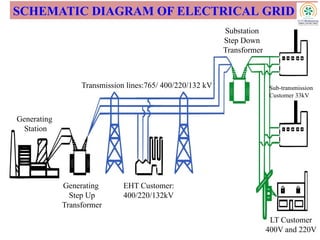
![INTRODUCTION
Classification and location of the fault is increased in application of a distribution line due to
the operation of deregulated environment and its tendency to compete in the power sector for
maximum availability of the power supply.
Protection engineers find challenges in certain applications like:-
Classification and Location of fault in a transmission and distribution line
Additional transients during fault which is not easily visible on inspection
Classification and location of fault in underground cable
repair requires large time and labour, cost is large, accuracy required is very high
To overcome the mentioned problems, following steps are taken:-
Necessary to develop an algorithm which can easily classify and locate the fault in a
transmission and distribution line. [1-3]
SECTION : I
6/93](https://image.slidesharecdn.com/mltrasmissionline-260106104221-1d49760c/85/Power-trasmission-line-energy-saving-through-Machine-Learning-6-320.jpg)


![LITERATURE REVIEW
Various techniques to estimate accurate fault location in a Transmission line
Impedance measurement based method
Single ended Impedance based method use line terminal voltage and current before and
during the fault
Test system (400 kV, 300 km)
Fault location error less than 1%.
The main drawback is that they have poor accuracy for high impedance fault.
SECTION : I
[Capar, A.; Arsoy, A. B. (2015) A performance oriented impedance based fault location
algorithm for series compensated transmission lines,” Electrical Power and Energy Systems 71
pp. 209–214 ]
10/93
For Transmission line](https://image.slidesharecdn.com/mltrasmissionline-260106104221-1d49760c/85/Power-trasmission-line-energy-saving-through-Machine-Learning-10-320.jpg)
![LITERATURE REVIEW
Two-ended impedance based technique is applied to localize the fault to eradicate the single
end impedance methods in the Transmission line.
The drawback of this technique is a high calculation burden due to measurement of current
and voltage signal at both ends of the TL.
However increase the accurateness to localize the fault
SECTION : I
[Dabbagh, M. A.; Kapuduwage, S. K. (2005) Using instantaneous values for estimating fault
locations on series compensated transmission lines, Electric Power Systems Research, vol. 76,
issues. 1-3 , pp. 25-32.]
11/93](https://image.slidesharecdn.com/mltrasmissionline-260106104221-1d49760c/85/Power-trasmission-line-energy-saving-through-Machine-Learning-11-320.jpg)
![LITERATURE REVIEW
Impedance based technique is applied to classify the fault to eradicate the single end
impedance methods in the Transmission line.
The Advantage of this method is its effectiveness in case of several typical cases
The drawback of this technique is failed particularly in case of high impedance faults and
also at other typical cases
SECTION : I
[Prasada, C. D.; Srinivasua, N. (2015) Fault Detection in Transmission Lines using Instantaneous
Power with ED based Fault Index, Procedia Technology , 21, pp. 132 – 138.]
12/93](https://image.slidesharecdn.com/mltrasmissionline-260106104221-1d49760c/85/Power-trasmission-line-energy-saving-through-Machine-Learning-12-320.jpg)
![LITERATURE REVIEW
SECTION : I
[Hasheminejad, S.; Seifossadat, S. G.; Joorabian, M. M. (2016) Traveling-wave-based protection of
parallel transmission lines using Teager energy operator and fuzzy systems, IET Gener. Transm.
Distrib., Vol. 10, Iss. 4, pp. 1067–1074]
13/93
Intelligent traveling-wave (TW) based method is applied in transmission line for the location and
classification of faults in parallel Transmission line.
To extracts the TWs from the power signal Teager energy operator (TEO) is implemented.
The time difference between the first two TWs and the TWs’ propagation speed is applied to
analyze the faults
The effect of Current transformer (CT) saturation is not considered in the algorithms
This technique has less error to localize the faults in high resistance faults path.
But the main drawbacks are
Calculation burden and Costly
High sampling frequency is used, which is a challenging task for real time use](https://image.slidesharecdn.com/mltrasmissionline-260106104221-1d49760c/85/Power-trasmission-line-energy-saving-through-Machine-Learning-13-320.jpg)
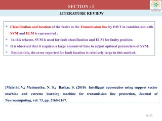
![LITERATURE SURVEY
Wavelet packet based technique for fault location in a series compensated transmission line .
Single ended measurement, half cycle of post fault voltage
Wavelet packet decomposition, Support vector machine are implemented
Feature extraction, energy, more features
Noise eliminated by low pass filter
Large value of fault resistance taken
Performance evaluation by absolute error and mean square error
Error reported is large
SECTION:I
[Yusuff, A. A.; Fei, C. A.; Jimoh A.; Munda, J. L. (2011) Fault location in a series compensated
transmission line based on wavelet packet decomposition and support vector regression, Electric
Power Systems Research, vol. 81, Issue 7, pp. 1258-1265.]
17/173](https://image.slidesharecdn.com/mltrasmissionline-260106104221-1d49760c/85/Power-trasmission-line-energy-saving-through-Machine-Learning-15-320.jpg)
![LITERATURE REVIEW
In order to select the best features for better performance, a feature selection algorithm is
proposed.
His algorithm involved a feature-weighted version of the k-nearest-neighbor which is able to
capture complex dependency of the target function on its input and makes use of the leave-
one-out error as a natural regularization.
The new algorithm for feature selection provided improvement in prediction quality and
presented a novel way of exploring neural data.
SECTION : I
[Amir Navot, Lavi shpigelman, Naftali tishby, Eilon vaadia, “Nearest neighbor based feature
selection for regression and its application to neural activity,” in Proc.2006. Advances in neural
information processing systems, Vol.18, pp. 995-1002.]
16/173](https://image.slidesharecdn.com/mltrasmissionline-260106104221-1d49760c/85/Power-trasmission-line-energy-saving-through-Machine-Learning-16-320.jpg)


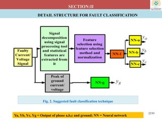


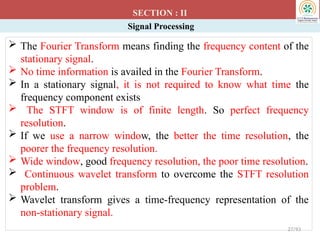


![ It is the process of choosing a small subset from all the features that is sufficient to predict the target properly.
It helps in reducing the computational complexity of learning and prediction algorithms and enhances the
prediction accuracy.[21]
SECTION:II
FEATURE SELECTION
36/93
Fig. 6. Feature selection algorithm](https://image.slidesharecdn.com/mltrasmissionline-260106104221-1d49760c/85/Power-trasmission-line-energy-saving-through-Machine-Learning-36-320.jpg)
![FEATURE SELECTION METHOD
SECTION:II
FORWARD FEATURE SELECTION (FFS) METHOD
Features are iteratively added into a growing subset of inputs and in each step, feature showing
the highest score is added and the rest is discarded.[22]
An evaluation function to assign scores to features.
Evaluation function used is
leave one out (LOO)
Mean square error (MSE) of the k-nearest-neighbor (KNN) estimator.[23]
KNN estimator is the weighted average of nearest neighbor.
Evaluation function is negative (halved) MSE of the weighted KNN estimator.
It helps to search a locally optimal weight vector by giving scores to weight vector over the
features.
Thereafter each feature is provided with a rank by the resulting weight which is applied further
to make a subset of optimal features.
Search algorithm to search for a subset with a high score
37/93](https://image.slidesharecdn.com/mltrasmissionline-260106104221-1d49760c/85/Power-trasmission-line-energy-saving-through-Machine-Learning-37-320.jpg)
![PARTICLE SWARM OPTIMIZATION BASED FEATURE SELECTION
SECTION:II
Stochastic optimization based technique [25]
Particle interacts among them to find global optimal solution
Each particle has its own Position and velocity
Position of each particle is given in binary form representing the energy feature.
Fitness function of each particle
Updated by pbest and gbest
Best solution achieved in every step of the iteration process so far
Best solution obtained so far by any particle in the population
Update new position and velocity
Choice of particle based on the fitness function of the new updated particle.
38/93](https://image.slidesharecdn.com/mltrasmissionline-260106104221-1d49760c/85/Power-trasmission-line-energy-saving-through-Machine-Learning-38-320.jpg)
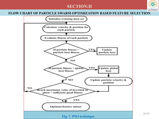
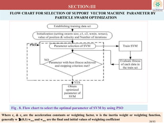
![GENETIC ALGORITHM BASED FEATURE SELECTION
SECTION:II
Stochastic search method , explores the search space to attain an optimal solution.
Operates with a set of population of chromosome represented by a string of
binary digits.
Selected chromosome for the next generation on the basis of a fitness function.
Each coefficient of DWT/WPT decomposition is represented by binary digit .
One of the feature is selected from the available six features for each coefficient.[27]
• Reproduction,
• Cross-over
• Mutation.
Reproduction :
Entire set of chromosomes gets a rank based on the fitness function and
The selection of chromosomes is done based on the highest ranking.
41/93](https://image.slidesharecdn.com/mltrasmissionline-260106104221-1d49760c/85/Power-trasmission-line-energy-saving-through-Machine-Learning-41-320.jpg)

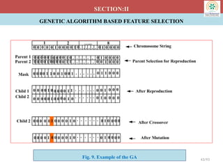
![ARTIFICIAL NEURAL NETWORK
Computational model, simulates structure & functional aspects of biological neural network
Multilayer feedforward neural network with gradient descent backpropagation training
algorithm[28]
SECTION:II
44/93
Fig. 10. ANN structure](https://image.slidesharecdn.com/mltrasmissionline-260106104221-1d49760c/85/Power-trasmission-line-energy-saving-through-Machine-Learning-44-320.jpg)


![ Adaptive computational learning algorithm based on statistical learning theory in which the
original input vectors are non-linearly mapped into a high dimensional feature space and the
optimal hyper plane is determined to maximize the generalization ability. Global & Unique
solution, Does not converge into local minima, Prone to Overfitting [32]
SECTION:II
47/93
SUPPORT VECTOR MACHINE (SVM)
Fig. 13. SVM Structure](https://image.slidesharecdn.com/mltrasmissionline-260106104221-1d49760c/85/Power-trasmission-line-energy-saving-through-Machine-Learning-47-320.jpg)
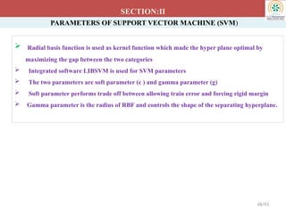
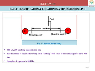
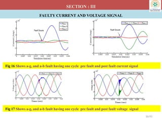
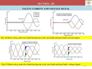
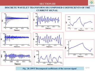
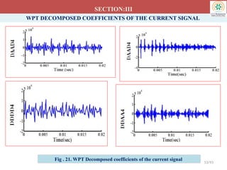
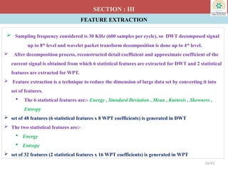
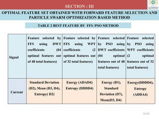
![OPTIMAL & NON-OPTIMAL FEATURE PLOT USING DWT
SECTION: III
Fig 22 (a) Optimal feature plot of
coefficient standard deviation
[D2] of energy of current signal
using FFS method
Fig .22 (b) Optimal feature plot of
coefficient standard deviation [D7]
of current signal using PSO method
56/93
Fig . 22(c). Non-optimal feature
plot of coefficient standard
deviation [D1] of current signal
Pattern of optimal feature is easy to predict whereas non-optimal feature gave unpredictable and erratic
pattern
So, concluded that optimal feature plot gives a distinct path for each value of fault distance whereas non-
optimal feature plot shows a random path which makes the prediction of fault classification and location
quite difficult.](https://image.slidesharecdn.com/mltrasmissionline-260106104221-1d49760c/85/Power-trasmission-line-energy-saving-through-Machine-Learning-56-320.jpg)
![OPTIMAL & NON-OPTIMAL FEATURE PLOT USING WPT
SECTION: III
Fig 23 (a) Optimal feature plot of
coefficient Energy [ADAD4] of
current signal by using FFS
Fig .23 (b) Optimal feature plot
of coefficient Energy[DDDD4]
of current signal by using PSO
57/93
Fig . 23(c). Non-optimal feature
plot of coefficient DDAA4
energy of current signal
Pattern of optimal feature is easy to predict whereas non-optimal feature gave unpredictable and erratic
pattern
So, concluded that optimal feature plot gives a distinct path for each value of fault distance whereas non-
optimal feature plot shows a random path which makes the prediction of fault classification and location
quite difficult.](https://image.slidesharecdn.com/mltrasmissionline-260106104221-1d49760c/85/Power-trasmission-line-energy-saving-through-Machine-Learning-57-320.jpg)
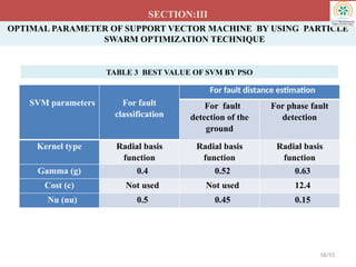
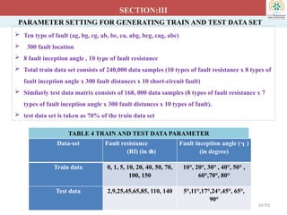
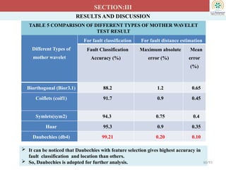
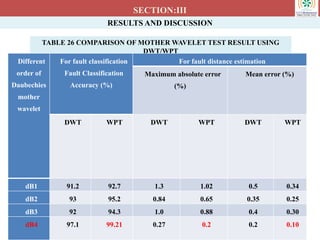
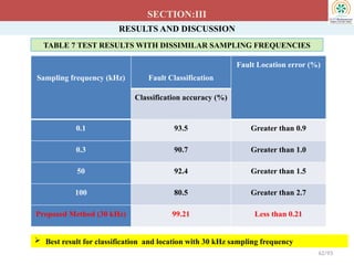
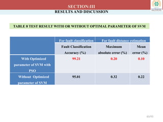

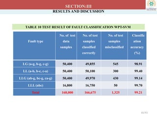
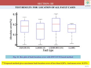
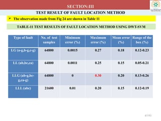
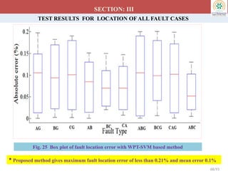
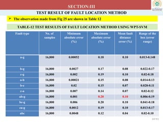
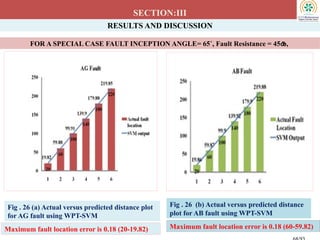
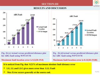

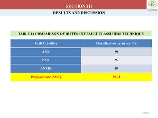
![RESULTS AND DISCUSSION
SECTION:III
TABLE 15 COMPARISON WITH OTHER RESEARCHER
74/93
Schemes
Fault Classification
Fault Location
error (%)
No. of test samples Classification
accuracy (%)
Method in [34] - - Greater than 0.30
Method in [35] 28,800 99.11 Greater than 0.45
Method in [36] 200 97.2 -
Method in [37] - - Greater than 0.90
Method in [38] - - Greater than 1.0
Method in [39] - - More than 2.0
Proposed Method
(WPT-SVM)
168,000 99.21 Less than 0.21](https://image.slidesharecdn.com/mltrasmissionline-260106104221-1d49760c/85/Power-trasmission-line-energy-saving-through-Machine-Learning-74-320.jpg)
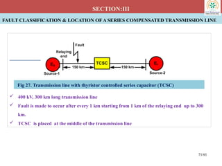

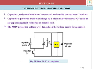
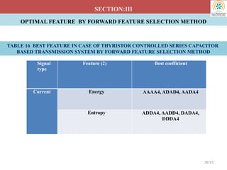


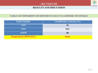
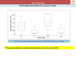
![RESULTS AND DISCUSSION
SECTION:III
TABLE 20 COMPARISON WITH OTHER RESEARCHER
83/93
Schemes
Fault Classification
Fault Location
error (%)
No. of test samples Classification accuracy
(%)
Method in [40] 25200 Average accuracy
93.92%
-
Method in [41] 200 More than 95.09% -
Method in [42] 25600 More than 97.2% -
Method in [43] - - Maximum error
5.28%
Method in [44] - - Maximum error
5%
Method in [45] - - Maximum error
3%
Proposed Method 168000 98.36% Less than 0.28](https://image.slidesharecdn.com/mltrasmissionline-260106104221-1d49760c/85/Power-trasmission-line-energy-saving-through-Machine-Learning-83-320.jpg)

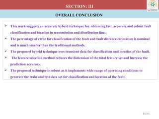

![APPENDICES
FOR TRANSMISSION LINE SYSTEM
PARAMETERS OF THE SYSTEM UNDER STUDY [20]
(i) Receiving and Sending end voltage source parameter : Positive sequence impedance (Z1): 1.31+ j16.0 Ω
Zero sequence impedance (Z0): 2.22 + j 27.6 Ω ; Frequency of the system: 50 Hz
(ii) Parameter of long transmission line :
Length: 300 km, Voltage: 400 kV; Impedance of positive sequence = 8.15 + j 94.5
Impedance of zero sequence = 92.5 + j 308 ; Positive sequence capacitance = 14 nF/km, Zero sequence
capacitance = 7.5 nF/km
DETAILS OF TCSC PARAMETER
L = 61.9 mH, C = 21.977 μ F
Details of the parameters of PSO based feature selection
C1= 2.05, C2= 2.05, Particle size = 60, No. of iteration = 100, Wmin= 0.4, Wmax= 0.9
Details of the parameters of ANN are given in Table 68 and optimal value of SVM parameter by PSO is given in Table
3
87/93](https://image.slidesharecdn.com/mltrasmissionline-260106104221-1d49760c/85/Power-trasmission-line-energy-saving-through-Machine-Learning-87-320.jpg)