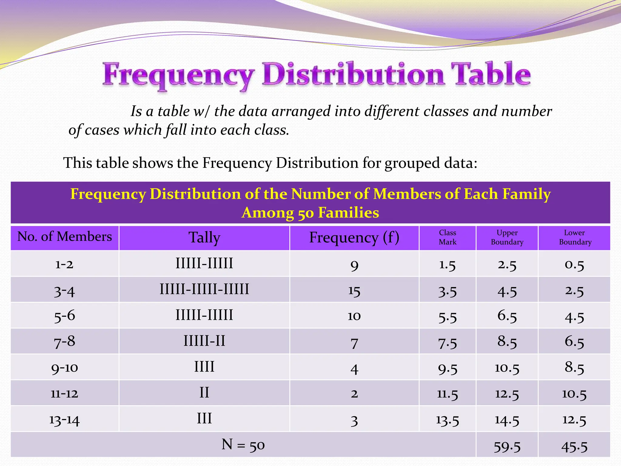
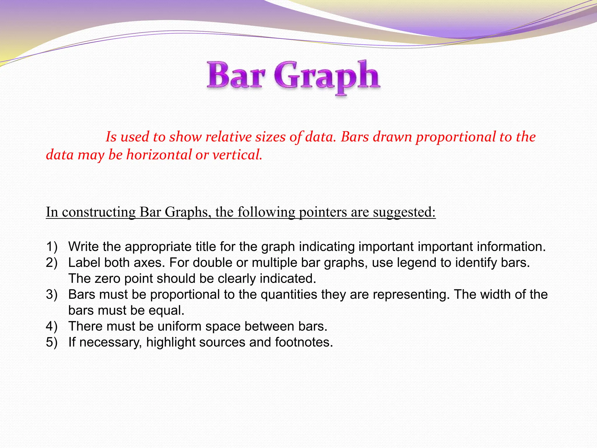
INTRODUCTION
In Statistics, we’ve studied about the Frequency
Distribution based on the given data. These data were
classified as grouped and ungrouped. Based on the data
given, we can determine how the table should be. For
making a Frequency Distribution Table for ungrouped
data is way too easy, while for grouped data, is quite
complicated.
The Frequency Distribution table is not only the
way to express or to file the data. We also use graphs to not
just illustrate the data given but also to be able us to
understand the data through in visual way. There are 5
different graphs: Bar Graph, Histogram, Frequency
Polygon, Pie Chart and the OGIVE Chart.
TABLE OF
CONTENTS
Title…………………………….…….Slide1
Introduction……………............…..Slide2
Table of Contents...………………..Slide3
Frequency Distribution…………...Slide 4
Bar Graph……………………….…..Slide 5-6
Histogram…………………………...Slide 7-8
Frequency Polygon…………….….Slide 9-10
Pie Chart…………………………….Slide 11-12
OGIVE Chart………………………..Slide 13-14
Generalization……………………...Slide 15
Credits……………………………….Slide 16
Is a table w/ the data arranged into different classes and number
of cases which fall into each class.
This table shows the Frequency Distribution for grouped data:
Frequency Distribution of the Number of Members of Each Family
Among 50 Families
No. of Members Tally Frequency (f) Class
Mark
Upper
Boundary
Lower
Boundary
1-2 IIIII-IIIII 9 1.5 2.5 0.5
3-4 IIIII-IIIII-IIIII 15 3.5 4.5 2.5
5-6 IIIII-IIIII 10 5.5 6.5 4.5
7-8 IIIII-II 7 7.5 8.5 6.5
9-10 IIII 4 9.5 10.5 8.5
11-12 II 2 11.5 12.5 10.5
13-14 III 3 13.5 14.5 12.5
N = 50 59.5 45.5
Is used to show relative sizes of data. Bars drawn proportional to the
data may be horizontal or vertical.
In constructing Bar Graphs, the following pointers are suggested:
1) Write the appropriate title for the graph indicating important important information.
2) Label both axes. For double or multiple bar graphs, use legend to identify bars.
The zero point should be clearly indicated.
3) Bars must be proportional to the quantities they are representing. The width of the
bars must be equal.
4) There must be uniform space between bars.
5) If necessary, highlight sources and footnotes.
0
2
4
6
8
10
12
14
16
1 to 2 3 to 4 5 to 6 7 to 8 9 to 10 11 to 12 13 to 14
Bar Graph of Frequency Distribution of the No. of
Members of each Family Among 50 Families
Frequency Distribution
of the No. of Members of
each Family Among 50
Students
Figure 2.1 Bar Graph
It is a graph that is like the bar graph but
only differ in the bars which is joined together and
instead of using class intervals it uses the class
boundaries (LB – UB).
It consists of adjacent rectangles whose
width is the distance from the lower to the upper
class boundary and the height is the corresponding
frequency.
0
2
4
6
8
10
12
14
16
Histogram of the Frequency Distribution of the
No. of Members of Each Family Among 50
Families
0.5 2.5 4.5 6.5 8.5 10.5 12.5 14.5
Figure 2.2 Histogram
It shows the relationship between two or more sets of
continuous data. For instance, it may show the relationship
between a population and time, or liquid capacity and distance.
In Constructing Frequency Polygon, the following Pointers are suggested:
1) State clearly the title of the graph indicating important information about the data.
2) Label both axes. For multiple Frequency polygon, a legend will facilitate understanding
of the information the graph wants to convey. The zero point should be clearly
indicated.
3) Connect plotted points from left to right.
4) Sources and footnotes should be provided, if necessary.
5) For multiple Frequency Polygons, one line should be distinguished from the other. This
can be done through the use of color or line forms.
0
2
4
6
8
10
12
14
16
1 to 2 3 to 4 5 to 6 7 to 8 9 to 10 11 to 12 13 to 14
Frequency Polygon of Frequency Distribution of the
No. of Members of each Family Among 50 Families
Frequency Polygon of
Frequency
Distribution of the
No. of Members of
each Family Among
50 Families
Figure 2.3 Frequency Polygon
Is best used to compare parts to a whole.
The size of each sector of the circle is proportional
to the size of the category that it represents
To make a Circle Graph, the following pointers are suggested:
1) Organize the data on the table by providing column to the fractional parts
or percent each quantity is of the whole and the number of degrees
representing each fractional part.
2) On a circle, construct successive central angles using the number of
degrees representing each part.
3) Label each part with the appropriate title for the graph.
18%
30%
20%
14%
8%
6% 4%
Pie Chart of the Frequency Distribution of the No. of
Members of each Family Among 50 Families
1 to 2
3 to 4
5 to 6
7 to 8
9 to 10
11 to 12
13 to 14
Figure 2.4 Pie Chart
Is a Frequency polygon where the cumulative frequency of
each class is plotted against the corresponding class boundary.
For the same data, the less than ogive and the greater than
ogive are graphed in one grid. Take note of the importance of the
intersection of the ogives.
0
10
20
30
40
50
60
Less than Cumulative
Frequency
Greater than
Cumulative
Frequency
0.5 2.5 4.5 6.5 8.5 10.5 12.5 14.5
OGIVE Chart
Figure 2.5 OGIVE Chart
GENERALIZATIO
N
There are 4 Graphs to show the Frequency Distribution of
data. It is: Bar Graph, Histogram, Frequency Polygon and the
Pie Chart.
OGIVE Chart is used to illustrate the Less than cumulative
Frequency and the Greater than cumulative Frequency.
JOHN ROME R. ARANAS
Creator
SOURCES AND RESOURCES
Myself
New Century Mathematics by Phoenix
Publishing
Statistics: Rudiments and Analysis of Data
by ICS Publishing
Math Notebook
Ms. Charmaigne Marie Mahamis
Google
Wikipedia

Different Types of Graphs in Statistics.pptx

  • 2.
    INTRODUCTION In Statistics, we’vestudied about the Frequency Distribution based on the given data. These data were classified as grouped and ungrouped. Based on the data given, we can determine how the table should be. For making a Frequency Distribution Table for ungrouped data is way too easy, while for grouped data, is quite complicated. The Frequency Distribution table is not only the way to express or to file the data. We also use graphs to not just illustrate the data given but also to be able us to understand the data through in visual way. There are 5 different graphs: Bar Graph, Histogram, Frequency Polygon, Pie Chart and the OGIVE Chart.
  • 3.
    TABLE OF CONTENTS Title…………………………….…….Slide1 Introduction……………............…..Slide2 Table ofContents...………………..Slide3 Frequency Distribution…………...Slide 4 Bar Graph……………………….…..Slide 5-6 Histogram…………………………...Slide 7-8 Frequency Polygon…………….….Slide 9-10 Pie Chart…………………………….Slide 11-12 OGIVE Chart………………………..Slide 13-14 Generalization……………………...Slide 15 Credits……………………………….Slide 16
  • 4.
    Is a tablew/ the data arranged into different classes and number of cases which fall into each class. This table shows the Frequency Distribution for grouped data: Frequency Distribution of the Number of Members of Each Family Among 50 Families No. of Members Tally Frequency (f) Class Mark Upper Boundary Lower Boundary 1-2 IIIII-IIIII 9 1.5 2.5 0.5 3-4 IIIII-IIIII-IIIII 15 3.5 4.5 2.5 5-6 IIIII-IIIII 10 5.5 6.5 4.5 7-8 IIIII-II 7 7.5 8.5 6.5 9-10 IIII 4 9.5 10.5 8.5 11-12 II 2 11.5 12.5 10.5 13-14 III 3 13.5 14.5 12.5 N = 50 59.5 45.5
  • 5.
    Is used toshow relative sizes of data. Bars drawn proportional to the data may be horizontal or vertical. In constructing Bar Graphs, the following pointers are suggested: 1) Write the appropriate title for the graph indicating important important information. 2) Label both axes. For double or multiple bar graphs, use legend to identify bars. The zero point should be clearly indicated. 3) Bars must be proportional to the quantities they are representing. The width of the bars must be equal. 4) There must be uniform space between bars. 5) If necessary, highlight sources and footnotes.
  • 6.
    0 2 4 6 8 10 12 14 16 1 to 23 to 4 5 to 6 7 to 8 9 to 10 11 to 12 13 to 14 Bar Graph of Frequency Distribution of the No. of Members of each Family Among 50 Families Frequency Distribution of the No. of Members of each Family Among 50 Students Figure 2.1 Bar Graph
  • 7.
    It is agraph that is like the bar graph but only differ in the bars which is joined together and instead of using class intervals it uses the class boundaries (LB – UB). It consists of adjacent rectangles whose width is the distance from the lower to the upper class boundary and the height is the corresponding frequency.
  • 8.
    0 2 4 6 8 10 12 14 16 Histogram of theFrequency Distribution of the No. of Members of Each Family Among 50 Families 0.5 2.5 4.5 6.5 8.5 10.5 12.5 14.5 Figure 2.2 Histogram
  • 9.
    It shows therelationship between two or more sets of continuous data. For instance, it may show the relationship between a population and time, or liquid capacity and distance. In Constructing Frequency Polygon, the following Pointers are suggested: 1) State clearly the title of the graph indicating important information about the data. 2) Label both axes. For multiple Frequency polygon, a legend will facilitate understanding of the information the graph wants to convey. The zero point should be clearly indicated. 3) Connect plotted points from left to right. 4) Sources and footnotes should be provided, if necessary. 5) For multiple Frequency Polygons, one line should be distinguished from the other. This can be done through the use of color or line forms.
  • 10.
    0 2 4 6 8 10 12 14 16 1 to 23 to 4 5 to 6 7 to 8 9 to 10 11 to 12 13 to 14 Frequency Polygon of Frequency Distribution of the No. of Members of each Family Among 50 Families Frequency Polygon of Frequency Distribution of the No. of Members of each Family Among 50 Families Figure 2.3 Frequency Polygon
  • 11.
    Is best usedto compare parts to a whole. The size of each sector of the circle is proportional to the size of the category that it represents To make a Circle Graph, the following pointers are suggested: 1) Organize the data on the table by providing column to the fractional parts or percent each quantity is of the whole and the number of degrees representing each fractional part. 2) On a circle, construct successive central angles using the number of degrees representing each part. 3) Label each part with the appropriate title for the graph.
  • 12.
    18% 30% 20% 14% 8% 6% 4% Pie Chartof the Frequency Distribution of the No. of Members of each Family Among 50 Families 1 to 2 3 to 4 5 to 6 7 to 8 9 to 10 11 to 12 13 to 14 Figure 2.4 Pie Chart
  • 13.
    Is a Frequencypolygon where the cumulative frequency of each class is plotted against the corresponding class boundary. For the same data, the less than ogive and the greater than ogive are graphed in one grid. Take note of the importance of the intersection of the ogives.
  • 14.
    0 10 20 30 40 50 60 Less than Cumulative Frequency Greaterthan Cumulative Frequency 0.5 2.5 4.5 6.5 8.5 10.5 12.5 14.5 OGIVE Chart Figure 2.5 OGIVE Chart
  • 15.
    GENERALIZATIO N There are 4Graphs to show the Frequency Distribution of data. It is: Bar Graph, Histogram, Frequency Polygon and the Pie Chart. OGIVE Chart is used to illustrate the Less than cumulative Frequency and the Greater than cumulative Frequency.
  • 16.
    JOHN ROME R.ARANAS Creator SOURCES AND RESOURCES Myself New Century Mathematics by Phoenix Publishing Statistics: Rudiments and Analysis of Data by ICS Publishing Math Notebook Ms. Charmaigne Marie Mahamis Google Wikipedia