Download to read offline
![References
ArcGIS Resource Center. (2011). Slope (Spatial Analyst). Retrieved April, 2014, from http://help.arcgis.com/
en/arcgisdesktop/10.0/help/index.html#//009z000000v2000000.htm
Burrough, P. A., & McDonnel, R. A. (1998). Principles of Geographical Information Systems. Oxford University Press,
New York.
Malczewski, J. (n.d.). A new procedure for gridding elevation and stream line data with automatic removal of
spurious pits. International Journal of Geographical Information Science, 20.
NVE. (n.d.). Jordskred og flomskred. Retrieved April, 2014, from http://varsom.no/Global/Faktaark/Fakta
%205-13%20Jord%20og%20flom.pdf
Saaty, T. L. (2008). Decision making with the analytic hierarchy process [Journal Article]. Int. J. Services Sci-
ences, 1, 83-98. Retrieved from http://citeseerx.ist.psu.edu/viewdoc/download?doi=10.1.1
.409.3124&rep=rep1&type=pdf
GEG2230 • Exercise 5 page 12 of 12](https://image.slidesharecdn.com/21af6165-a1de-44ba-bc33-9bfc368bcfcb-150716121259-lva1-app6892/85/DidrikLilja-Assignment2-Report-13-320.jpg)

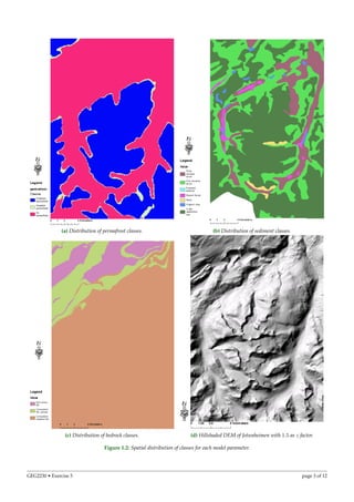
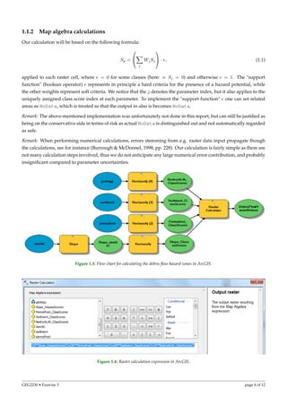
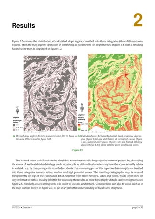
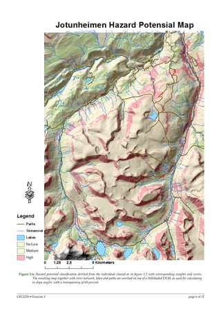
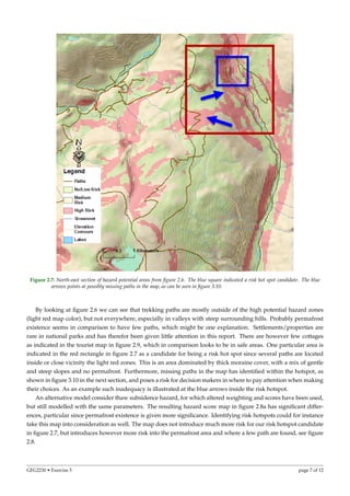
The document summarizes a multi-criteria analysis performed to identify hazard risk zones in Jotunheimen, Norway. Spatial data on slope, permafrost, sediment, and bedrock were analyzed using GIS and weighted aggregation. Hazard potential maps were produced and risk hotspots identified, including an area with paths located in high risk zones. The analysis could help prioritize preemptive measures, rescue resource allocation, and issuing of hazard warnings.