Download to read offline


![vi
LIST OF FIGURES
Figure Page
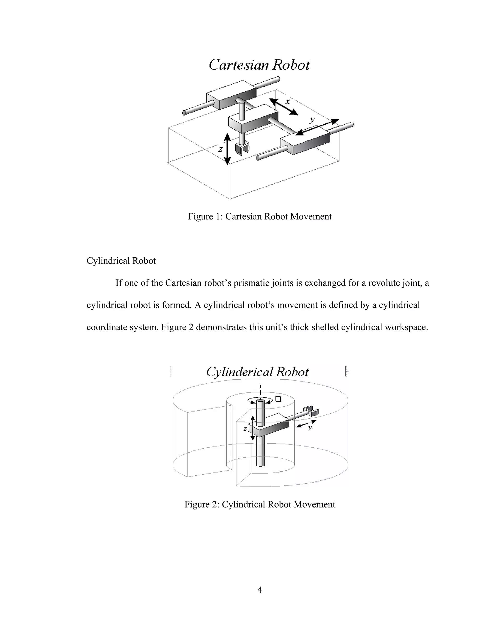
1: Cartesian Robot Movement ............................................................................................ 4
2: Cylindrical Robot Movement ......................................................................................... 4
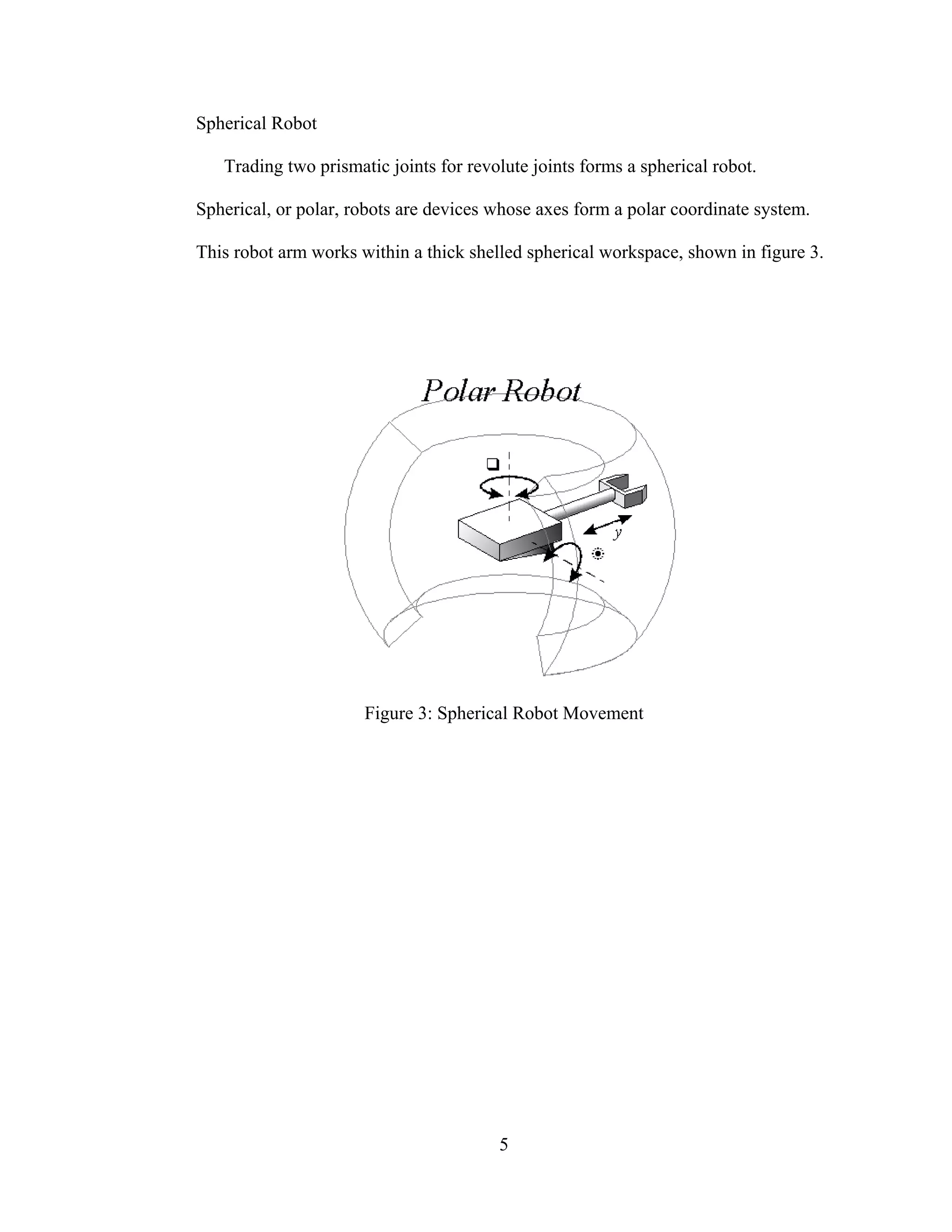
3: Spherical Robot Movement ............................................................................................ 5
4: Articulated Robot Motion [2] ......................................................................................... 6
5: Robot Comparison Chart [4]........................................................................................... 7
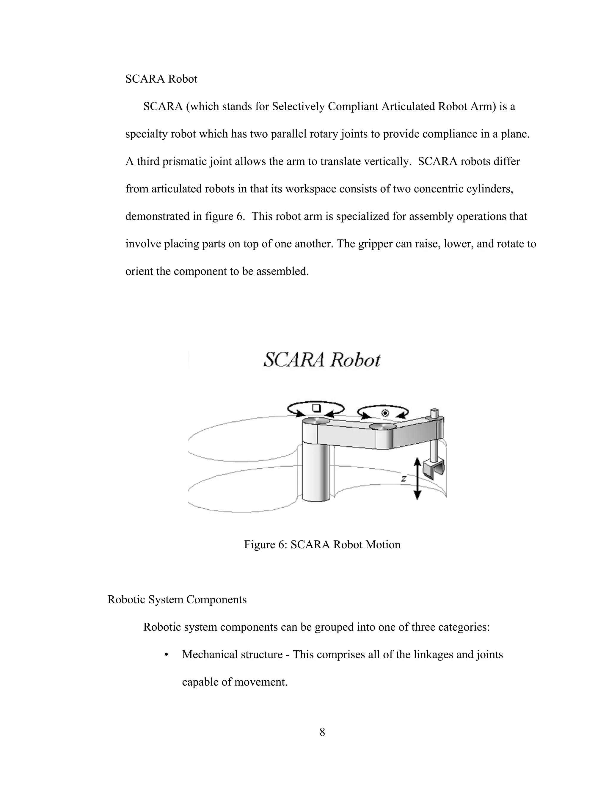
6: SCARA Robot Motion.................................................................................................... 8
7: Permanent Magnet Motor[1] ........................................................................................ 12
8: Variable Reluctance Motor[1] ...................................................................................... 13
9: Hybrid Stepper Motor[1] .............................................................................................. 14
10: Unifilar Motor Winding [1]........................................................................................ 15
11: Bifilar Motor Windings. Left: 6 Lead Motor. Right: 8 Lead Motor [1]..................... 16
12: Torque Degradation with Step Division [2] ............................................................... 19
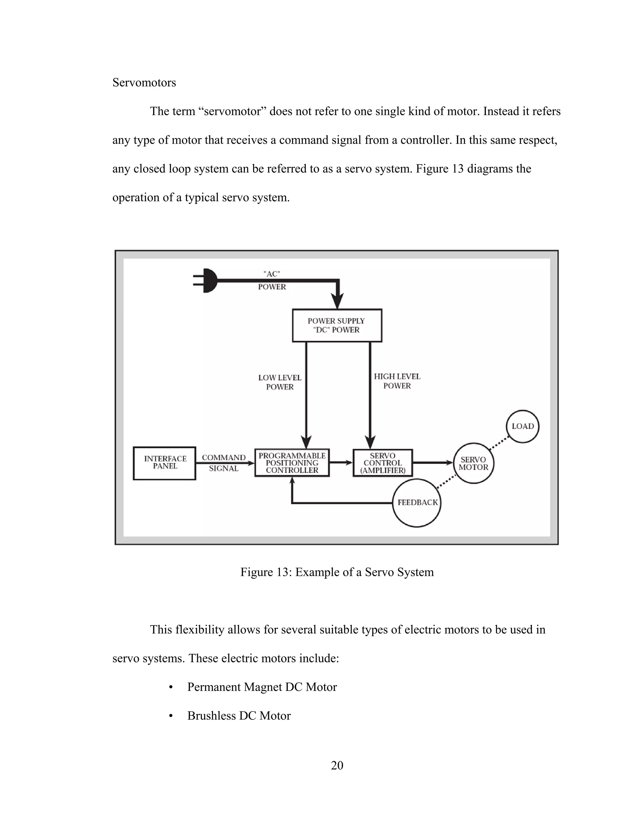
13: Example of a Servo System........................................................................................ 20
14: Permanent Magnet DC Motor..................................................................................... 22
15: Brushless DC Motor ................................................................................................... 23
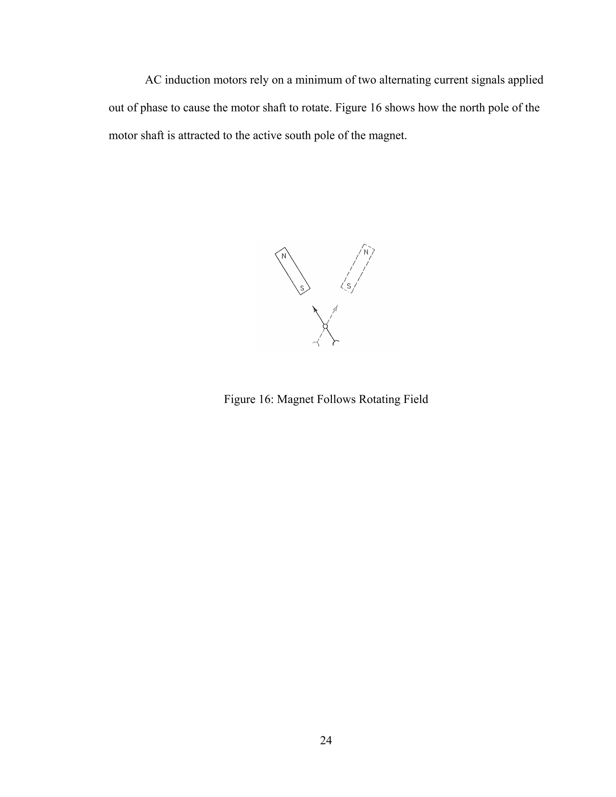
16: Magnet Follows Rotating Field .................................................................................. 24
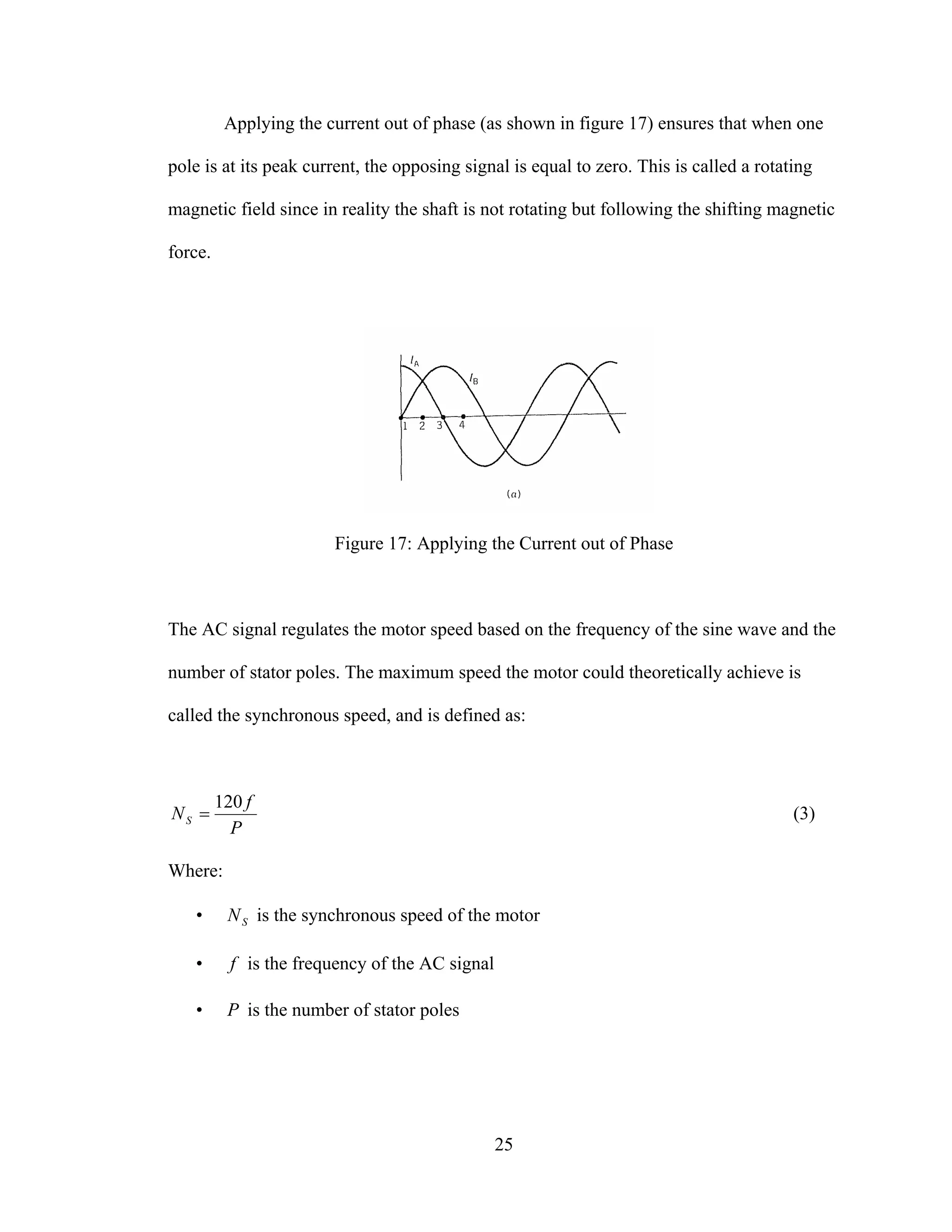
17: Applying the Current out of Phase ............................................................................. 25
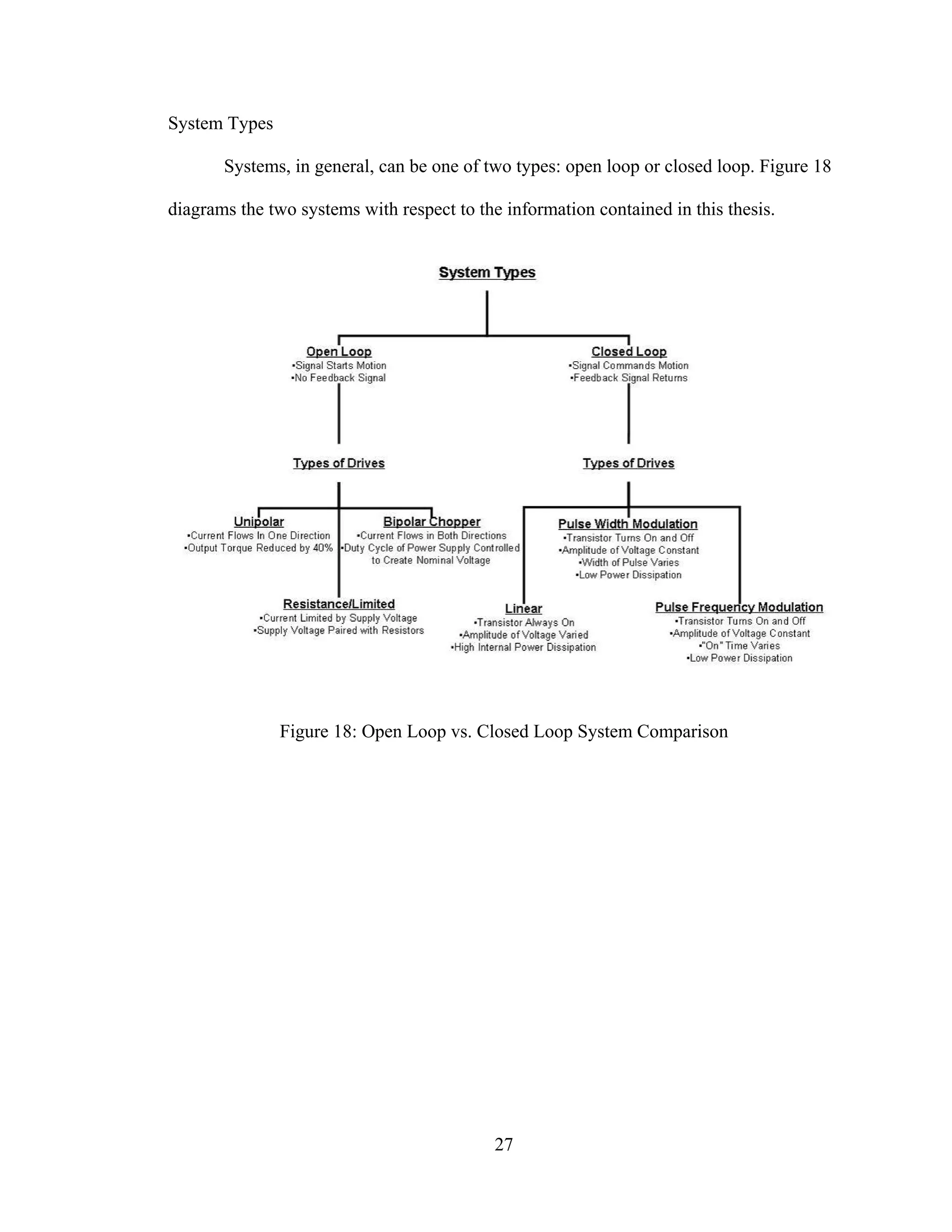
18: Open Loop vs. Closed Loop System Comparison...................................................... 27](https://image.slidesharecdn.com/designcontrolandimplementationofathreelink-190121102715/75/Design-control-and-implementation-of-a-three-link-6-2048.jpg)
![vii
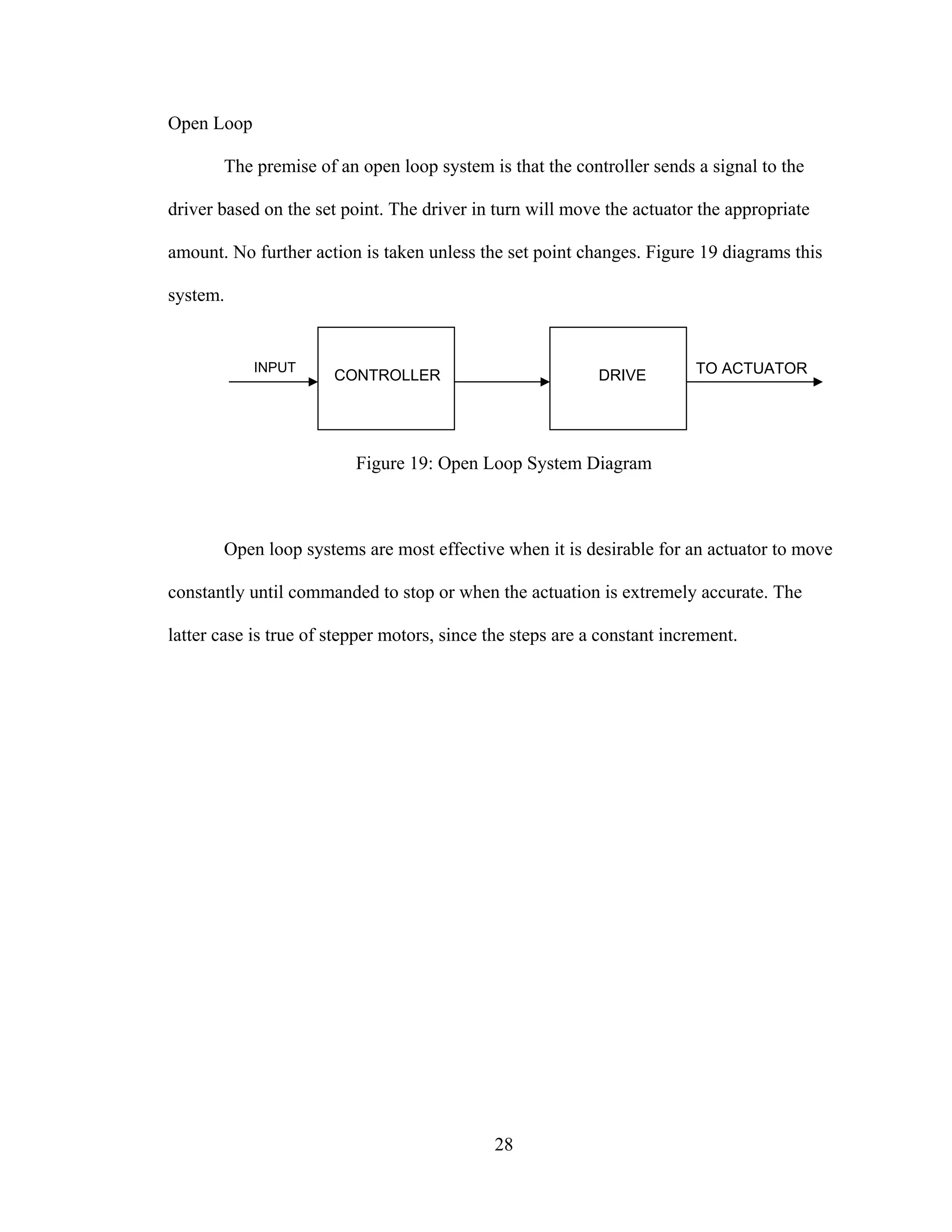
19: Open Loop System Diagram....................................................................................... 28
20: Closed Loop System................................................................................................... 29
21: Information Flow Between Driver and Motor[1] ....................................................... 30
22: Current Flow Through Unipolar Drive[5] .................................................................. 31
23: R/L Driver Circuit [5]................................................................................................. 32
24: H-bridge [5] ................................................................................................................ 33
25: Chopper Pulse Chart [5] ............................................................................................. 35
26: Bipolar Chopper Schematic [5] .................................................................................. 36
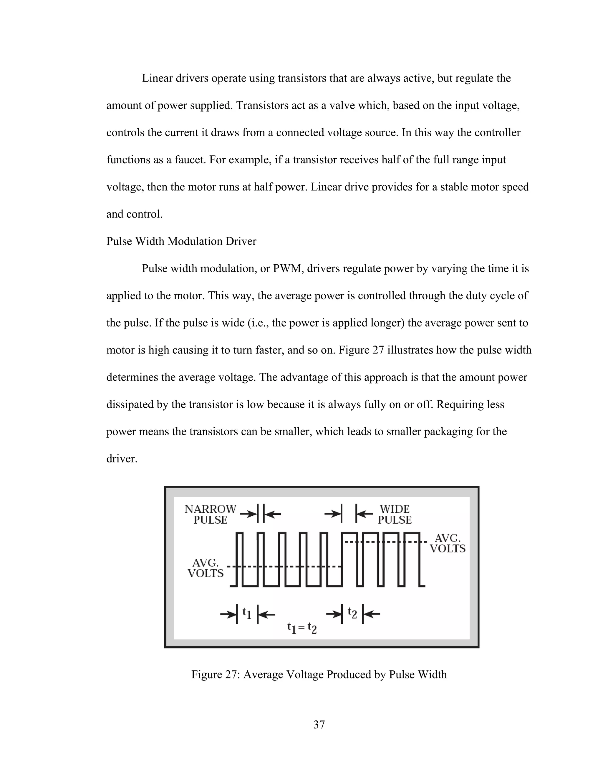
27: Average Voltage Produced by Pulse Width ............................................................... 37
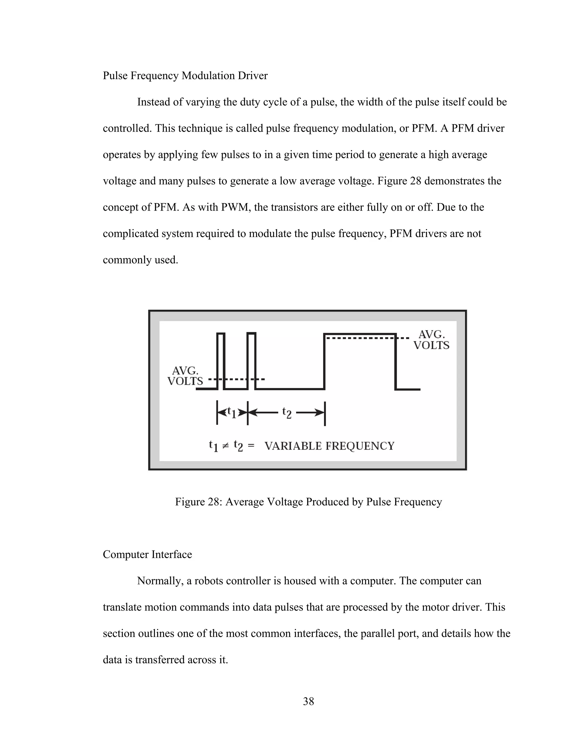
28: Average Voltage Produced by Pulse Frequency......................................................... 38
29: Layout of DB25 Parallel Port[1]................................................................................. 39
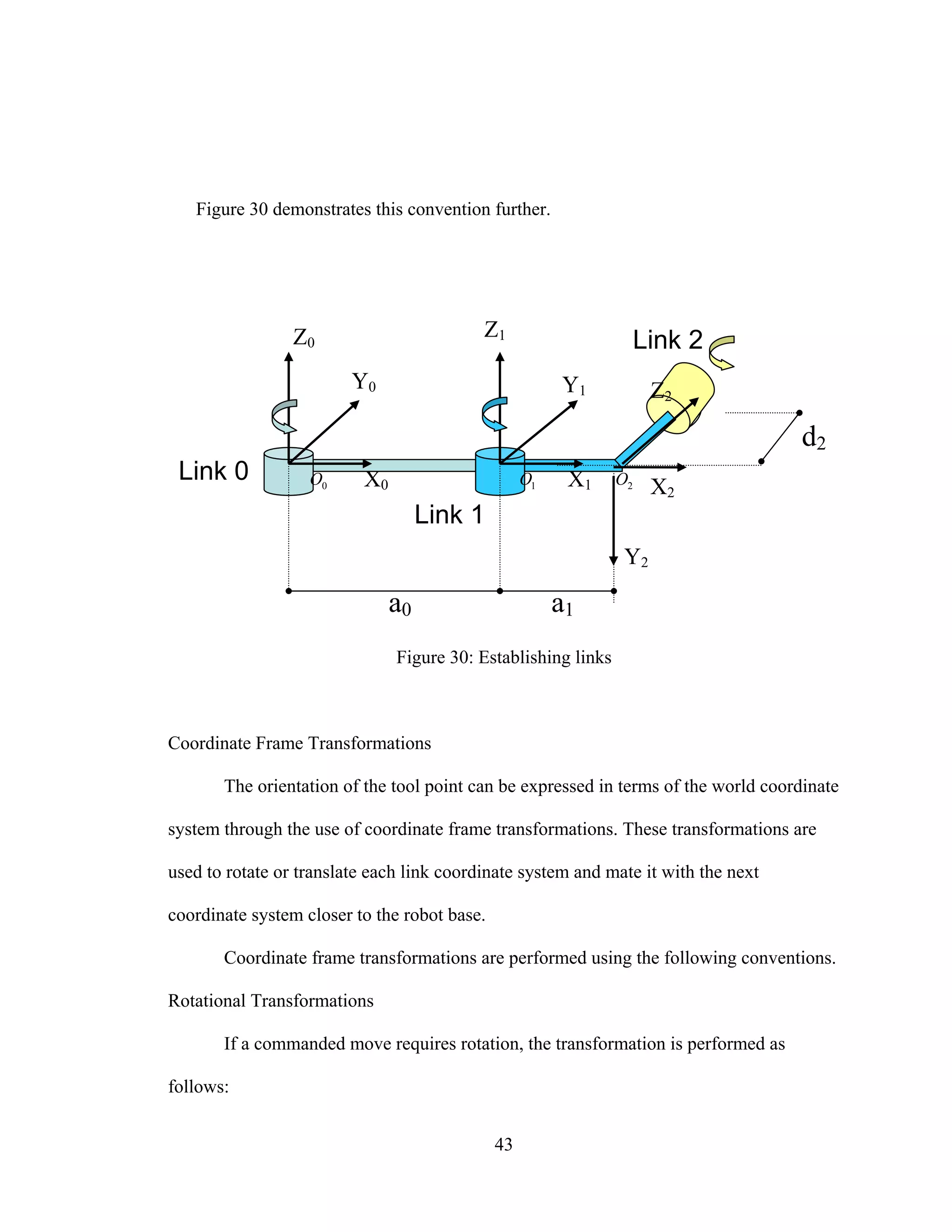
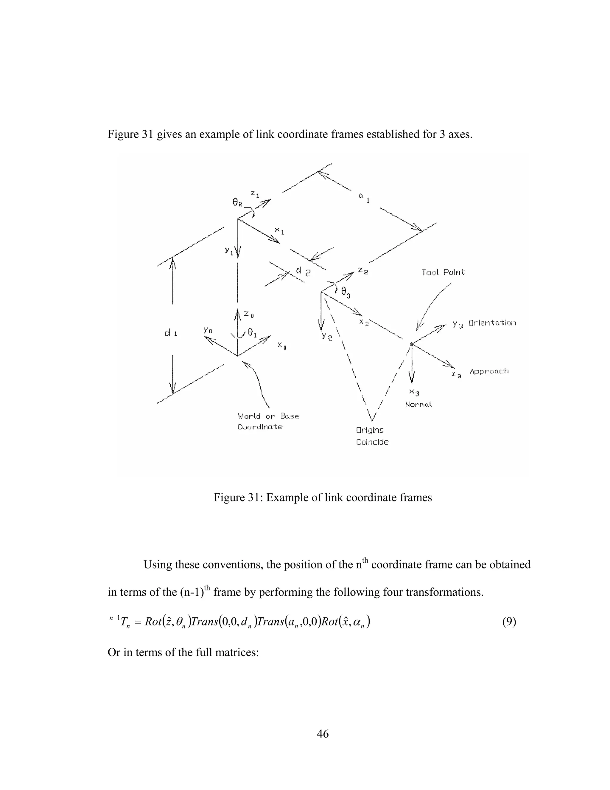
30: Establishing links........................................................................................................ 43
31: Example of link coordinate frames............................................................................. 46
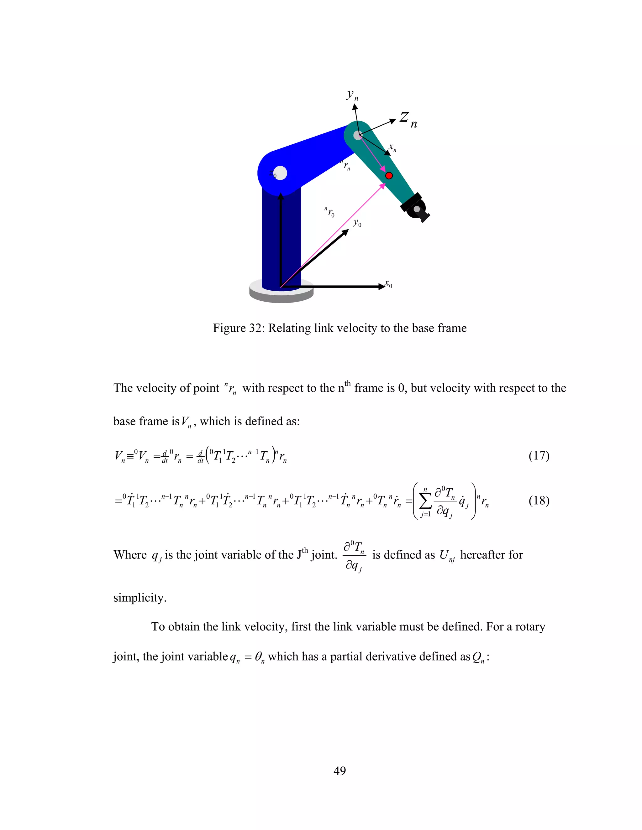
32: Relating link velocity to the base frame ..................................................................... 49
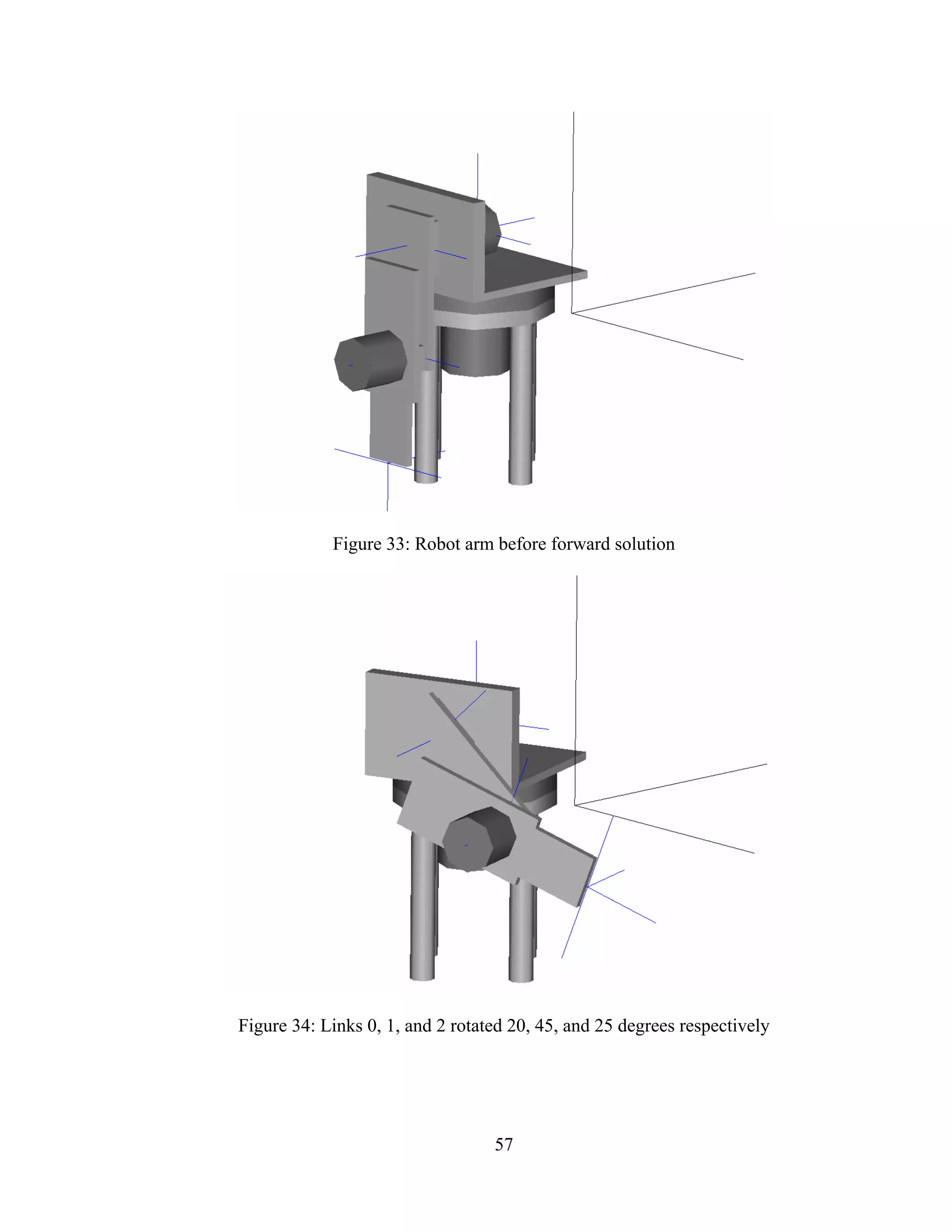
33: Robot arm before forward solution............................................................................. 57
34: Links 0, 1, and 2 rotated 20, 45, and 25 degrees respectively.................................... 57
35: Robot arm before inverse solution.............................................................................. 58
36: Robot arm translated to end point............................................................................... 59
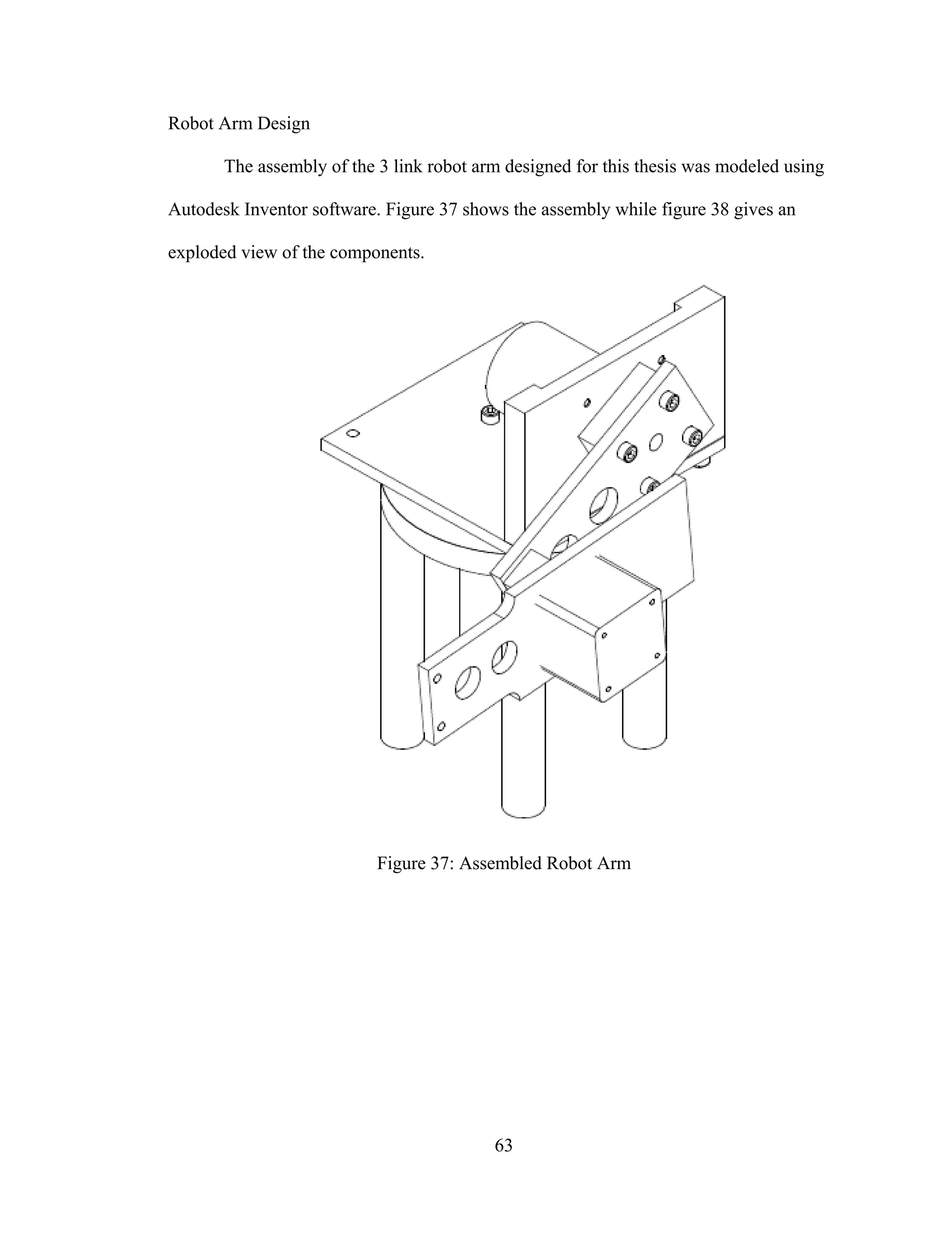
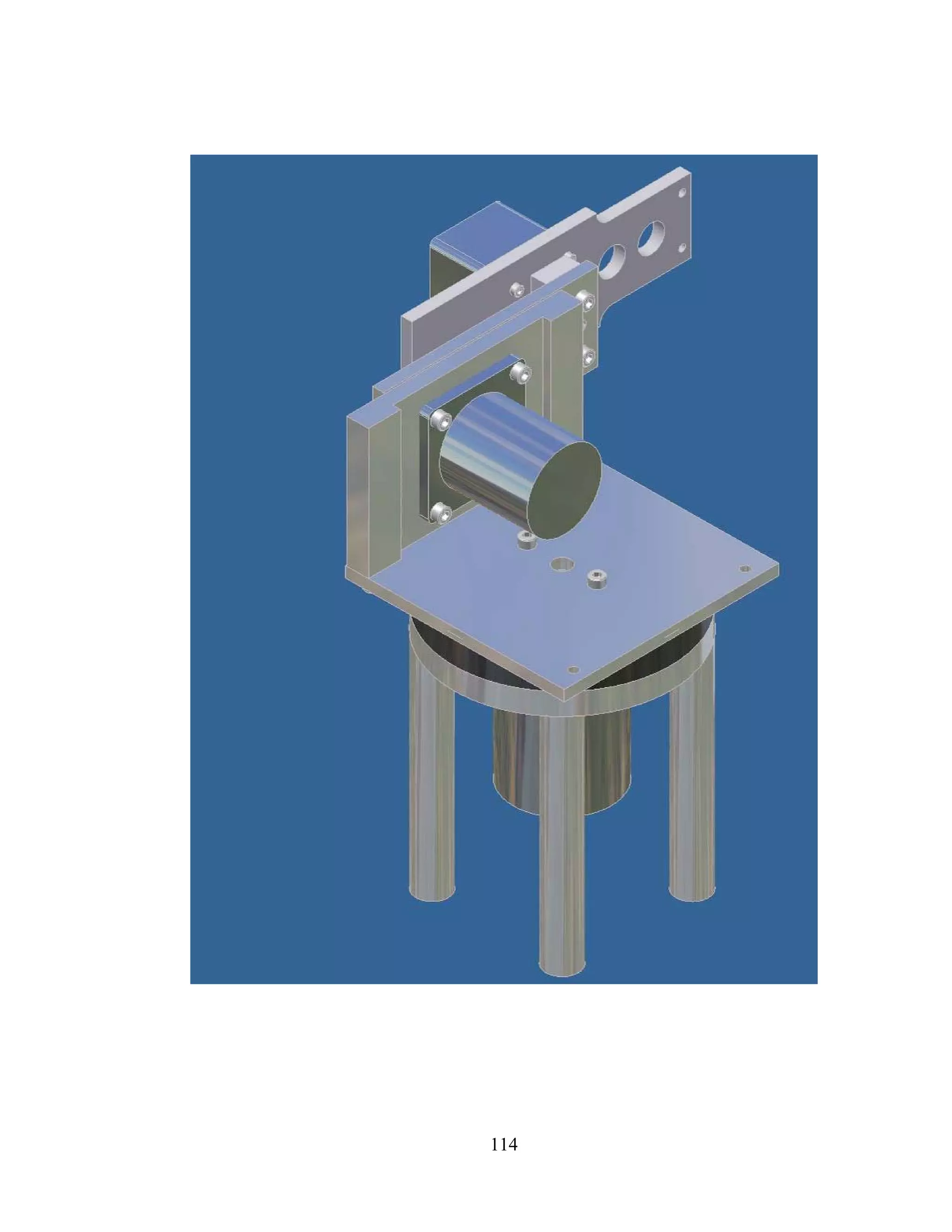
37: Assembled Robot Arm ............................................................................................... 63
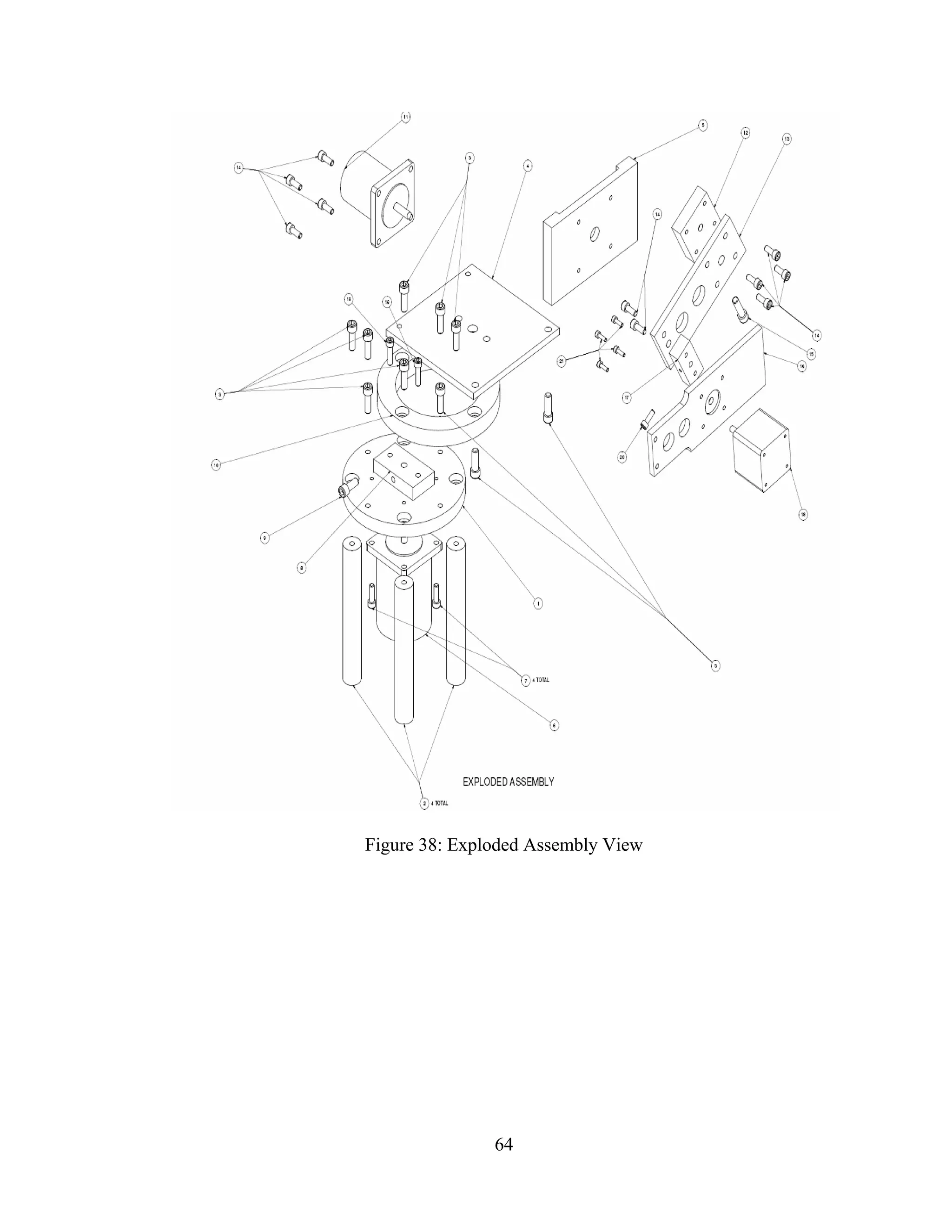
38: Exploded Assembly View .......................................................................................... 64
39: Robot Arm Reach Dimensions ................................................................................... 66
40: Link 0 Rotation........................................................................................................... 67
41: Rotation Range for Link 1 (a) and Link 2 (b)............................................................. 67](https://image.slidesharecdn.com/designcontrolandimplementationofathreelink-190121102715/75/Design-control-and-implementation-of-a-three-link-7-2048.jpg)
![viii
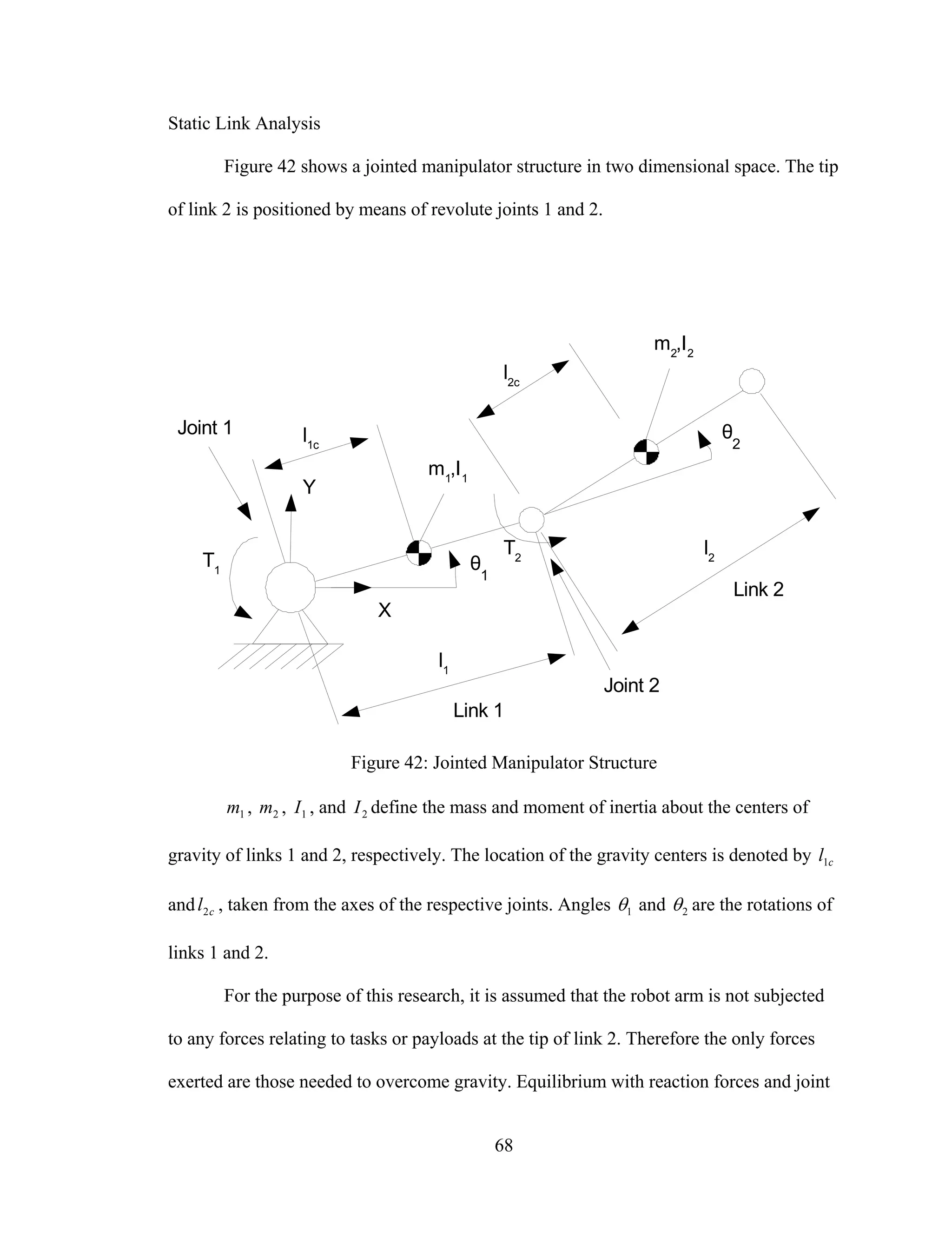
42: Jointed Manipulator Structure .................................................................................... 68
43: Forces and Moments Imposed on Manipulator Structure........................................... 69
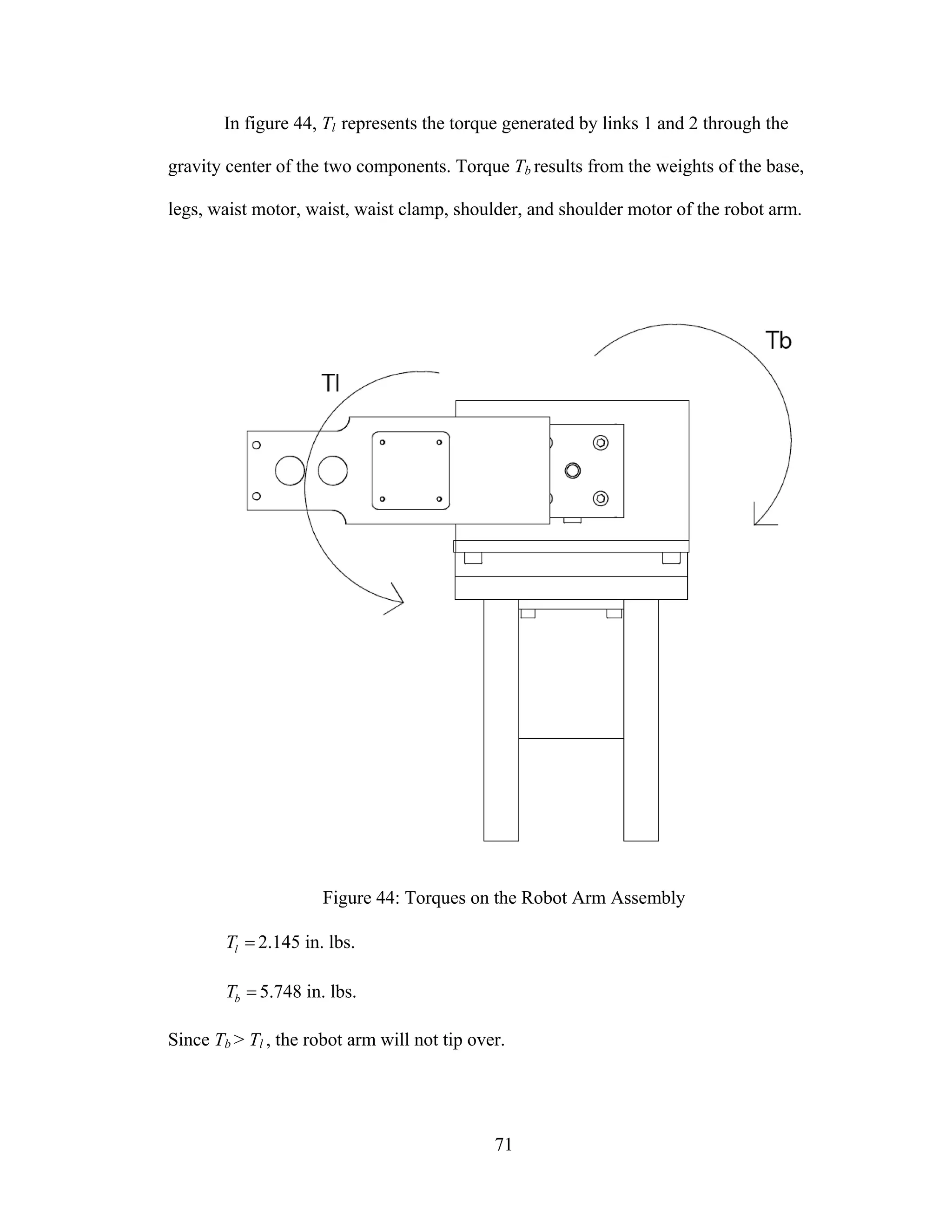
44: Torques on the Robot Arm Assembly ........................................................................ 71
45: Design Variables Link 2 ............................................................................................. 80
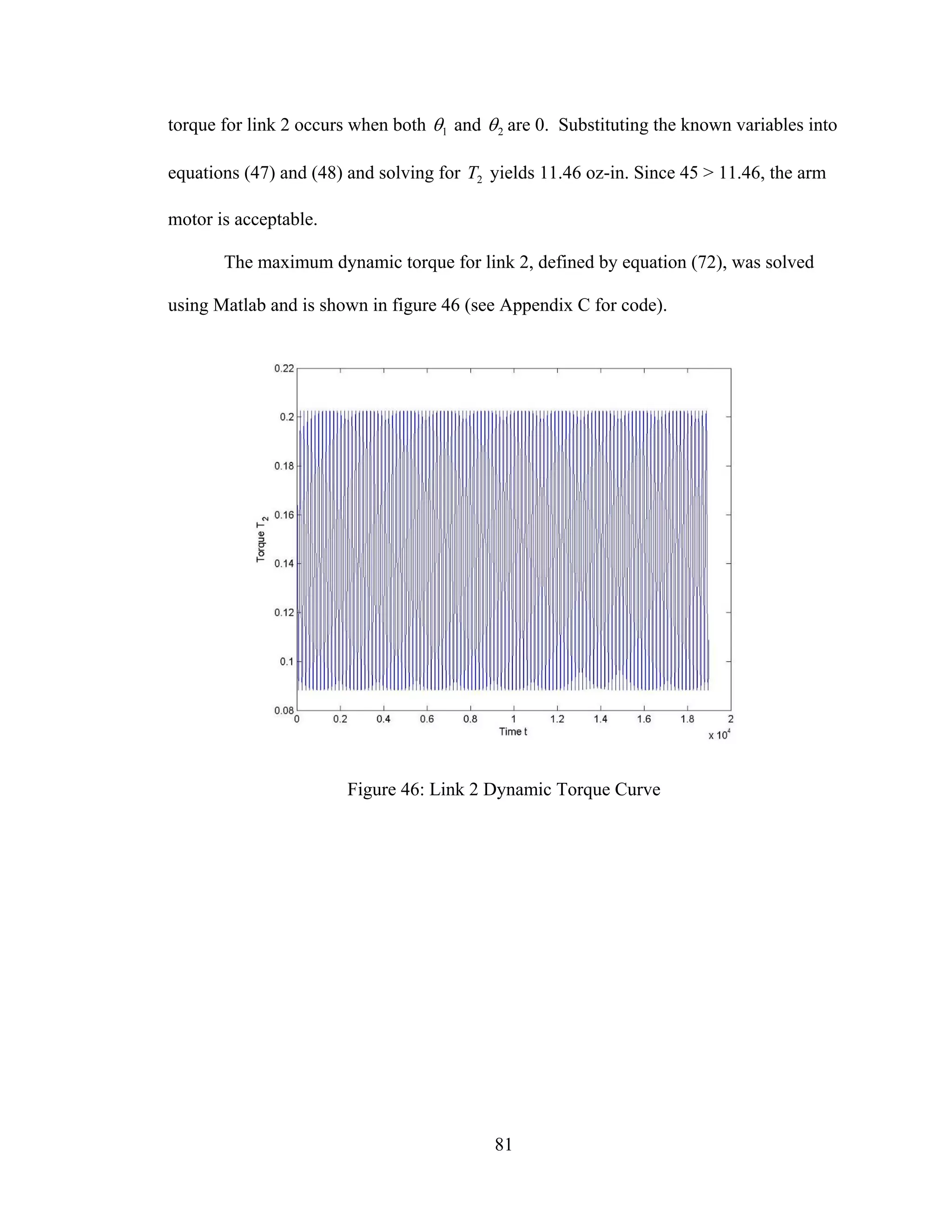
46: Link 2 Dynamic Torque Curve................................................................................... 81
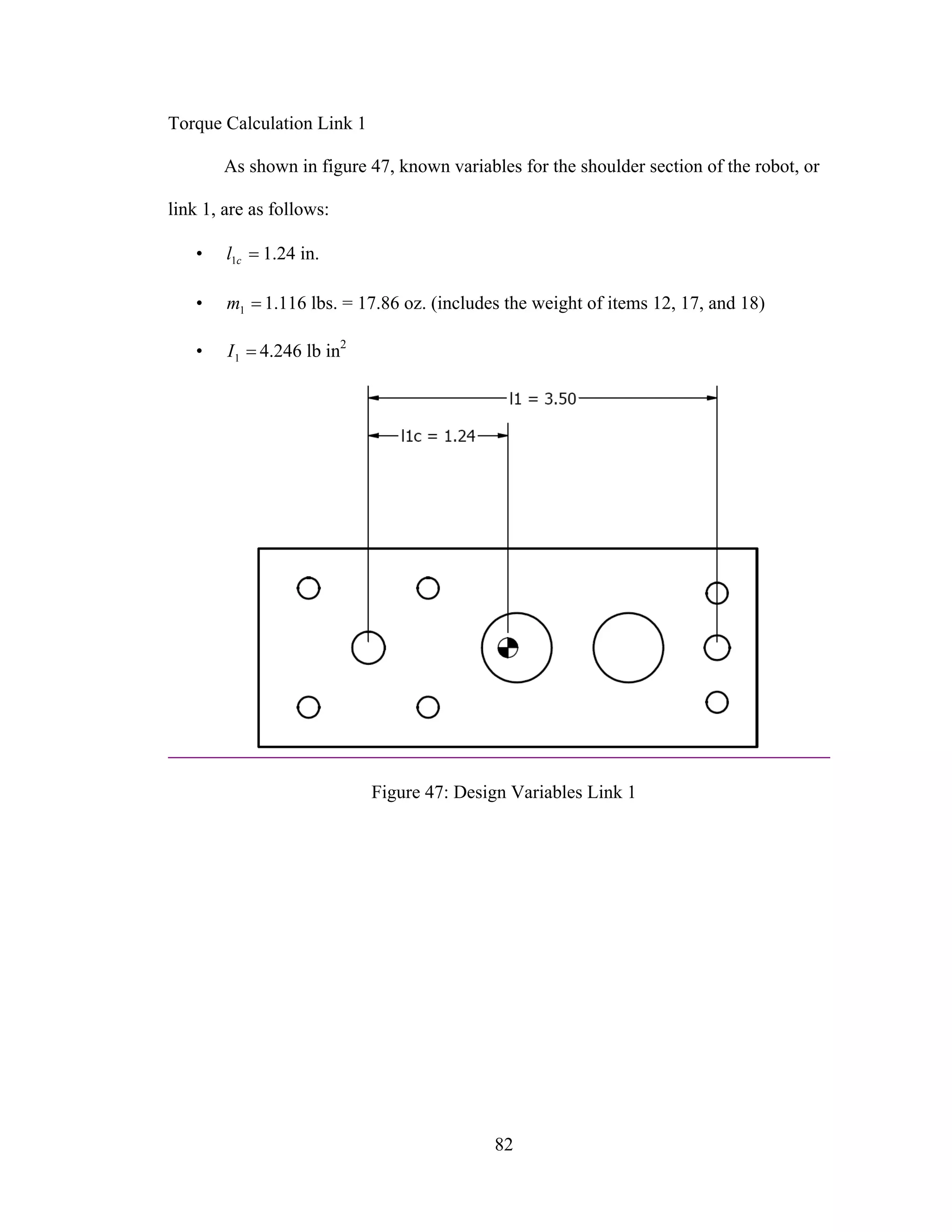
47: Design Variables Link 1 ............................................................................................. 82
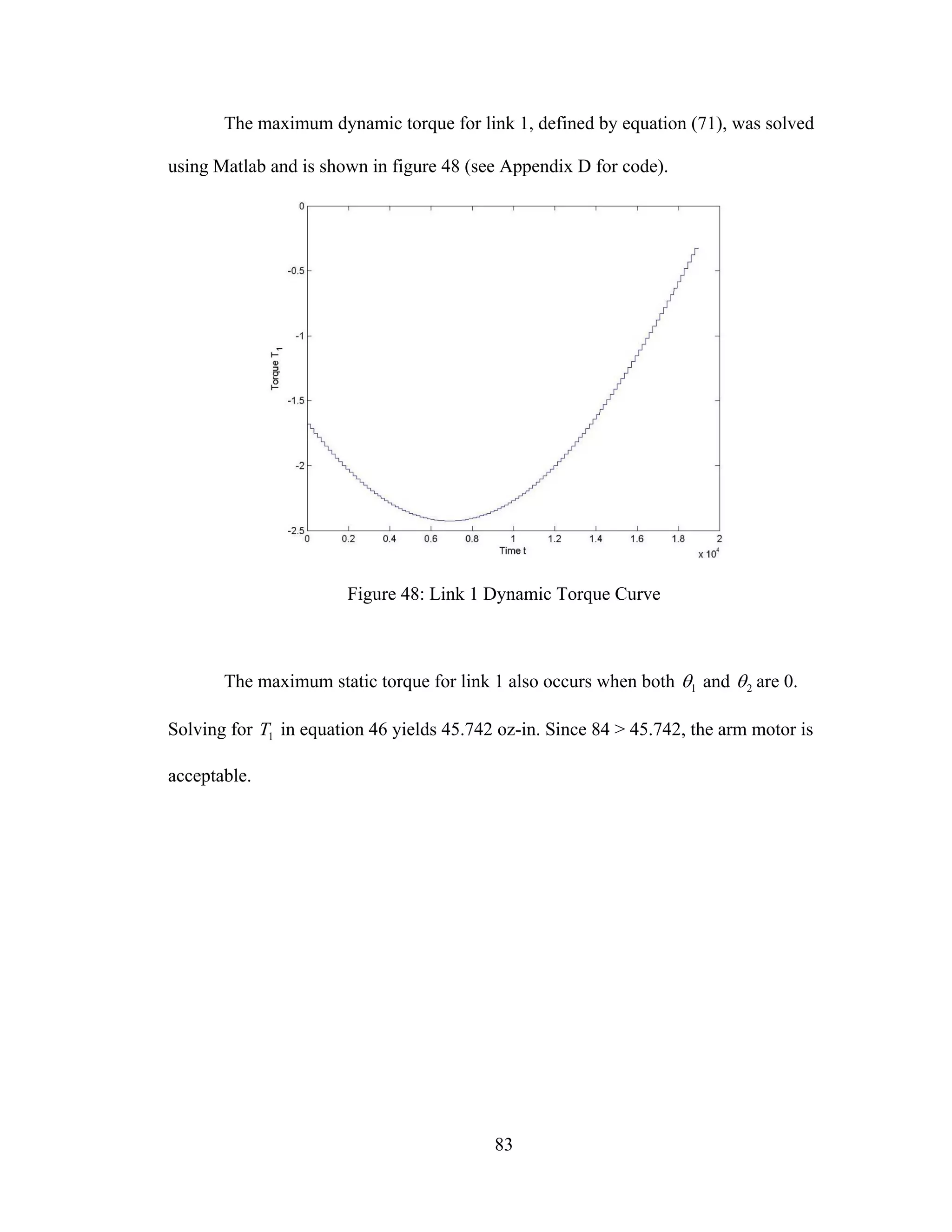
48: Link 1 Dynamic Torque Curve................................................................................... 83
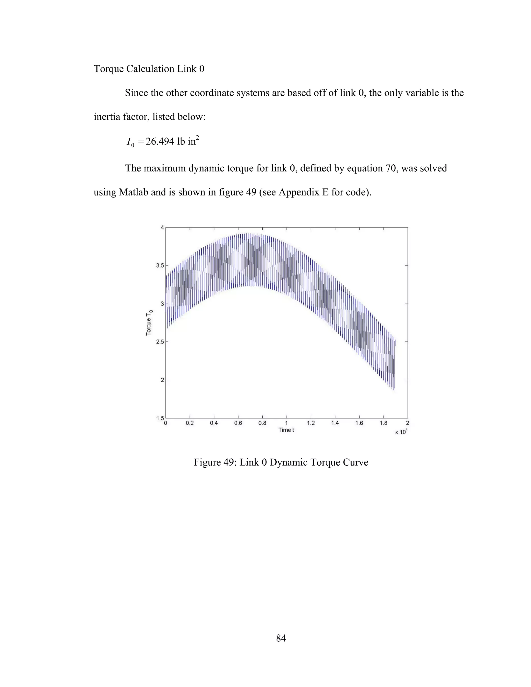
49: Link 0 Dynamic Torque Curve................................................................................... 84
50: FET-3 Controller Board Diagram............................................................................... 87
51: Parallel Port Setup for FET-3 Controller Interface..................................................... 88
52: CNC Command Line Format...................................................................................... 89
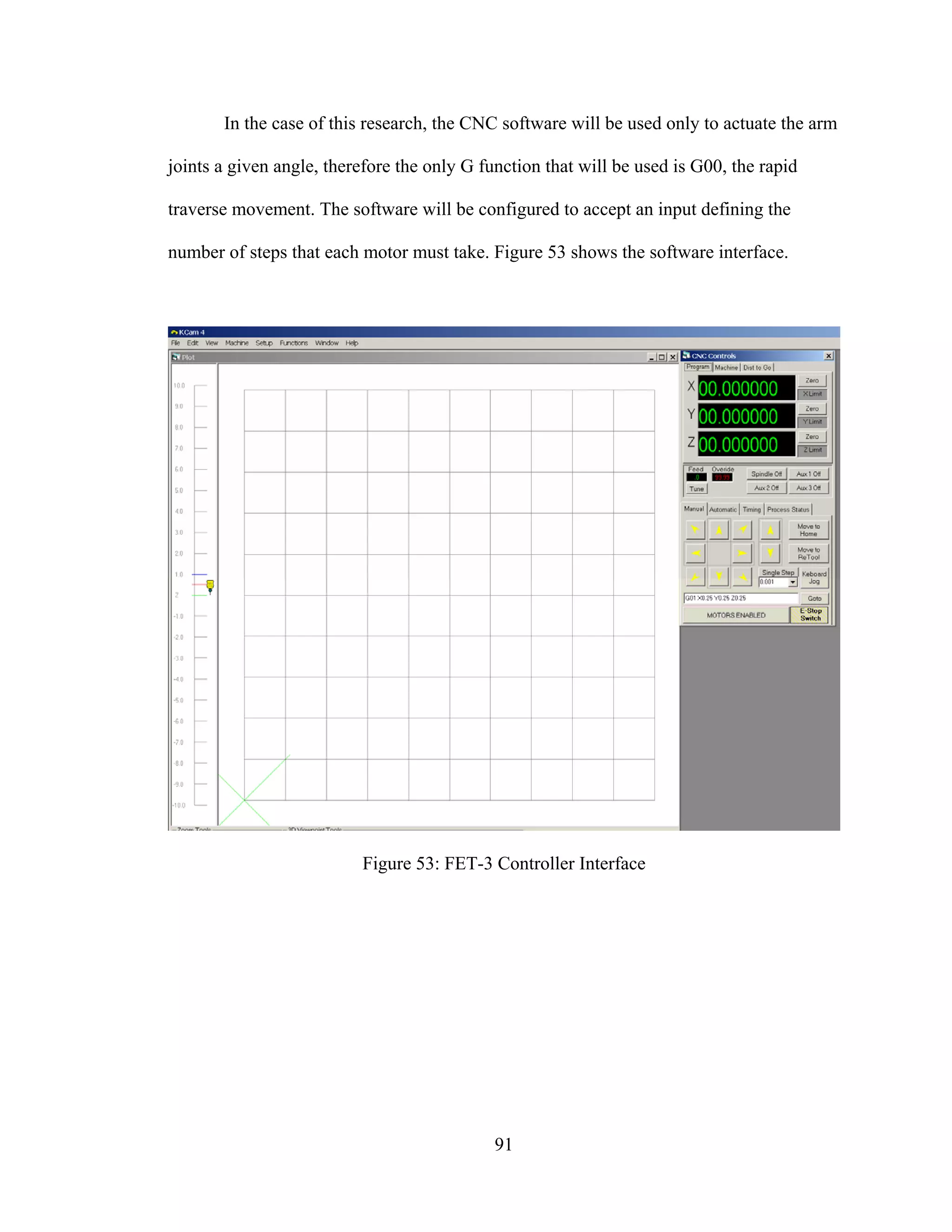
53: FET-3 Controller Interface ......................................................................................... 91
54: Standard Parallel Port Pinout [2] ................................................................................ 92
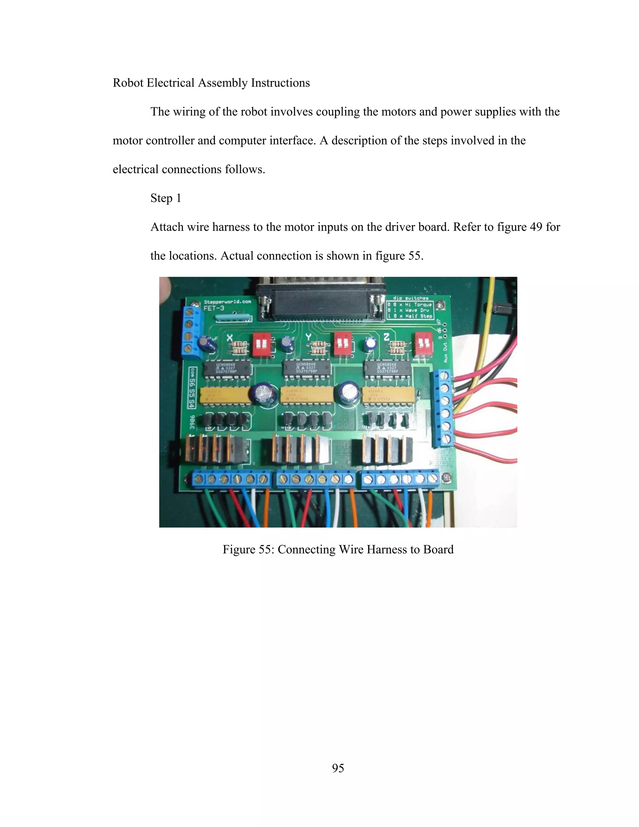
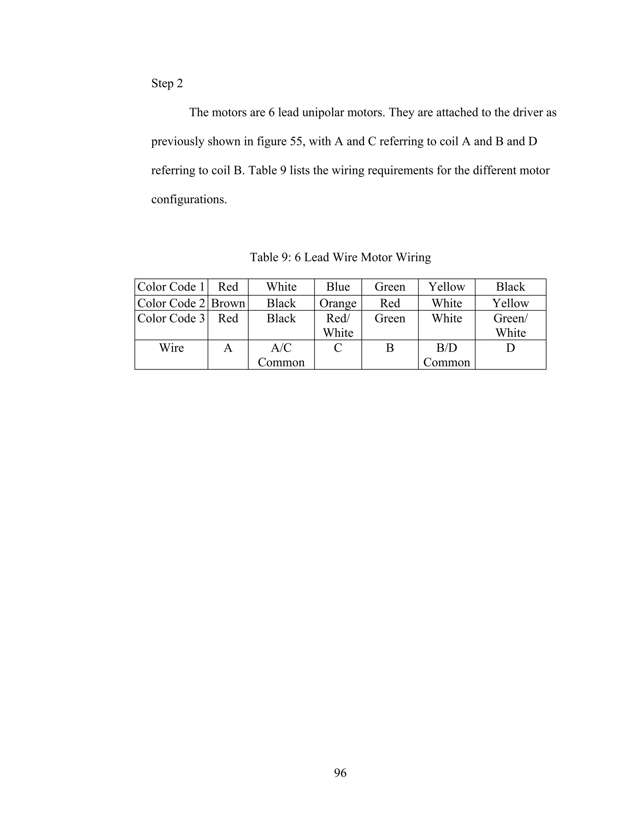
55: Connecting Wire Harness to Board ............................................................................ 95
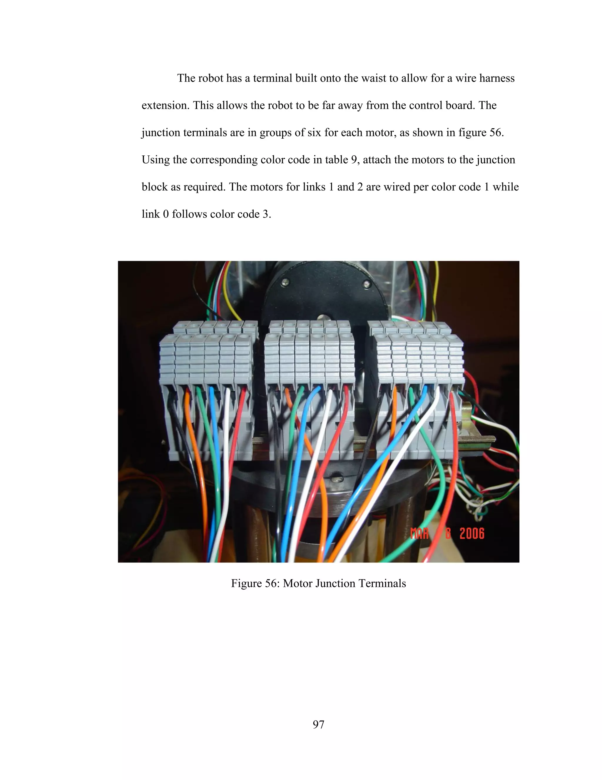
56: Motor Junction Terminals........................................................................................... 97](https://image.slidesharecdn.com/designcontrolandimplementationofathreelink-190121102715/75/Design-control-and-implementation-of-a-three-link-8-2048.jpg)

![3
CHAPTER II
REVIEW OF ROBOTIC SYSTEMS
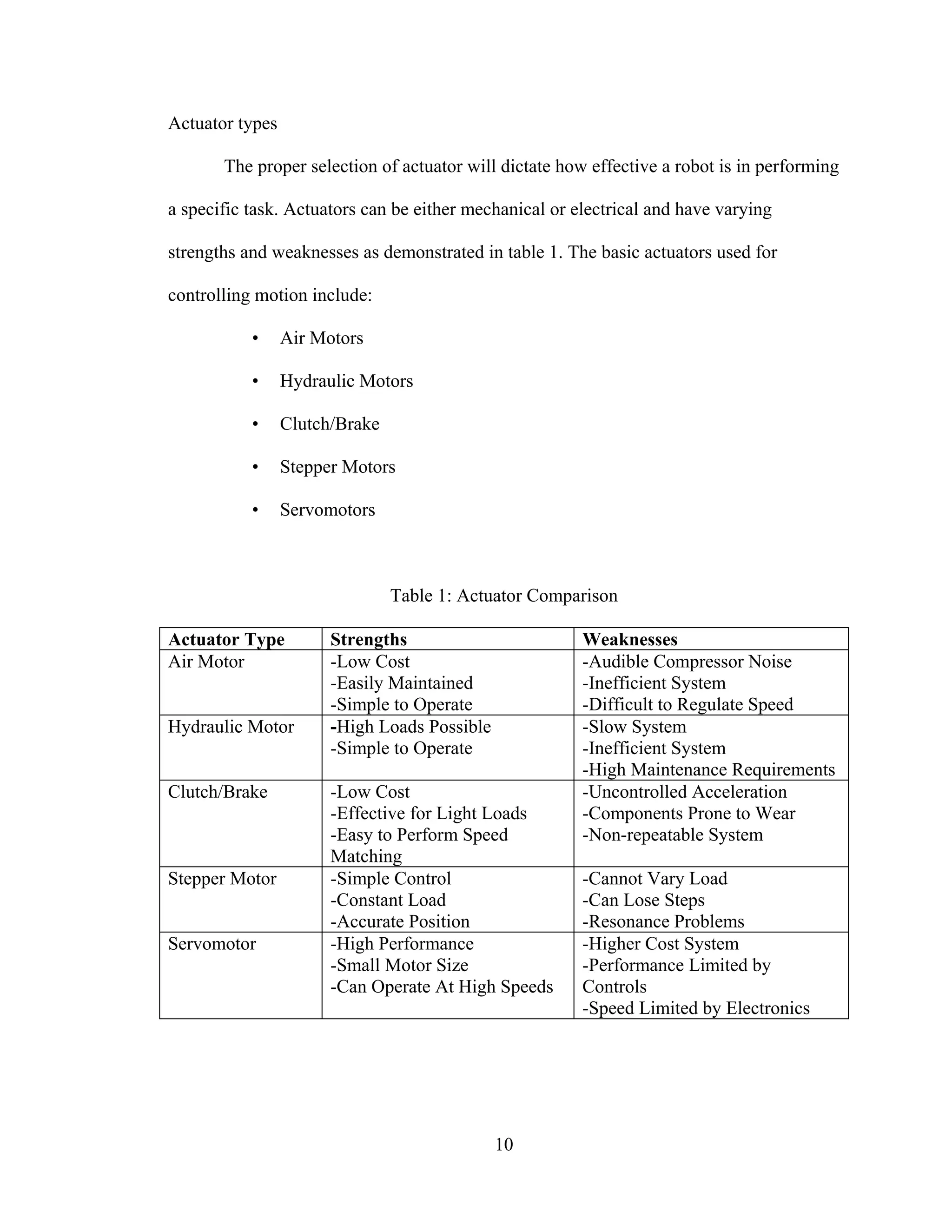
Typically, robots are used to perform jobs that are difficult, hazardous or
monotonous for humans. They lift heavy objects, paint, weld, handle chemicals, and
perform assembly work for days at a time without suffering from fatigue. Robots are
defined by the nature of their movement. This section describes the following
classifications of robots [1,4]:
• Cartesian
• Cylindrical
• Polar
• Articulated
• SCARA
Cartesian Robot [6,1,4]
Cartesian, or gantry, robots are defined by movement limited by three prismatic
joints (figure 1). The workspace is defined by a rectangle resulting from the coincident
axes.](https://image.slidesharecdn.com/designcontrolandimplementationofathreelink-190121102715/75/Design-control-and-implementation-of-a-three-link-11-2048.jpg)
![6
Articulated Robot
Substituting a revolute joint for the final prismatic joint turns the arm into an
articulated arm. Any robot whose arm has at least three rotary joints is considered to
be an articulated robot (figure 4). The workspace is a complex set of intersecting
spheres.
Figure 4: Articulated Robot Motion [2]
It can be seen that the required workspace weighs heavily in the selection of a robotic
system. Figure 5 makes a comparison of the previously described robotic systems.](https://image.slidesharecdn.com/designcontrolandimplementationofathreelink-190121102715/75/Design-control-and-implementation-of-a-three-link-14-2048.jpg)
![7
Figure 5: Robot Comparison Chart [4]](https://image.slidesharecdn.com/designcontrolandimplementationofathreelink-190121102715/75/Design-control-and-implementation-of-a-three-link-15-2048.jpg)

![12
Permanent Magnet Steppers
The permanent magnet (PM) motor (shown in figure 7) has a permanent magnet
attached to the rotor. It is a relatively low speed, low torque device with large step angles
of either 45° or 90°. Its simple construction and low cost make it an ideal choice for non-
industrial applications, such as a line printer wheel positioner.
Figure 7: Permanent Magnet Motor[1]
Unlike the other stepper motors, the PM motor rotor has no teeth and is designed
to be magnetized at a right angle to its axis. The above illustration shows a simple, 90°
PM motor with four phases (A-D). Applying current to each phase in sequence will cause
the rotor to rotate by adjusting to the changing magnetic fields. A 45° angle can be
obtained by energizing two adjacent poles simultaneously.
Variable Reluctance Steppers
The variable reluctance motor does not use a permanent magnet. As a result, the
motor rotor can move without constraint or detent torque. This type of construction is
good in non-industrial applications that do not require a high degree of motor torque,
such as the positioning of a micro slide.](https://image.slidesharecdn.com/designcontrolandimplementationofathreelink-190121102715/75/Design-control-and-implementation-of-a-three-link-20-2048.jpg)
![13
The variable reluctance motor shown in figure 8 has four stator pole pairs set 15°
apart. Current applied to pole A through the motor winding causes a magnetic attraction
that aligns the rotor to pole A. Energizing stator pole B causes a 15° rotation to align with
pole B. This process will continue with pole C and back to A in a clockwise direction.
Reversing this procedure (C to A) would result in a counterclockwise rotation.
Figure 8: Variable Reluctance Motor[1]](https://image.slidesharecdn.com/designcontrolandimplementationofathreelink-190121102715/75/Design-control-and-implementation-of-a-three-link-21-2048.jpg)
![14
Hybrid Steppers
Hybrid motors combine the best characteristics of the variable reluctance and
permanent magnet motors. They are constructed with multi-toothed stator poles and a
permanent magnet rotor. Standard hybrid motors have 200 rotor teeth and rotate at 1.8º
step angles. Other hybrid motors are available in 0.9º and 3.6º step angle configurations.
Because they exhibit high static and dynamic torque and run at very high step rates,
hybrid motors are used in a wide variety of industrial applications. Figure 9 shows the
configuration of a hybrid stepper motor.
Figure 9: Hybrid Stepper Motor[1]
Motor Windings
Hybrid stepper motor stators can be wound in two ways, unifilar and bifilar. The
windings affect how the current flows through the motor and, in turn how the motor
performs.](https://image.slidesharecdn.com/designcontrolandimplementationofathreelink-190121102715/75/Design-control-and-implementation-of-a-three-link-22-2048.jpg)
![15
Unifilar Windings
Unifilar has only one winding per stator pole. Stepper motors with a unifilar
winding will have 4 lead wires. Figure 10 is a wiring diagram that illustrates a typical
unifilar motor:
Figure 10: Unifilar Motor Winding [1]](https://image.slidesharecdn.com/designcontrolandimplementationofathreelink-190121102715/75/Design-control-and-implementation-of-a-three-link-23-2048.jpg)
![16
Bifilar Windings
Bifilar wound motors means that there are two identical sets of windings on each
stator pole. This type of winding configuration simplifies operation in that transferring
current from one coil to another wound in the opposite direction, will reverse the rotation
of the motor shaft. To accomplish this feat in a unifilar application would require the
current to physically reverse its direction along the same winding. The most common
wiring configuration for bifilar wound stepper motors is 8 leads because it offers the
flexibility of either a series or parallel connection. There are, however, many 6-lead
stepping motors available for series connection applications. Figure 11 demonstrates both
the 6 and 8 lead wiring diagrams.
Figure 11: Bifilar Motor Windings. Left: 6 Lead Motor. Right: 8 Lead Motor [1]
Step Modes
Steppers may be stepped one of three ways depending on how and when the
stators are energized. The step modes are:
• Full step mode
• Half step mode](https://image.slidesharecdn.com/designcontrolandimplementationofathreelink-190121102715/75/Design-control-and-implementation-of-a-three-link-24-2048.jpg)

![19
Figure12:TorqueDegradationwithStepDivision[2]](https://image.slidesharecdn.com/designcontrolandimplementationofathreelink-190121102715/75/Design-control-and-implementation-of-a-three-link-27-2048.jpg)

![23
Brushless DC Motor [17]
A brushless DC motor replaces the commutator and brushes with an electronic
controller. This controller maintains the proper current in the stationary coils. Figure 15
shows a basic diagram of a brushless DC motor.
Figure 15: Brushless DC Motor
It should be noted that the internal layout of a brushless DC motor looks very
similar to a permanent magnet stepper, yet a brushless motor relies on a feedback device
such as a Hall Effect sensor to keep track of the position of the rotor. This provides for
precise speed control. The brushless DC motor has a much higher initial cost than a
conventional DC motor, but these costs can usually be justified by the increased
performance and elimination of the maintenance needed to replace the brush contacts.
Induction AC Motor](https://image.slidesharecdn.com/designcontrolandimplementationofathreelink-190121102715/75/Design-control-and-implementation-of-a-three-link-31-2048.jpg)
![29
Closed Loop [3]
A closed loop system operates as shown in figure 20. A command signal is sent to
the motor and a feedback signal is returned to the controller indicating the motor’s
current state. The controller compares the command and feedback signals and adjusts its
output accordingly.
Figure 20: Closed Loop System
Closed loop systems are effective when the process demands control over a
variety of complex motion profiles. Closed loop allows for precise control over speed and
position through the use of feedback devices such as tachometers, encoders, or resolvers.
Because of additional components required, a closed loop system is more complex and
can cost more initially; but these issues are offset by the added degrees of control.
The low power command signal is amplified by the servo controller to produce
movement of the motor and load. As the motor moves the load, an appropriate feedback
signal is generated and returned to the positioning controller. The controller in turn
evaluates this signal and determines whether or not the motor is operating properly. If the
command signal and feedback signal are not equal, the controller will correct the position
signal until the difference between the two is zero.
FEEDBACK
INPUT CONTROL DRIVER MOTOR SENSOR
OUTPUT](https://image.slidesharecdn.com/designcontrolandimplementationofathreelink-190121102715/75/Design-control-and-implementation-of-a-three-link-37-2048.jpg)
![30
Motor Driver Circuits
The electric current produced by the control circuit is normally not high enough to
induce the necessary torque for motor rotation. For this reason, driver circuits are
employed. They manage the higher currents required by the motor and convert a digital
control signal from the controller into a movement by the motor. Drivers also manage the
direction that the current is flowing to produce clockwise or counterclockwise motion.
Types of Stepper Motor Drivers
Generally, there are three basic types of stepper driver technologies, they are:
• Unipolar
• Resistance/limited
• Bipolar chopper.
All drivers utilize a "translator" to convert the step and direction signals from the
indexer into electrical pulses to the motor. The essential difference between driver
options is the “switch set,” or the circuit that energizes the motor windings. Figure 21
shows the flow of information from controller to stepper motor.
Figure 21: Information Flow Between Driver and Motor[1]](https://image.slidesharecdn.com/designcontrolandimplementationofathreelink-190121102715/75/Design-control-and-implementation-of-a-three-link-38-2048.jpg)
![31
Unipolar Drive
A unipolar drive consists of a winding with a center-tap, or two separate windings
per phase, which limits the current flow to one direction. The direction is reversed by
moving the current from one half of the winding to the other half using two switches per
phase, as shown in figure 22. Therefore, the switch set of a unipolar drive is simple and
inexpensive. However, the unipolar drive utilizes only half the available conducting wire
volume on the winding. As a result, the torque output of a unipolar driver is reduced by
nearly 40% when compared to other technologies. Unipolar drivers are useful in
applications that operate at relatively low step rates.
Figure 22: Current Flow Through Unipolar Drive[5]](https://image.slidesharecdn.com/designcontrolandimplementationofathreelink-190121102715/75/Design-control-and-implementation-of-a-three-link-39-2048.jpg)
![32
Resistance/Limited Drive
Resistance/Limited (R/L) drivers are simple and inexpensive. The driver limits
the current by supply voltage and the resistance of the winding. High speed performance
is improved by increasing the supply voltage. This increased supply voltage in the R/L
drive must be accompanied by an additional resistor in series with the winding to limit
the current to the previous level (figure 23). This resistor, called a dropping resistor, is
added to maintain a useful increase in speed. The drawback of this method is the power
loss in the dropping resistors. This process also produces an excessive amount of heat and
must rely on a DC power supply for its current source.
Figure 23: R/L Driver Circuit [5]](https://image.slidesharecdn.com/designcontrolandimplementationofathreelink-190121102715/75/Design-control-and-implementation-of-a-three-link-40-2048.jpg)
![33
Bipolar Chopper Drive
Bipolar chopper drivers are by far the most widely used drivers for industrial
applications. Although they are typically more expensive to design, they offer high
performance and high efficiency. This driver employs two different principles to control
the current flow to the motor windings: a bipolar switch set and current chopping. Both
are explained in this section.
A Bipolar drive, as the name implies, switches the current direction on a single
winding by shifting the voltage polarity across the terminals. The polarity switch is
accomplished using four switches configured as shown in figure 24. This configuration is
called an H-bridge.
Figure 24: H-bridge [5]](https://image.slidesharecdn.com/designcontrolandimplementationofathreelink-190121102715/75/Design-control-and-implementation-of-a-three-link-41-2048.jpg)
![35
Additionally, these drivers use a four transistor H-bridge with recirculating diodes
and a sense resistor that maintains a feedback voltage proportional to the motor current.
Motor windings, using a bipolar chopper driver, are energized to the full supply level by
turning on one set of the switching transistors. The sensing resistor develops a voltage
with the linear rise in current, which is monitored by a comparator, until the required
level is reached. At this point the top switch opens and the current in the motor coil is
maintained via the bottom switch and the diode. Current decay occurs until a preset
position is reached and the process starts over. This "chopping" effect of the supply is
what maintains the correct current voltage to the motor at all times (figure 25).
Figure 25: Chopper Pulse Chart [5]](https://image.slidesharecdn.com/designcontrolandimplementationofathreelink-190121102715/75/Design-control-and-implementation-of-a-three-link-43-2048.jpg)
![36
Figure 26 illustrates an H-bridge configured as a constant current chopper.
Depending on how the H-bridge is switched during the turn-off period, the current will
either recirculate through one transistor and one diode (path 2), giving the slow current
decay, or recirculate back through the power supply (path 3).
Figure 26: Bipolar Chopper Schematic [5]
Servo Drivers [6]
Servo motors are controlled using electronic pulses. Normally, transistors are
employed to regulate the pulses. There are three basic transistor circuits used for
servomotor control; linear, pulse width modulated and pulse frequency modulated.
Linear Driver](https://image.slidesharecdn.com/designcontrolandimplementationofathreelink-190121102715/75/Design-control-and-implementation-of-a-three-link-44-2048.jpg)
![39
Parallel Port [7] [8]
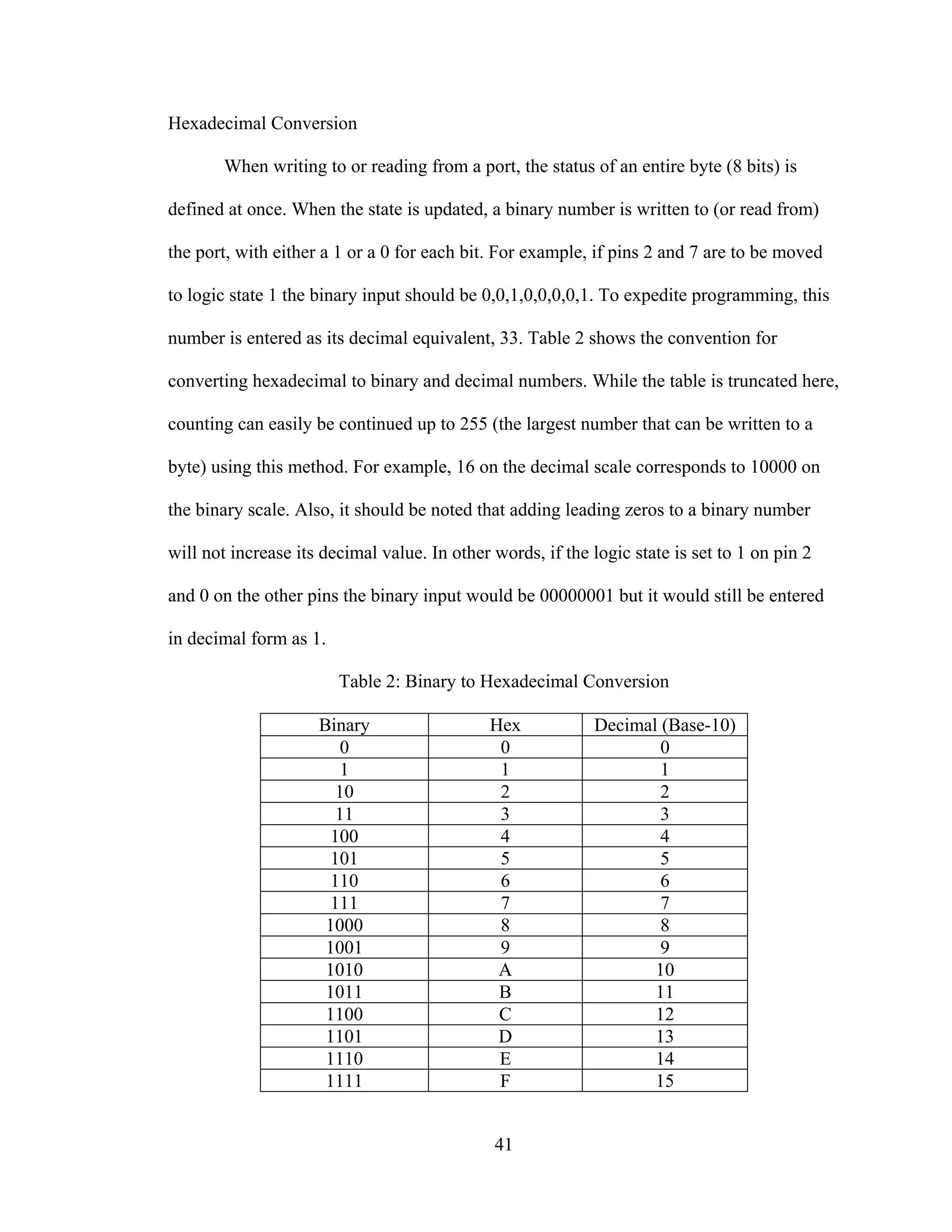
When a PC sends data to a printer or other device using a parallel port, it can send
8 bits of data (1 byte) simultaneously. These 8 bits are being transmitted in parallel to
each other, as opposed to the same eight bits being transmitted serially, 1 bit at a time,
through a serial port. The standard parallel port is capable of sending 50 to 100 kilobytes
of data per second. Figure 29 shows the layout of a common configuration of parallel
port, DB25, which has 25 pins.
Figure 29: Layout of DB25 Parallel Port[1]
Following is a description of the pins:
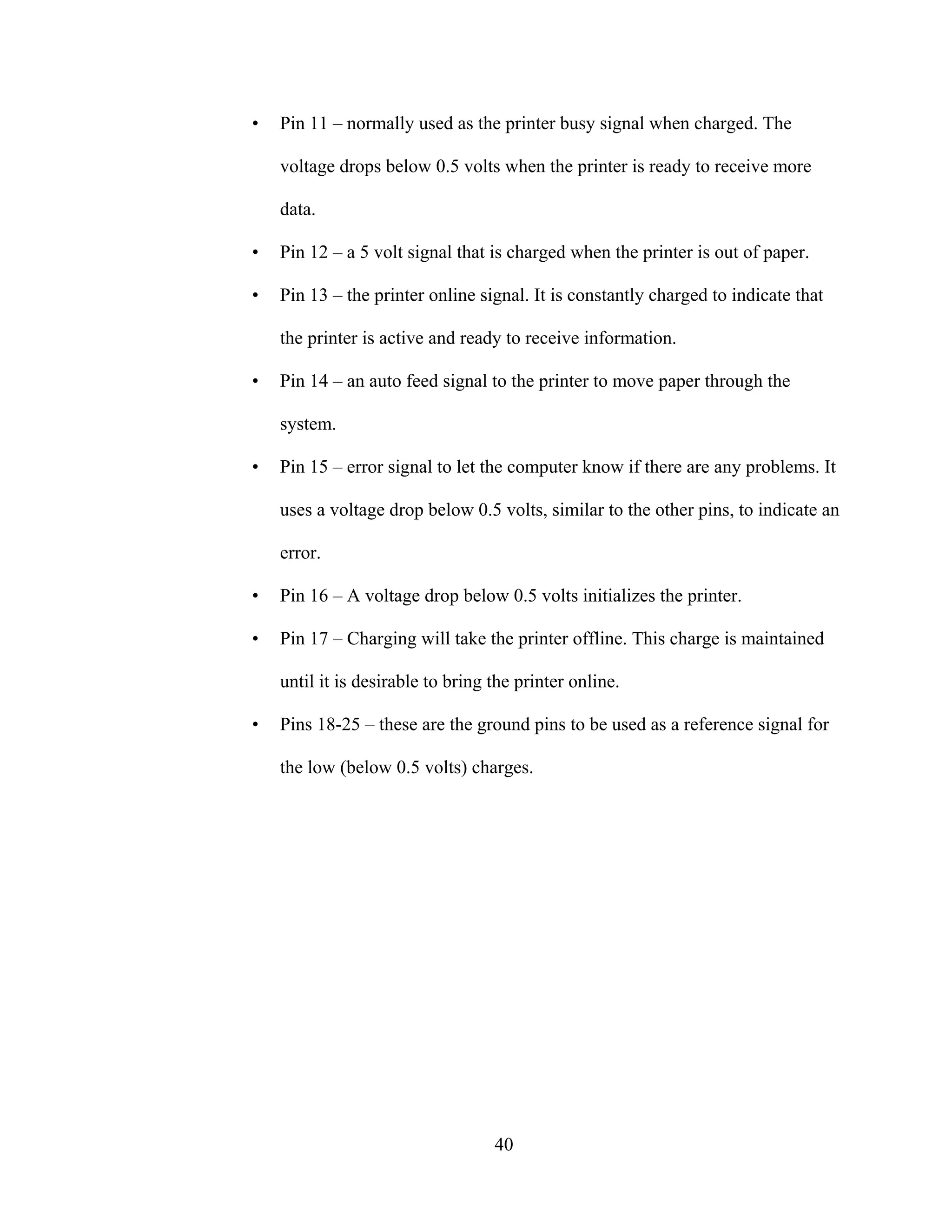
• Pin 1 – maintains a voltage between 2.8 and 5 volts, called the strobe
signal. When data is sent to the printer the voltage drops below 0.5 volts as
the computer sends a byte of data.
• Pins 2 through 9 – used to exchange data between the PC and receiving
entity. A simple method is used to indicate whether a bit has a value of 1
or 0. A charge of 5 volts is sent through means a particular pin has a bit
value of 1. No charge indicates a value of 0.
• Pin 10 – operates in a similar fashion to Pin 1. A voltage drop indicates to
the computer to confirm that the data has been received. This is called the
acknowledge signal.](https://image.slidesharecdn.com/designcontrolandimplementationofathreelink-190121102715/75/Design-control-and-implementation-of-a-three-link-47-2048.jpg)

![54
• n
n
r center of mass wrt to nth
frame
• )0,,,( zyx gggg = is the gravity row vector expressed in base frame
The potential energy of the robot arm is then:
∑ ∑= =
−==
n
n
n
n
n
nn
nn rTgmPP
0 0
0 ])([ (39)
Which is a function of nq .
Lagrange Function
In order to simplify the solution, the dynamic equations can be determined using
Lagrangian mechanics. The Lagrange function allows the forces to be determined using
the system’s energy. This eliminates the need to solve for acceleration components. Since
energy is a scalar quantity, it also makes the equations easier to manage. The Lagrangian
function takes the form of:
[ ]∑∑∑ ∑= = = =
+=−=
i
n
n
j
n
k
i
n
n
n
nnkj
T
nknnj rTgmqqUJUTrPKL
1 1 1 1
0
)()(
2
1
&& (40)
Where L is the Lagrange – Euler equation:
n
nn q
L
q
L
dt
d
τ=
∂
∂
−
∂
∂
)(
&
(41)
j
j
jn
i
nj
j
i
nj
j
k
j
m
mk
T
jnj
m
jk
i
nj
j
k
k
T
jnjjk rUgmqqUJ
q
U
TrqUJUTr ∑∑∑∑∑∑ == = == =
−
∂
∂
+=
1 11
)()( &&&& (42)
And:
• K: Total kinetic energy of robot
• P: Total potential energy of robot
• nq : Joint variable of nth
joint
• nq& : First time derivative of nq](https://image.slidesharecdn.com/designcontrolandimplementationofathreelink-190121102715/75/Design-control-and-implementation-of-a-three-link-62-2048.jpg)
![58
Inverse Solution
The inverse solution requires determining the necessary link rotations and
transformations needed to achieve the desired location and orientation of the end effector.
In some cases this can lead to multiple solutions for a movement. There have been
numerous studies performed on determining the most efficient orientation of the joints,
some of which will be referenced in this section. An example of an inverse solution is
shown below, using a proprietary algorithm from New River Kinematics. Figure 35
shows the robot arm at [0,0,0] and the desired end point in space at [7, -1, 3]. Figure 36
shows the robot arm translated to the point. A plot of the joint motions during the inverse
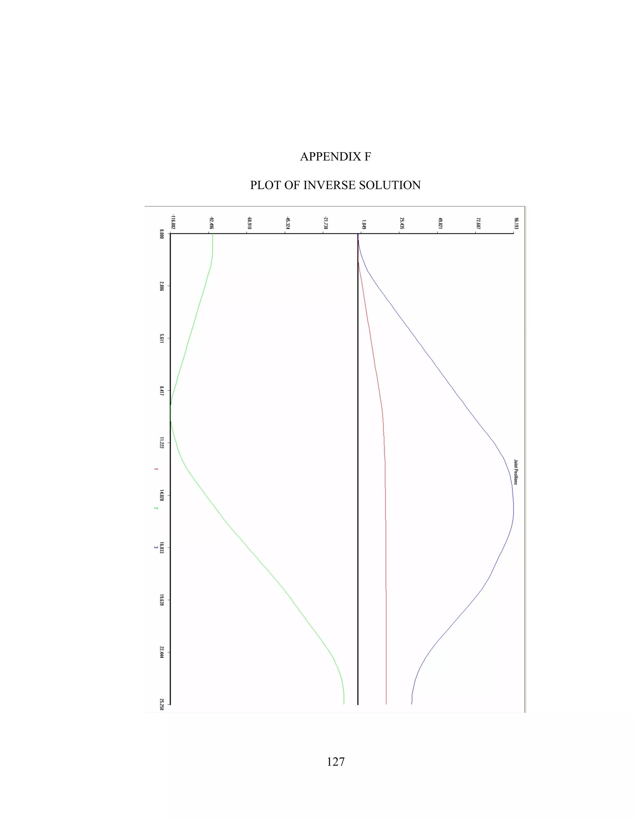
solution is included in Appendix F.
Figure 35: Robot arm before inverse solution](https://image.slidesharecdn.com/designcontrolandimplementationofathreelink-190121102715/75/Design-control-and-implementation-of-a-three-link-66-2048.jpg)
![59
Figure 36: Robot arm translated to end point
Elements of the inverse solution include path planning, curve tracking and the
configuration space. A brief commentary on these concepts follows.
Path Planning
The goal of path planning algorithms is to generate the most efficient arrangement
of the link frames, taking into account any physical obstacles and system limitations.
Configuration Space
Problems that arise in the motion planning process can be related to the physical
design of the robot of the restrictions of the workspace [11]. For example, as the number
of available degrees of freedom increase, so do the possible solutions to the inverse
transformation. Also, obstacles in the workspace, which includes links of the robot arm,
can add difficulty to the solution.](https://image.slidesharecdn.com/designcontrolandimplementationofathreelink-190121102715/75/Design-control-and-implementation-of-a-three-link-67-2048.jpg)
![60
Curve Tracking
When a robot has to follow a complicated path or if the reference point is moving
with time, an open-loop controller is sometimes not sufficient. Curve tracking and path
planning methods are a vast area of study. This section describes some closed-loop
control methods for tracking a robots movement.
Potential Energy Method
[12] outlines using a potential energy field approach to guiding the robot.
Sometimes it is desirable for the robot to stay on a certain curve instead of following a
reference point. The exact position at a given time is not important, as long as it is
somewhere on this desired curve. To solve this problem, a virtual potential field is
constructed around the desired curve, such that the potential energy is minimal
everywhere on the desired curve, and increases with the deviation from the desired curve.
The system can then follow the path of steepest descent to find its commanded position.
[13] extends the use of this method to add control terms that are power-
continuous but change the distribution of kinetic energy over the various directions to
obtain asymptotic convergence.
Orthogonal Decomposition Control
[14] describes using a vision system to guide the robot. The automatic input is
accomplished using a method called Orthogonal Decomposition Control. The center of
the camera is defined by the vector r. At each sample point, the ji
rr
− vector coordinate
frame is established, where i
r
is a unit vector tangent to the curve and j
r
is the normal unit
vector. The objective is to control the velocity error signal based on the vector tangent to
the curve and the position error signal based on the normal vector.](https://image.slidesharecdn.com/designcontrolandimplementationofathreelink-190121102715/75/Design-control-and-implementation-of-a-three-link-68-2048.jpg)
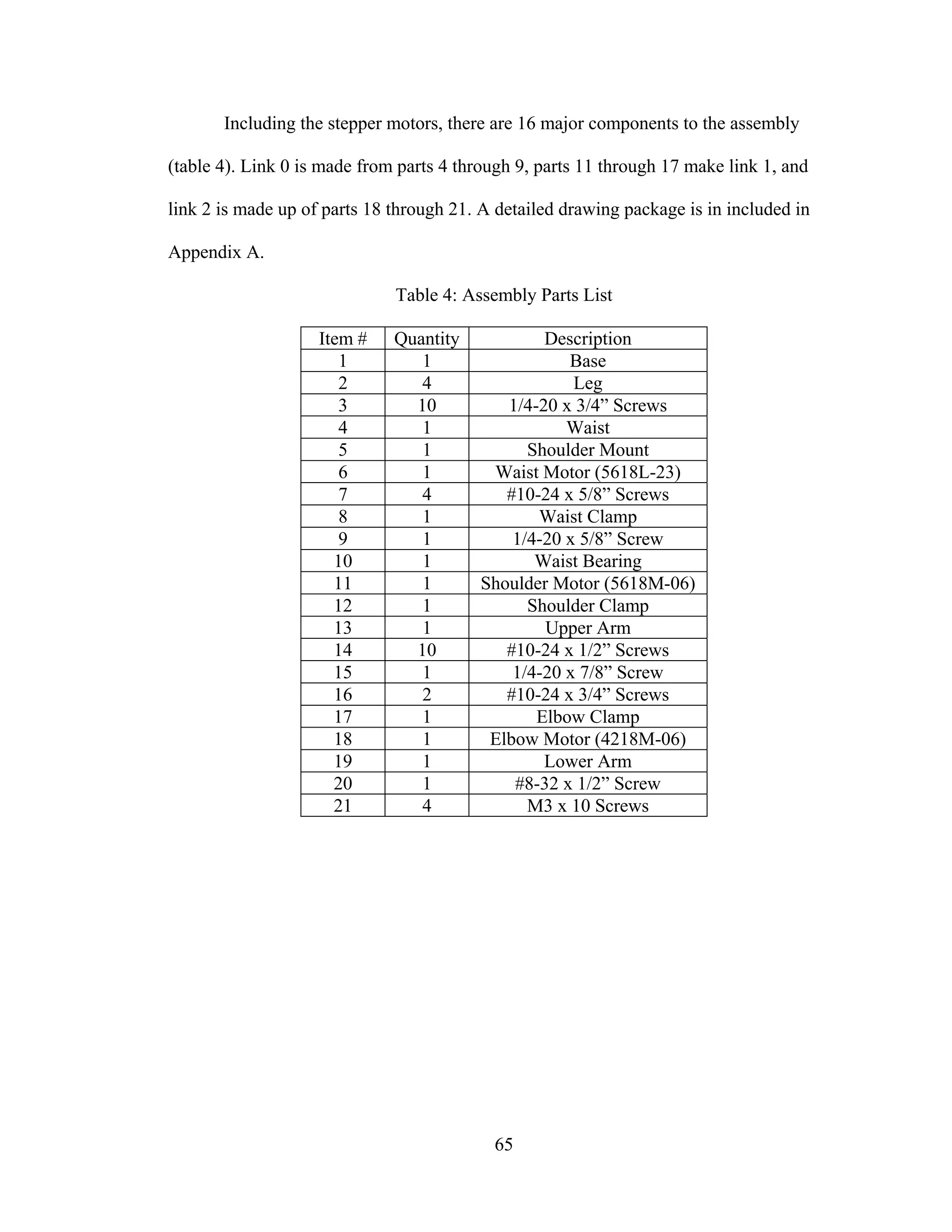
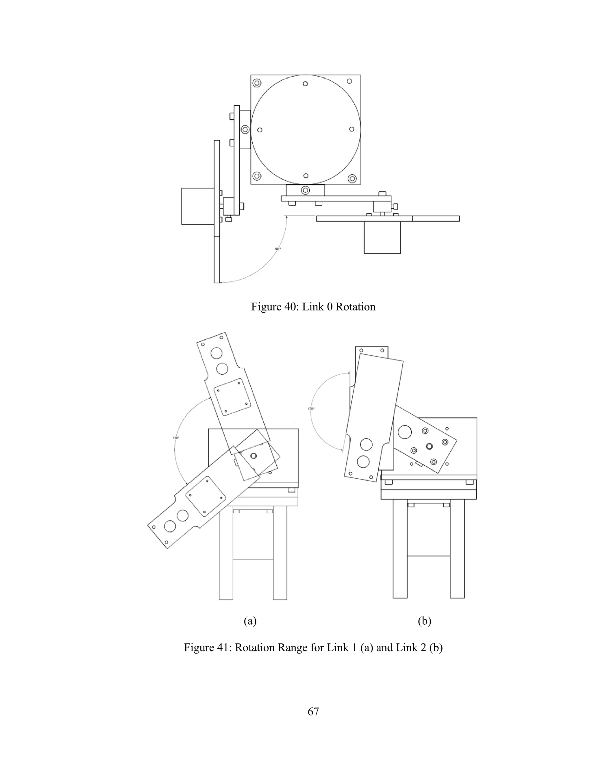
![66
Robot Workspace
The workspace is defined in figures 39 through 41. The reaching length is 4.5
inches, the height is 15.0 inches and the total rotation at the waist (link 0) is 90°, defined
by a range of [0,90] (Figure 40). Link 1 is permitted to have a range of [-40,70] (Figure
41 (a)), for a total rotation of 110° and link 2 is allowed a range of [-80,90] (Figure 41
(b)), for a total rotation of 170°.
Figure 39: Robot Arm Reach Dimensions](https://image.slidesharecdn.com/designcontrolandimplementationofathreelink-190121102715/75/Design-control-and-implementation-of-a-three-link-74-2048.jpg)
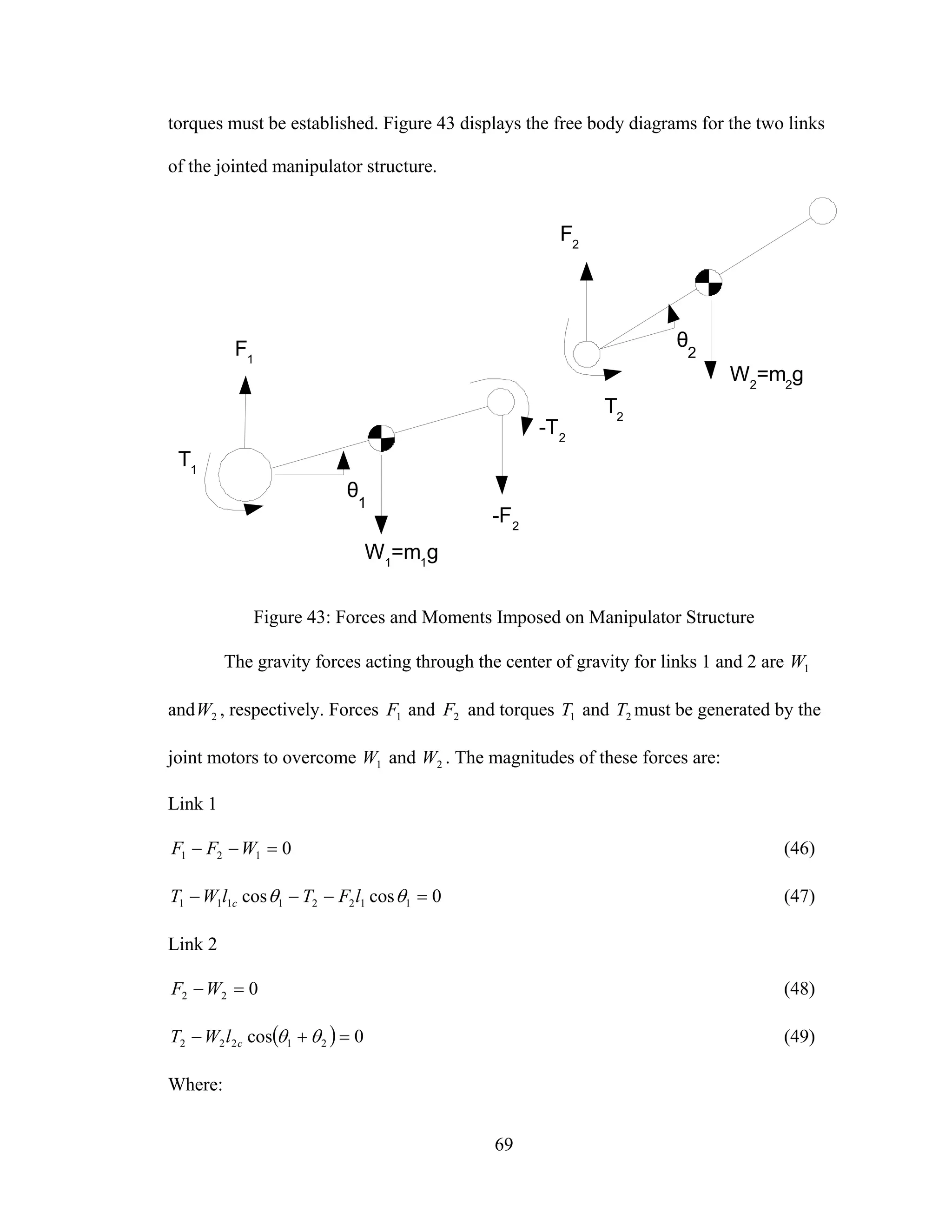
![70
• ( )gmmF 211 +=
• gmF 22 =
• ( )[ ]1121221111 coscoscos θθθθ llgmglmT cc +++=
• ( )21222 cos θθ += cglmT
• =1m 1.116 lbs. = 17.86 oz.
• =2m 0.217 lbs. = 3.470 oz
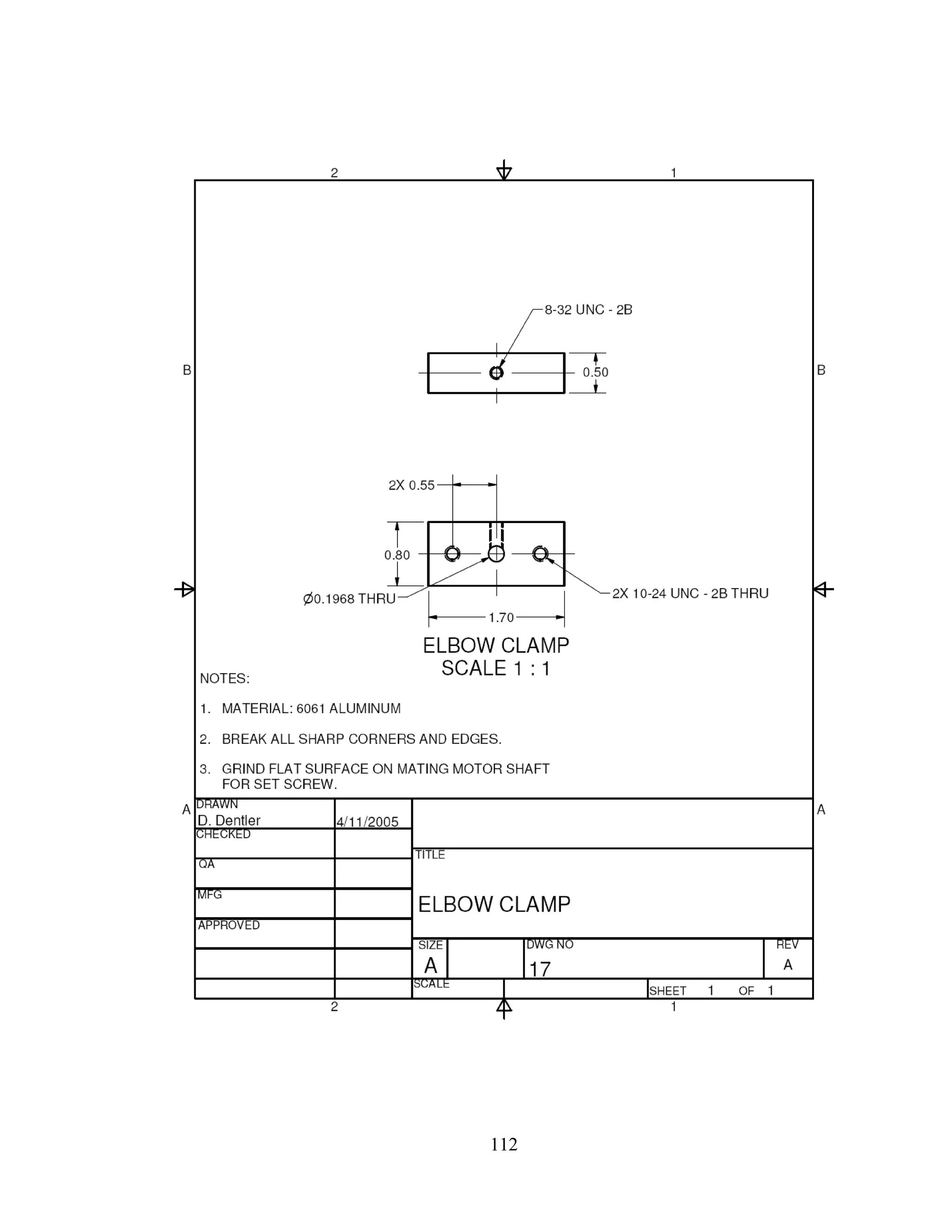
Mass 1m includes the weight of the shoulder clamp (item 12), the elbow clamp
(item 17), and the elbow motor (item 18). The torques, 1T and 2T , required to overcome
gravity forces, can become very large in magnitude. However, these magnitudes can be
controlled during the design phase by performing actions such as choosing low mass
materials, shaping the link to move the center of gravity closer to the joint axis of
rotation, or adding a counterbalance to the link.
System Stability
In order to prevent the robot from tipping over when the arms are outstretched,
the torque generated by links 1 and 2 at the maximum reaching distance must be less than
the counterbalance torque from the robots base.](https://image.slidesharecdn.com/designcontrolandimplementationofathreelink-190121102715/75/Design-control-and-implementation-of-a-three-link-78-2048.jpg)
![72
Dynamic Torque Analysis
In order to calculate the forces required to drive the links at the desired velocity
and acceleration profiles, dynamic equations must be used. These equations are related to
the Lagrange equations previously described.
Dynamic Torque Link 0
For link 0 the kinetic and potential energy are expressed as
2
2
0
00
•
=
θ
IK 00 =V (50)
The torque 00T , which has to be developed by the waist joint motor to support the link 0
motion, is determined by the Lagrange equation
0
0
0
0
00
θθ ∂
∂
−
⎟⎟
⎟
⎠
⎞
⎜⎜
⎜
⎝
⎛
∂
∂
= •
KK
dt
d
T or 0000
••
= θIT (51)
Dynamic Torque Link 1
For link 1, the position vector gr1 , the origin of which is at the center 1O , and the
velocity gv1 of the center of gravity of link 1 are
( ) ( ) ( )[ ]kjilr cg 1101011 sinsinsincoscos θθθθθ ++= (52)
( ) ( )
( ) ( )
( ) }]cos[
]sinsincoscos[
]sincoscossin[{
01
110010
110010111
k
j
ilrv cgg
•
••
•••
+
++
+−==
θθ
θθθθθθ
θθθθθθ
(53)](https://image.slidesharecdn.com/designcontrolandimplementationofathreelink-190121102715/75/Design-control-and-implementation-of-a-three-link-80-2048.jpg)
![74
Dynamic Torque Link 2
For link 2, the position vector of center of gravity of link 2 relative to 1O is
( )[ ]
( )[ ]
( )[ ]kll
jll
illr
c
c
cg
21211
212110
2121102
cossin
coscossin
coscoscos
θθθ
θθθθ
θθθθ
+++
+++
++=
(59)
The velocity center of gravity of link 2 is
( )
( )
( )
( )
( ) kll
jll
ll
ill
llrv
c
c
c
c
cgg
]coscos[
}sin]sinsin[
cos]coscos{[
}cos]sinsin[
sin]coscos[{
21212111
021212111
0021211
021212111
002121122
θθθθθθ
θθθθθθθ
θθθθθ
θθθθθθθ
θθθθθ
+⎟
⎠
⎞
⎜
⎝
⎛ +++
+⎟
⎠
⎞
⎜
⎝
⎛ ++−
+++
+⎟
⎠
⎞
⎜
⎝
⎛ ++−
++−==
•••
•••
•
•••
••
(60)
( )
( )
2
21
2
2221121
2
1
2
1
2
021
22
2
211211
22
122
2
2
cos2
]cos
coscos2cos[
⎟
⎠
⎞
⎜
⎝
⎛ ++⎟
⎠
⎞
⎜
⎝
⎛ ++
+++
++=⋅=
•••••
••
θθθθθθ
θθθθ
θθθθ
cc
c
cggg
lll
ll
lllvvv
(61)](https://image.slidesharecdn.com/designcontrolandimplementationofathreelink-190121102715/75/Design-control-and-implementation-of-a-three-link-82-2048.jpg)
![75
The magnitude of angular velocity 2ω of link 2 is
cg
c
g lv
l
l
v 21
1
1
22 −=ω (62)
Where ( ) gc vll 111 is the velocity of the joint between links 1 and 2. Inserting equations
(52) and (59) produces
( ) 2
2121
2
0
2
21
1
1
21
1
1
2
2
2
)(cos
•••
+++=
⎟⎟
⎠
⎞
⎜⎜
⎝
⎛
−⎟⎟
⎠
⎞
⎜⎜
⎝
⎛
−=
θθθθθ
ω cg
c
gg
c
g lv
l
l
vv
l
l
v
(63)
Thus the kinetic energy of link 2 is
( )
( )
( )
( )}cos
)(cos)(2
]cos
coscos2cos[{
2
1
21
2
2
02
2
212
2
222211212
2
1
2
12
2
021
22
2
211211
22
122
θθθ
θθθθθθ
θθθθ
θθθθ
++
+++++
+++
++=
•
•••••
••
I
Ilmllm
lml
lllmK
cc
c
c
(64)](https://image.slidesharecdn.com/designcontrolandimplementationofathreelink-190121102715/75/Design-control-and-implementation-of-a-three-link-83-2048.jpg)
![76
And the torques in the motors of joints 0, 1, and 2, respectively, required to support
motion of link 2 are
( )
( ) ( )
( ) ( )
( ) ( ) ( )
( )
( ) ( ) ( ) 2021212
2
22
211212
1021212
2
22
21121121
11
2
12021
2
2
2
22
211211
22
12
0
2
0
2
02
]cossin
sincos[2
}cossin
]sincoscos[sin
cossin[{2}cos
]coscos2cos[{
••
••
••
•
++++
+−
++++
++++
−+++
++=
∂
∂
−
⎟⎟
⎟
⎠
⎞
⎜⎜
⎜
⎝
⎛
∂
∂
=
θθθθθθ
θθθ
θθθθθθ
θθθθθθ
θθθθθ
θθθθ
θθ
Ilm
llm
Ilm
ll
lmIlm
lllm
KK
dt
d
T
c
c
c
c
c
c
(65)
( )
( ) ( )
( ) ( ) ( ) ( )
( ) 212212
2
22212
2
0212122121
2
2
2112121121
11
2
1222
2
222212
12
2
222212
2
12
1
2
1
2
12
sin2)sin(
}cossin]cossin
sincoscossin
cossin[{cos
)cos2(
•••
•
••
••
•
−−
++++++
++++
++++
+++=
∂
∂
−
⎟⎟
⎟
⎠
⎞
⎜⎜
⎜
⎝
⎛
∂
∂
=
θθθθθ
θθθθθθθθθ
θθθθθθ
θθθθ
θθ
θθ
cc
c
cc
cc
cc
llmllm
Il
llll
lmIlmllm
Ilmllmlm
KK
dt
d
T
(66)](https://image.slidesharecdn.com/designcontrolandimplementationofathreelink-190121102715/75/Design-control-and-implementation-of-a-three-link-84-2048.jpg)
![77
( )
( ) ( ) ( )
( ) ( ) 2
12212
2
021212
2121
2
2211212
22
2
2212
2
222212
2
2
2
2
22
)sin(}cossin
]cossinsincos[{
)(cos
••
••••
•
++++
+++++
++++=
∂
∂
−
⎟⎟
⎟
⎠
⎞
⎜⎜
⎜
⎝
⎛
∂
∂
=
θθθθθθθ
θθθθθθθ
θθθ
θθ
c
cc
ccc
llmI
lllm
IlmIlmllm
KK
dt
d
T
(67)
Assuming link 0 is vertical, the potential energy is
( )[ ]{ }212112111 sinsinsin θθθθ +++= cc llmlmgV (68)
Accordingly, the gravity-related components of the torque in the actuators of joints 1 and
2 are as follows
( )[ ]{ }212112111
1
1 coscoscos θθθθ
θ
+++−=
∂
∂
−= ccg llmlmg
V
T (69)
( )[ ]2122
2
2 cos θθ
θ
+−=
∂
∂
−= cg lmg
V
T (70)
These torque components are added to the motion-related components from equations
(57), (65), and (66). The overall torques to be developed by actuators in joints 0, 1, and 2
( 0T , 1T , and 2T ) are calculated as follows](https://image.slidesharecdn.com/designcontrolandimplementationofathreelink-190121102715/75/Design-control-and-implementation-of-a-three-link-85-2048.jpg)
![78
( )
( ) ( ) ( )
( ) ( )
( ) ( ) ( ) ( )
( ) ( ) ( ) ( ) 2021212
2
22211212
1021212
2
222112
211211112111
2
11
021
2
2
2
222112
1
2
1121
2
1
2
1100201000
]cossinsincos[2
]}cossinsincos
cossincossin[cossin{2
}cos]coscos2
cos[cos{
••
••
••
+++++−
++++++
++++−
+++++
+++=++=
θθθθθθθθθ
θθθθθθθθθ
θθθθθθθ
θθθθθθ
θθ
Ilmllm
Ilml
lllmIlm
Ilml
llmIlmITTTT
cc
cc
cc
cc
c
(71)
( )
( ) ( ) ( ) ( )
( ) ( )
( )]}coscos[cos{
)sin2()sin(]}cossin
cossinsincoscossin
cossin[cossin{)cos(
)cos2(
212112111
212212
2
22212
2
021212
2121
2
22112121121
11
2
12111
2
1122
2
222212
12
2
222212
2
121
2
11112111
θθθθ
θθθθθθθθθθ
θθθθθθθθθθ
θθθθθθ
θθ
++++
−−+++
+++++++
++++++
+++++=++=
••••
••
••
cc
cc
ccc
ccc
cccg
llmlmg
llmllmI
lllll
lmIlmIlmllm
IlmllmlmIlmTTTT
(72)
( ) ( ) ( )
( ) ( )
( )]cos{
)sin(}cossin
]cossinsincos[{
)()cos(
2122
2
12212
2
021212
2121
2
2211212
22
2
2212
2
2222122222
θθ
θθθθθθθ
θθθθθθθ
θθθ
++
++++
+++++
++++=+=
••
••••
c
c
cc
cccg
lmg
llmI
lllm
IlmIlmllmTTT
(73)](https://image.slidesharecdn.com/designcontrolandimplementationofathreelink-190121102715/75/Design-control-and-implementation-of-a-three-link-86-2048.jpg)
![80
Dynamic Torque Calculation
Using equations developed in equations (49) through (72), it is possible to
calculate the dynamic torque requirements of the robot arm.
Torque Calculation Link 2
As shown in figure 45, known variables in equation (48) for the arm section of the
robot, or link 2, are as follows:
• =cl2 0 in.
• =2m 0.217 lbs. = 3.47 oz.
• =2I 1.158 lb in2
• =1l 3.50 in.
Figure 45: Design Variables Link 2
Figure 41 previously defined the range of rotation angles for link 1 and 2 ( 1θ and
2θ , respectively) as [-40, 70] for link 1 and [-80, 90] for link 2. The maximum static](https://image.slidesharecdn.com/designcontrolandimplementationofathreelink-190121102715/75/Design-control-and-implementation-of-a-three-link-88-2048.jpg)
![86
Open Loop Control
Based on the transformation matrix derived in (77), a database can be constructed
which contains all of the possible end effector locations in the task space. These locations
can then be translated into a number of steps that the motors need to take in order to
rotate each joint into position.
Selection of Driver
The purpose of a stepper motor driver is to supply the current to the motor
windings through a separate power source since the required current is too high to be
supplied by a PC.
Stepper Motor Drivers
A stepper motor driver is selected according to the type of stepper motor (ie.,
unipolar or bipolar) and current/voltage requirements (refer back to table 5 for motor
info). For this application, the FET3 system, supplied by StepperWorld, was chosen. The
FET3 is a low cost driver for hobby use that proved to be very versatile to the needs of
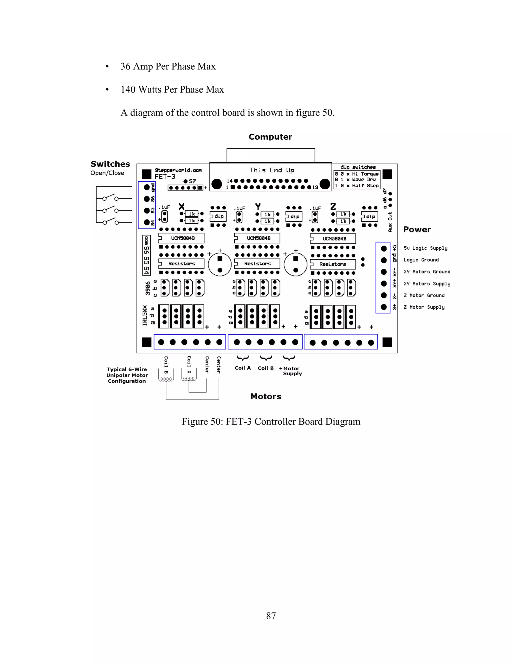
this research. The features of the FET3 board are as follows [15]:
• 3 Axis Unipolar (L/R Type Driver)
• High Current Capability
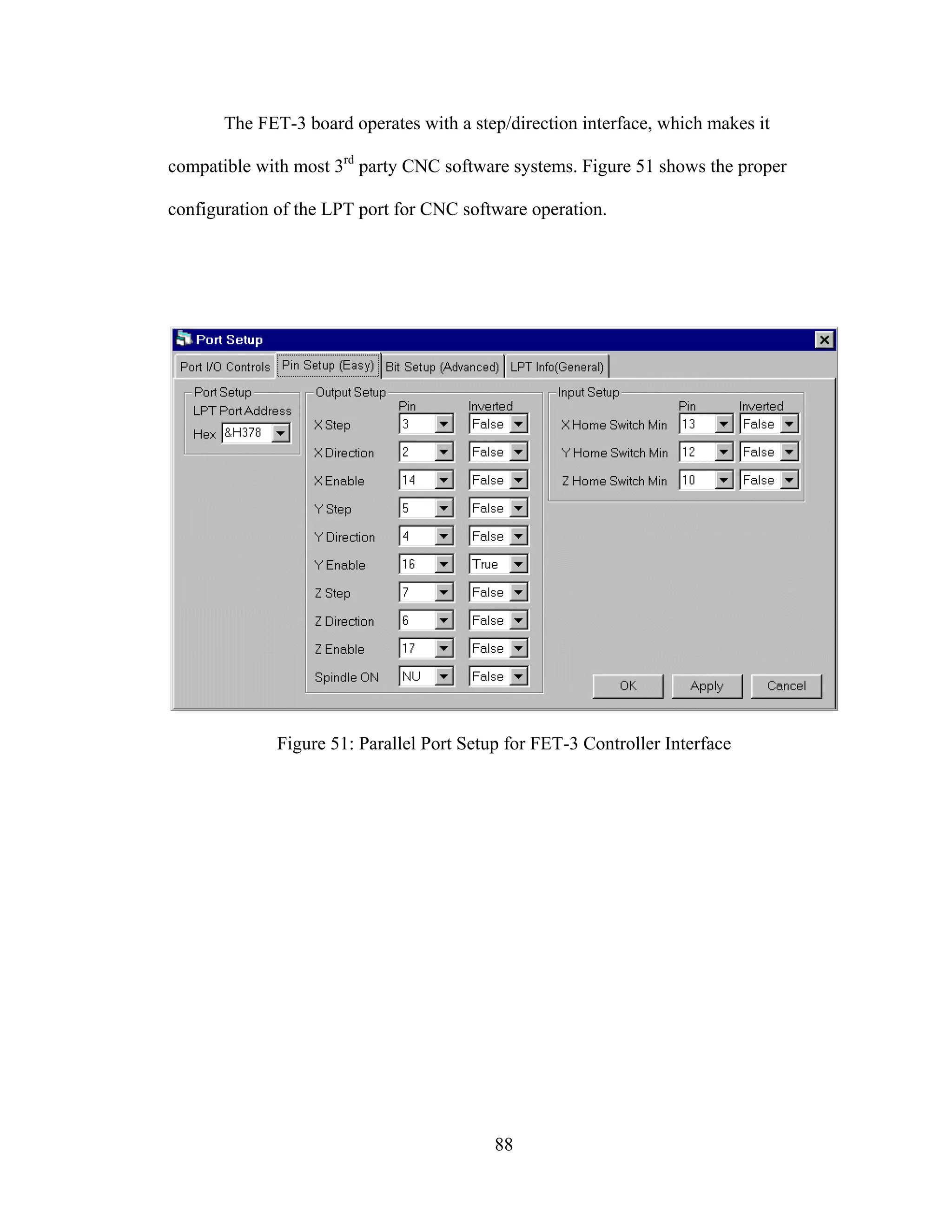
• Step and Direction Interface (compatible with 3rd party software)
• Dip Switch Mode Selection for each axis - Wave drive, Hi-Torque, Half Step
• 3 Switch Inputs for Limit Detection
• Connects to Parallel Port with Standard DB-25 Cable
• Optional Separate Power Supply Input for Z axis
• 50 VDC Maximum Motor Supply Voltage](https://image.slidesharecdn.com/designcontrolandimplementationofathreelink-190121102715/75/Design-control-and-implementation-of-a-three-link-94-2048.jpg)
![92
The control board uses the parallel port logic described above to power the
stepper motors. Figure 54 shows the pin out of the connector and table 8 describes the
function of the pins.
Figure 54: Standard Parallel Port Pinout [2]
Table 8: SP-3/FET-3 Stepper Parallel Port Pin Assignments (DB25 Connector)
Pin [Bit] Address I/O Function
2- [D0] bs OUTPUT X axis direction
3- [D1] bs OUTPUT X axis step
4- [D2] bs OUTPUT Y axis direction
5- [D3] bs OUTPUT Y axis step
6- [D4] bs OUTPUT Z axis direction
7- [D5] bs OUTPUT Z axis step
8- [D6] bs OUTPUT Aux Out (d6)
9- [D7] bs OUTPUT Aux Out (d7)
10- [S6] bs+1 OUTPUT Z switch detect
12- [S5] bs+1 OUTPUT Y switch detect
13- [S4] bs+1 OUTPUT X switch detect
14- [C1] bs+2 OUTPUT X axis *Enable (active LO)
16- [C2] bs+2 OUTPUT Y axis *Enable (active LO)
17- [C3] bs+2 OUTPUT Z axis *Enable (active LO)
18- Ground
25- Ground](https://image.slidesharecdn.com/designcontrolandimplementationofathreelink-190121102715/75/Design-control-and-implementation-of-a-three-link-100-2048.jpg)
![101
BIBLIOGRAPHY
References:
[4] McKerrow, Phillip John: Introduction to Robotics, Addison-Wesley Publishing,
1991
[1] Shelton, Bob: “Types of Robots. NASA ROVer Ranch Website.” 2003.
<http://prime.jsc.nasa.gov/ROV/types.html>
[2] Beauchemin, George A.: “Stepper Motor Technical Note: Microstepping Myths
and Realities.” 2003, MicroMo Electronics, Inc. <http://www.micro-drives.com>
[3] Baldor Electric Company: “Servo Control Facts: A Handbook Explaining the
Basics of Motion” 1994, Baldor Electric Company.
<http://www.baldor.com/pdf/manuals/1205-394.pdf>
[5] New Japan Radio Company: “Drive Circuit Basics.” New Japan Radio Company
Ltd. <www.njr.co.jp/pdf/ee/ee05002.pdf>
[6] Chernousko, Falex L.: Manipulation Robots, CRC Press, 1993
[7] Peacock, Craig: “Interfacing the Standard Parallel Port.” 2005 Beyond Logic.
<http://www.beyondlogic.org/spp/parallel.htm>
[8] Tyson, Jeff: “How Parallel Ports Work.” 2005 How Stuff Works.
<http://computer.howstuffworks.com/parallel-port1.htm>
[9] Kelly, Alonzo: “Introduction to Mobile Robots.” 1996, Carnegie Mellon
University <https://www.andrew.cmu.edu/course/16-761/Documentation/>
[10] Schwartz, Jacob T, Sharir, Micha: “On the Piano Movers’ Problem.” 1981, New
York University, Dept. of Computer Science.
[11] Amato, Nancy: “A Brief Introduction: The Motion Planning Problem,
Configuration Space, Basic Path Planning Methods.” 2004, University of Padova.
<http://parasol.tamu.edu/~amato/Courses/padova04/lectures/L1.intro.pdf>](https://image.slidesharecdn.com/designcontrolandimplementationofathreelink-190121102715/75/Design-control-and-implementation-of-a-three-link-109-2048.jpg)
![102
[12] Duindam, Vincent, Stramigioli, Stefano: “Passive Asymptotic Curve Tracking.”
IFAC Workshop on Lagr. and Hamilt. Methods for Nonlinear Control, pages 229
– 234 April 2003
[13] Vincent Duindam, Stefano Stramigioli: “Port-Based Asymptotic Curve Tracking
for Mechanical Systems.” European Journal of Control, Volume 10(5), pages 411
– 420 December 2004
[14] Jing Lin, Hui-Tang Chen, Ping Jiang, Yue-Juan Wang, Peng-Yung Woo. Curve
Tracking and Reproduction by a Robot with a Vision System
[15] Laidman Russell. “Interfacing the FET-3 Stepper Controller”. 2000,StepperWorld
<http://www.stepperworld.com>
[16] Benson, Harris. University Physics. 1996 Rand McNally NewYork ISBN 0-471-
00689-0
[17] Brown, Ward. Brushless DC Motor Control Made Easy. 2002, Microchip
Technology Inc.
[18] Laidman Russell. “Unipolar Stepper Motors and Control”. 1999 StepperWorld
<http://www.stepperworld.com>
[19] Malcom, Douglas R. Robotics, an Introduction. 1988. Delmar Publishers. Albany,
New York
[20] Advanced Micro Systems: “Stepper Motor System Basics.” 2008, Advanced
Micro Systems. <http://www.ams2000.com/stepping101.html>
[21] Jones, Douglas W. “Control of stepping motors,” 1998, University of Iowa.
<http://www.cs.uiowa.edu/~jones/step/>
[22] Liu, Yuhang. Design and Control Simulation of a Robot Arm. Master’s Thesis
2004, University of Akron.
[23] Lin Engineering. Data sheets 1.8° NEMA size 17 standard step motor.
[24] Lin Engineering. Data sheets 1.8° NEMA size 23 standard step motor.
[25] Lin Engineering. Data sheets Wiring diagram 6 lead standard step motor.
[26] Laidman, Russell. Data sheet FET-3 stepper motor controller. 2000,
StepperWorld <http://www.stepperworld.com>](https://image.slidesharecdn.com/designcontrolandimplementationofathreelink-190121102715/75/Design-control-and-implementation-of-a-three-link-110-2048.jpg)


![120
I2*sinecosine12+m2*l1*lc2*sine2)*(v^2)+m2*lc2*cosine12;
angle1=theta1(1);
angle2=theta2(1);
tt2=[];
%Find solution
for i=1:length(theta1)
for j=1:length(theta2)
sine12=sin(theta1(i)+theta2(j));
cosine12=cos(theta1(i)+theta2(j));
sinecosine12=sine12*cosine12;
cosine1=cos(theta1(i));
cosine2=cos(theta2(j));
sine2=sin(theta2(j));
torque2=(m2*l1*lc2*cosine2+2*(m2*lc2^2+I2))*a+...
(m2*(l1*lc2*cosine1*sine12+lc2^2*sinecosine12)+...
I2*sinecosine12+m2*l1*lc2*sine2)*(v^2)+m2*lc2*cosine12;
tt2=[tt2 torque2];
if abs(torque2)>abs(torque);
torque=torque2;
angle1=theta1(i);
angle2=theta2(j);
end
end
end
%Display max torque in lbs. and oz.
torque
torque*16
%Display and of link 1 and link 2 where the maximum torque occurs
angle1*180/pi
angle2*180/pi
%Plot the torque curve
k=1:(70+41)*(90+81);
plot(k,tt2)
xlabel('Time t')
ylabel('Torque T_2')](https://image.slidesharecdn.com/designcontrolandimplementationofathreelink-190121102715/75/Design-control-and-implementation-of-a-three-link-128-2048.jpg)

![122
sinecosine12=sine12*cosine12;
sine1cosine1=sine1*cosine1;
sine1cosine12=sine1*cosine12;
cosine1sine12=cosine1*sine12;
%Torque?
torque=(m1*lc1^2+I1+m2*l1^2+2*m2*l1*lc2*cosine2+m2*lc2^2+I2)*a+...
(m2*l1*lc2*cosine2+m2*lc2^2+I2)*a+...
((m1*lc1^2+I1)*sine1cosine1+m2*(l1^2*sine1cosine1+l1*lc2*(sine1cosine12+cosine1si
ne12)+lc2^2*sinecosine12)+...
m1*lc1*cosine1+m2*(l1*cosine1+lc2*cosine12));
angle1=theta1(1);
angle2=theta2(1);
tt1=[];
%Find solution
for i=1:length(theta1)
for j=1:length(theta2)
sine12=sin(theta1(i)+theta2(j));
cosine12=cos(theta1(i)+theta2(j));
sinecosine12=sine12*cosine12;
cosine1=cos(theta1(i));
cosine2=cos(theta2(j));
sine1=sin(theta1(1));
sine2=sin(theta2(j));
sine1cosine1=sine1*cosine1;
sine1cosine12=sine1*cosine12;
cosine1sine12=cosine1*sine12;
torque1=(m1*lc1^2+I1+m2*l1^2+2*m2*l1*lc2*cosine2+m2*lc2^2+I2)*a+...
(m2*l1*lc2*cosine2+m2*lc2^2+I2)*a+...
((m1*lc1^2+I1)*sine1cosine1+m2*(l1^2*sine1cosine1+l1*lc2*(sine1cosine12+c
osine1sine12)+lc2^2*sinecosine12)+...
m1*lc1*cosine1+m2*(l1*cosine1+lc2*cosine12));
tt1=[tt1 torque1];
if abs(torque1)>abs(torque);
torque=torque1;
angle1=theta1(i);
angle2=theta2(j);
end
end
end](https://image.slidesharecdn.com/designcontrolandimplementationofathreelink-190121102715/75/Design-control-and-implementation-of-a-three-link-130-2048.jpg)

![125
cosine12=cos(theta1(1)+theta2(1));
sinecosine12=sine12*cosine12;
sine1cosine1=sine1*cosine1;
sine1cosine12=sine1*cosine12;
cosine1cosine12=cosine1*cosine12;
cosine1sine12=cosine1*sine12;
%Torque?
torque=(I0+(m1*lc1^2+I1)*cosine1^2+m2*l1*(l1*cosine1^2+2*lc2*cosine1cosine12)+(
m2*lc2^2+I2)*cosine12^2)...
*a-
2*((m1*lc1^2+I1)*sine1cosine1+m2*l1*(l1*sine1cosine1+lc2*sine1cosine12+lc2*cosin
e1sine12)+(m2*lc2^2+I2)*sinecosine12)...
*v^2-2*(m2*l1*lc2*cosine1sine12+(m2*lc2^2+I2)*sinecosine12)*v^2-
2*(m2*l1*lc2*cosine1sine12+(m2*lc2^2+I2)*sinecosine12)*v^2;
angle1=theta1(1);
angle2=theta2(1);
tt0=[];
%Find solution
for i=1:length(theta1)
for j=1:length(theta2)
sine12=sin(theta1(i)+theta2(j));
cosine12=cos(theta1(i)+theta2(j));
sinecosine12=sine12*cosine12;
cosine1=cos(theta1(i));
%cosine2=cos(theta2(j));
sine1=sin(theta1(1));
%sine2=sin(theta2(j));
sine1cosine1=sine1*cosine1;
sine1cosine12=sine1*cosine12;
cosine1sine12=cosine1*sine12;
torque0=(I0+(m1*lc1^2+I1)*cosine1^2+m2*l1*(l1*cosine1^2+2*lc2*cosine1cos
ine12)+(m2*lc2^2+I2)*cosine12^2)...
*a-
2*((m1*lc1^2+I1)*sine1cosine1+m2*l1*(l1*sine1cosine1+lc2*sine1cosine12+lc2*cosin
e1sine12)+(m2*lc2^2+I2)*sinecosine12)...
*v^2-2*(m2*l1*lc2*cosine1sine12+(m2*lc2^2+I2)*sinecosine12)*v^2-
2*(m2*l1*lc2*cosine1sine12+(m2*lc2^2+I2)*sinecosine12)*v^2;
tt0=[tt0 torque0];
if abs(torque0)>abs(torque);
torque=torque0;
angle1=theta1(i);](https://image.slidesharecdn.com/designcontrolandimplementationofathreelink-190121102715/75/Design-control-and-implementation-of-a-three-link-133-2048.jpg)

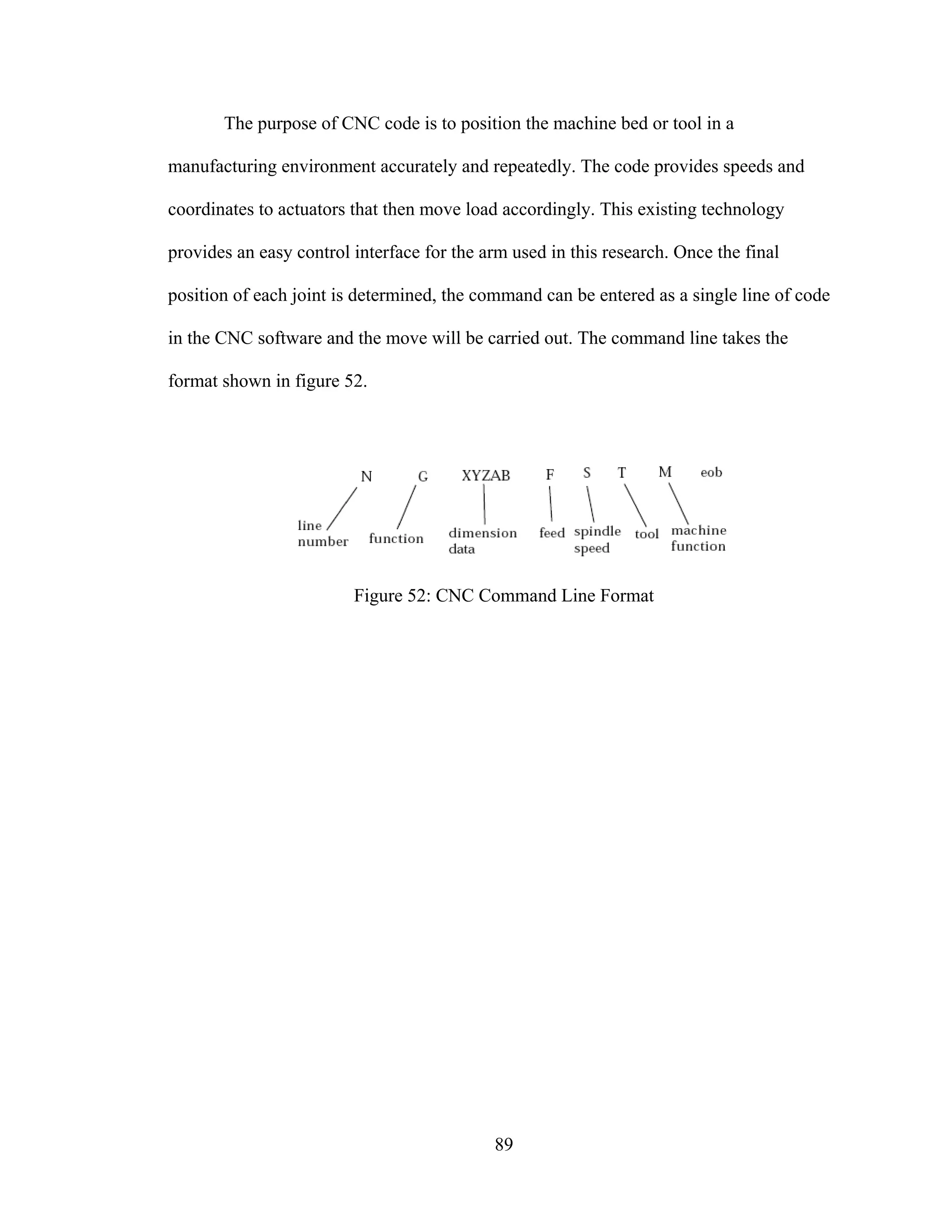
This document presents a thesis on the design, control, and implementation of a three link articulated robot arm. It includes an introduction and outlines chapters on reviewing robotic systems, robot dynamics, and the design of the robot arm. The chapters will cover actuators, controllers, coordinate transformations, dynamic behavior modeling, and the detailed design of the constructed robot arm including motor selection, static and dynamic analysis, and assembly procedures.


![Vibe Coding vs. Spec-Driven Development [Free Meetup]](https://cdn.slidesharecdn.com/ss_thumbnails/vibecodingvsspecdrivendevelopment-251209105622-43f455e7-thumbnail.jpg?width=640&height=640&fit=bounds)


