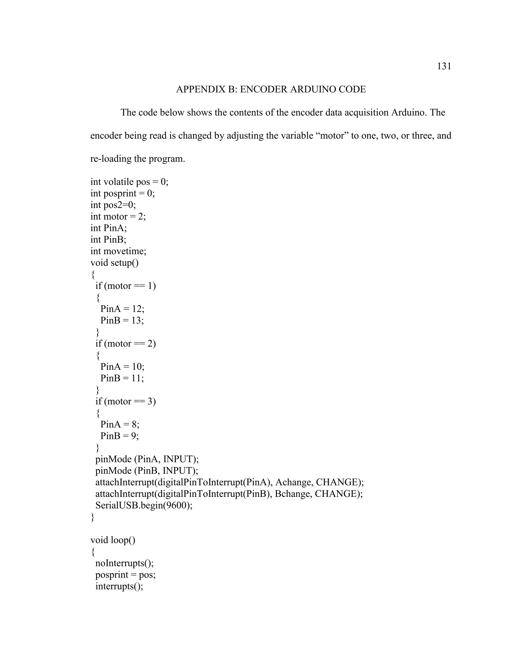
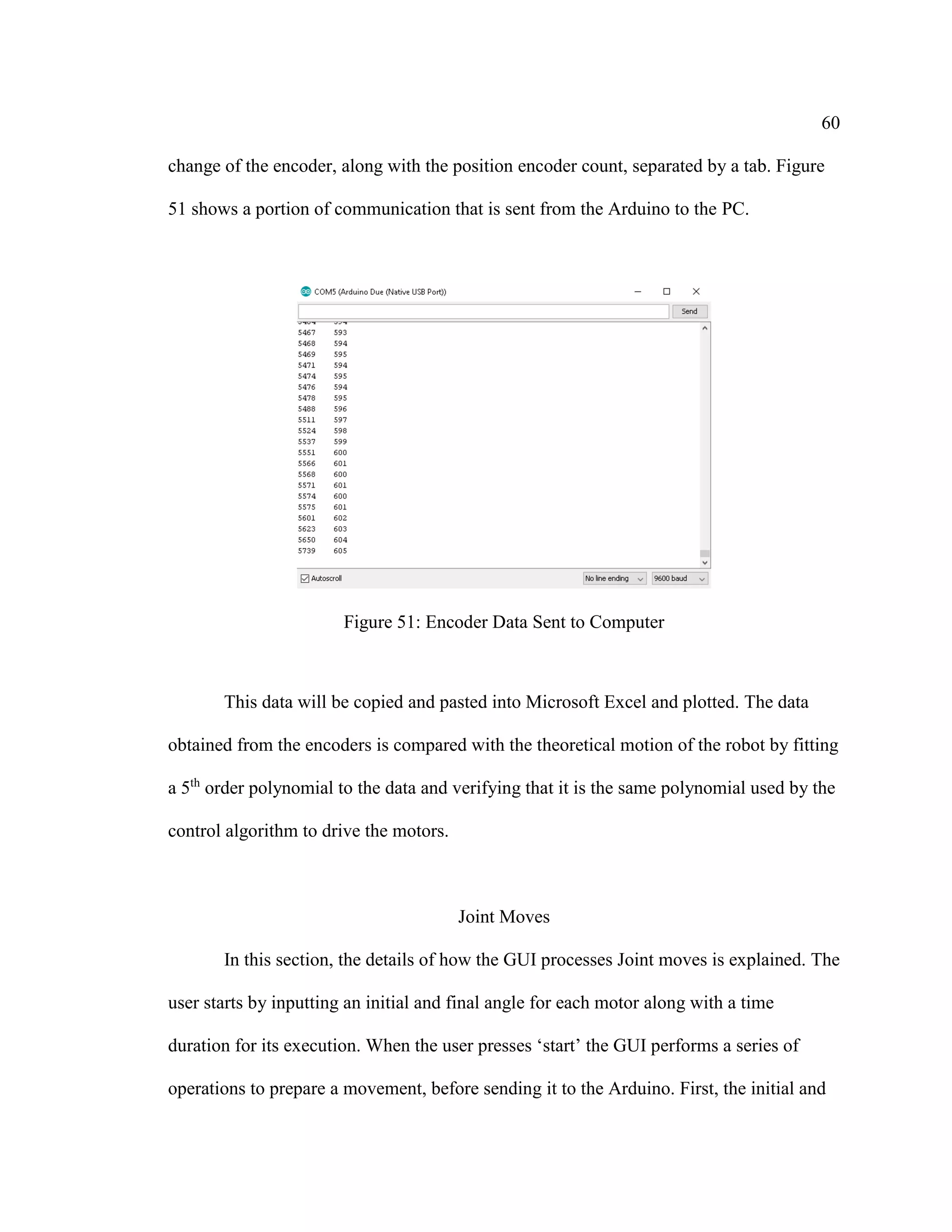
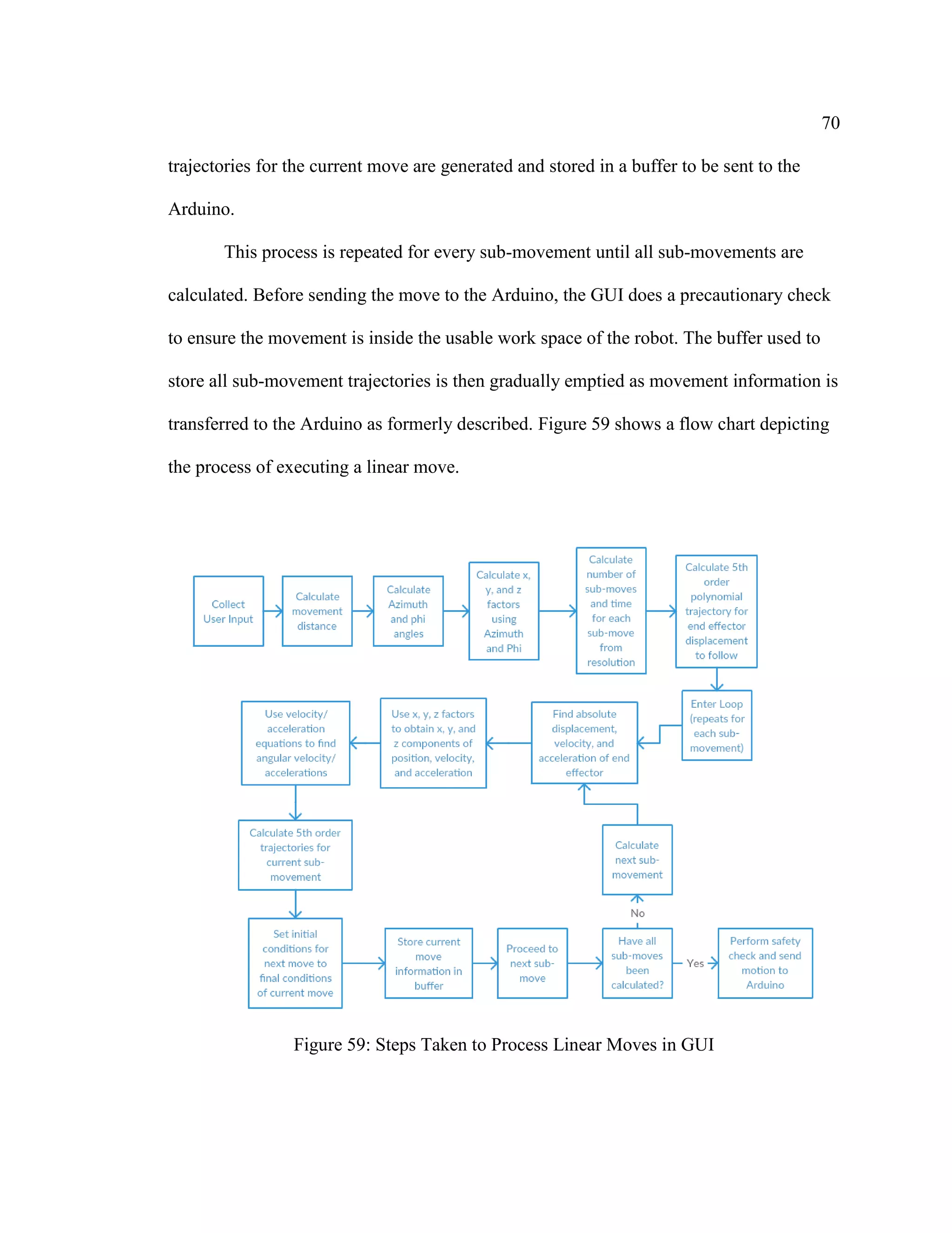
This thesis presents the design, construction, control, and analysis of a linear input Delta robot. The robot was designed and built to improve upon previous Delta robot designs for 3D printing applications. A novel method of controlling the robot using 5th order polynomial trajectories was developed to prevent jerk spikes that occur with traditional control methods. Experimental analysis was performed to characterize the robot's velocity, accuracy, and motion capabilities both theoretically and experimentally. The results demonstrate the robot functions as intended and the control method successfully eliminates jerk spikes.

1. Design, Construction, Control, and Analysis of Linear Delta Robot
A thesis presented to
the faculty of
the Russ College of Engineering and Technology of Ohio University
In partial fulfillment
of the requirements for the degree
Master of Science
Joseph Q. Oberhauser
April 2016
© 2016 Joseph Q. Oberhauser. All Rights Reserved.

2. 2
This thesis titled
Design, Construction, Control, and Analysis of Linear Delta Robot
by
JOSEPH Q. OBERHAUSER
has been approved for
the Department of Mechanical Engineering
and the Russ College of Engineering and Technology by
Robert L. Williams II
Professor of Mechanical Engineering
Dennis Irwin
Dean, Russ College of Engineering and Technology

3. 3
ABSTRACT
OBERHAUSER, JOSEPH Q., M.S., April 2016, Mechanical Engineering
Design, Construction, Control, and Analysis of Linear Delta Robot
Director of Thesis: Robert L. Williams II
Linear Delta Robots are a technology that are primarily used for 3D printing. The
technology is still in its infancy and there are many improvements which can be made.
This thesis involves the design and construction of a new linear Delta Robot design with
several advantages over previous models. This thesis also describes a new method of
controlling a linear Delta Robot via 5th
order polynomial trajectory generation. This new
method of control is an improvement over traditional methods because it prevents the
occurrence of infinite jerk spikes, a problem that occurs with traditional robot and 3D
printer control. The physical capabilities of the robot are obtained and reported
theoretically and experimentally.

4. 4
ACKNOWLEDGMENTS
I would like to express my sincere gratitude to my advisor Dr. Robert L Williams
II for his continued support, knowledge, and patience. His guidance was the driving force
behind me attending graduate school and obtaining my masters’ degree.
I would also like to thank my wife for her love, support, and understanding for all
of the long hours I spent dedicated to my schooling and research.

5. 5
TABLE OF CONTENTS
Page
Abstract............................................................................................................................... 3
Acknowledgments............................................................................................................... 4
List of Figures..................................................................................................................... 7
Chapter 1- Introduction and Literature Review................................................................ 11
Literature Review ......................................................................................................... 12
Parallel vs Serial Robots............................................................................................... 13
Current Methods of Control.......................................................................................... 17
Current 3D Printer and Home CNC/Robot Control...................................................... 20
Current Delta Robots .................................................................................................... 21
Thesis Purpose.............................................................................................................. 23
Objectives and Problem Statement............................................................................... 25
Objective 1- Design and Construction of Linear Input Delta Robot ........................ 25
Objective 2- Achieve Control via 5th
Order Polynomial Trajectories ...................... 25
Objective 3- Analyze Robot Experimentally and Theoretically............................... 26
Chapter 2- Methods........................................................................................................... 27
Robot Design ................................................................................................................ 27
Unique Design Choices ................................................................................................ 29
Control of the Robot ..................................................................................................... 45
Linear Delta Robot Kinematics .................................................................................... 49
5th
Order Polynomial Trajectory Generation ................................................................ 52
GUI Software................................................................................................................ 53
Serial Communication .................................................................................................. 56
Joint Moves................................................................................................................... 60
Cartesian Moves ........................................................................................................... 62
Velocity and Acceleration Equations ........................................................................... 62
Linear and Circular Moves ........................................................................................... 65
Linear Moves ............................................................................................................ 68
Circular Moves.......................................................................................................... 71

6. 6
Arduino Motion Control............................................................................................... 75
Motion Control Algorithm........................................................................................ 75
Zeroing Protocol ....................................................................................................... 77
Analysis ........................................................................................................................ 78
Velocity Analysis...................................................................................................... 79
Motion Analysis........................................................................................................ 81
Accuracy Analysis .................................................................................................... 81
Chapter 3- Results............................................................................................................. 87
Velocity Analysis Results............................................................................................. 87
Accuracy Analysis Results ........................................................................................... 89
Motion Analysis Results............................................................................................... 93
Cartesian/Joint Motion Analysis Results.................................................................. 94
Circular/Linear Move Motion Analysis.................................................................... 98
Circular Move Plots ................................................................................................ 100
Linear Move Plots................................................................................................... 103
Chapter 4- Discussion..................................................................................................... 106
GUI Discussion........................................................................................................... 106
Motion Control Algorithm Discussion ....................................................................... 107
Robot Design Discussion............................................................................................ 109
Robot Analysis Discussion ......................................................................................... 111
Chapter 5- Conclusion .................................................................................................... 113
Unique Contributions.................................................................................................. 113
Future Work................................................................................................................ 114
References....................................................................................................................... 115
Appendix A: Motion Control Arduino Code.................................................................. 120
Appendix B: Encoder Arduino Code.............................................................................. 131
Appendix C: Encoder Wiring Diagram .......................................................................... 134
Appendix D: Download Links (DropBox) ..................................................................... 135

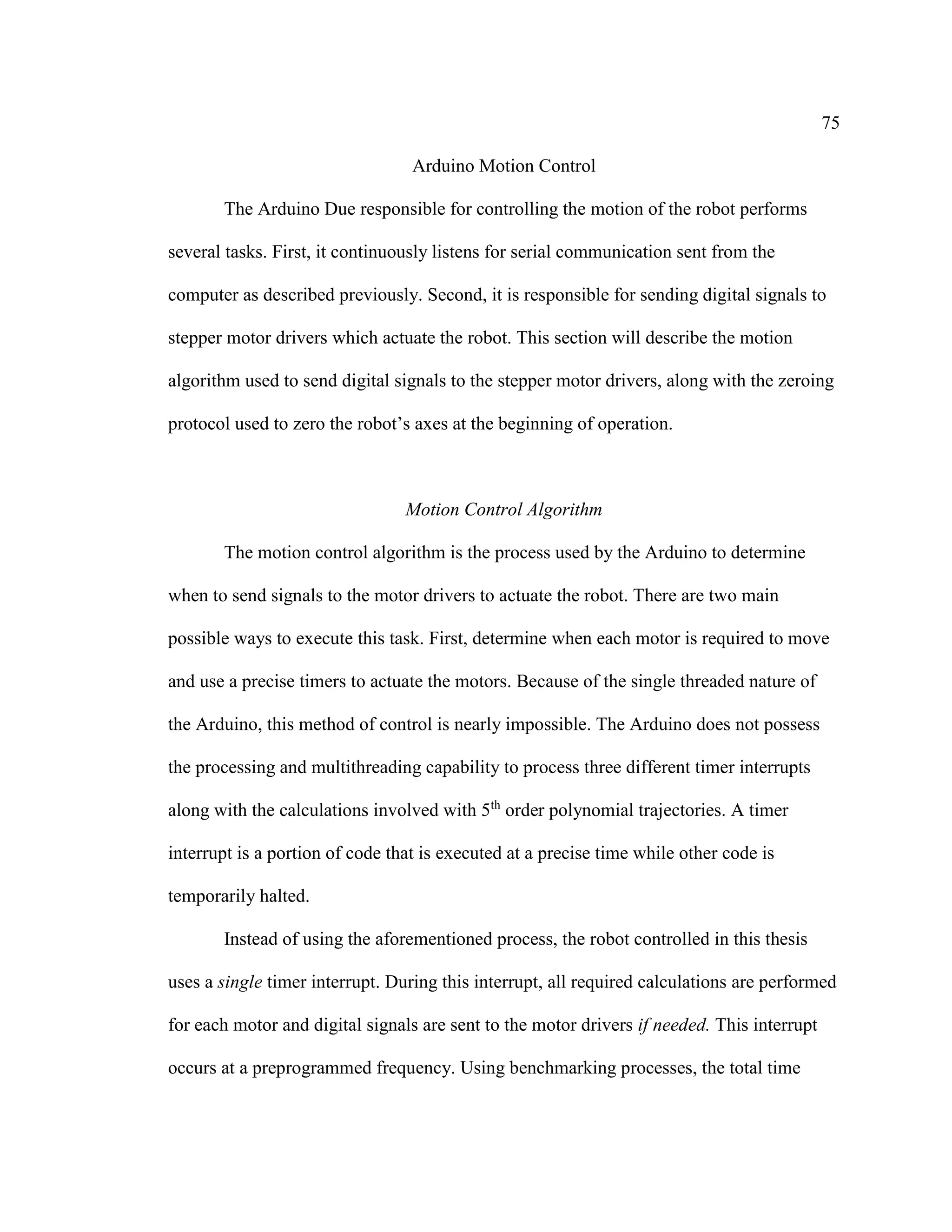
7. 7
LIST OF FIGURES
Page
Figure 1: Clavel’s Delta Robot [8].................................................................................... 12
Figure 2: Linear Input Delta Robot [6]............................................................................. 13
Figure 3: Fanuc Robotic Arm [9]...................................................................................... 14
Figure 4: Traditional Cartesian 3D Printer ....................................................................... 15
Figure 5: Serial and Parallel Robot Comparison [3]......................................................... 16
Figure 6: Trapezoidal Velocity Profile [12]...................................................................... 17
Figure 7: 3rd
Order Polynomial Trajectory Profile [10].................................................... 18
Figure 8: Delta Robot Information ................................................................................... 21
Figure 9: A- Deltamaker 3D Printer[40] B- ORION 3D Printer[23] C- Kossel Mini 3D
Printer [24]........................................................................................................................ 22
Figure 10: A- Deltaprintr 3D Printer [25] B- Fanuc M-1iA Delta Robot [26]................. 22
Figure 11: Final Robot Design.......................................................................................... 24
Figure 12: Motions Executable by Robot. ........................................................................ 26
Figure 13: Timing Belt Driving Linear Motion Along Hardened Rods ........................... 28
Figure 14: NEMA 17 Stepper Motor................................................................................ 28
Figure 15: Two Parallel Links Connecting Each Carriage to End Effector ..................... 28
Figure 16: Deltamaker 3D printer (Hexagonal Frame) [40]............................................. 29
Figure 17: Top View of Robot, Showing the Hexagonal Shape of the Frame. ................ 30
Figure 18: A- Deltaprintr Linear Inputs Riding Directly on Vertical Supports [25] B-
Rod End Supports used to Secure Hardened Rods ........................................................... 31
Figure 19: A- Plexiglas Reinforcements Used to Stiffen Frame B- Electronic Hardware
Mounted to Plexiglas Sheet .............................................................................................. 32
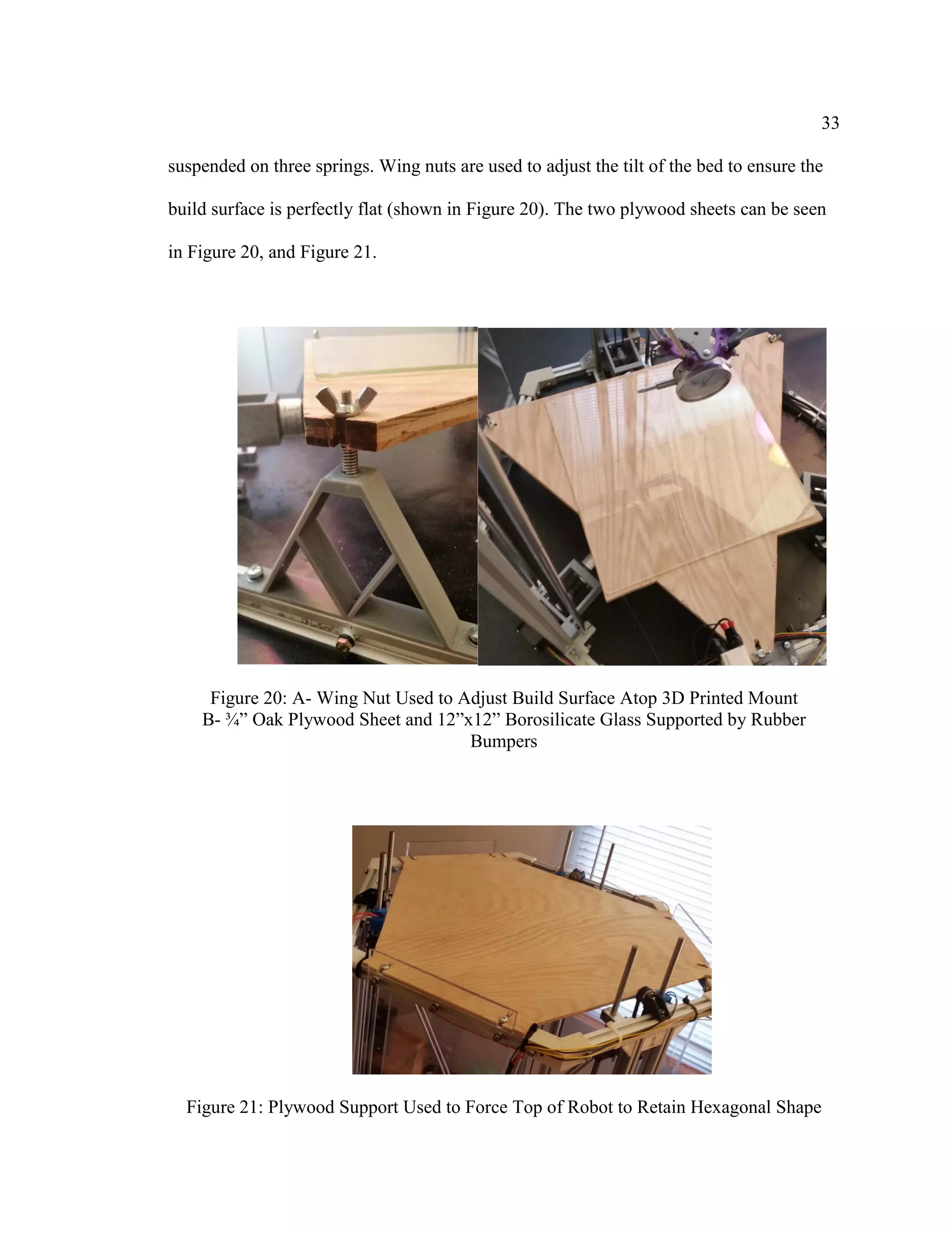
Figure 20: A- Wing Nut Used to Adjust Build Surface Atop 3D Printed Mount B- ¾”
Oak Plywood Sheet and 12”x12” Borosilicate Glass Supported by Rubber Bumpers..... 33
Figure 21: Plywood Support Used to Force Top of Robot to Retain Hexagonal Shape .. 33
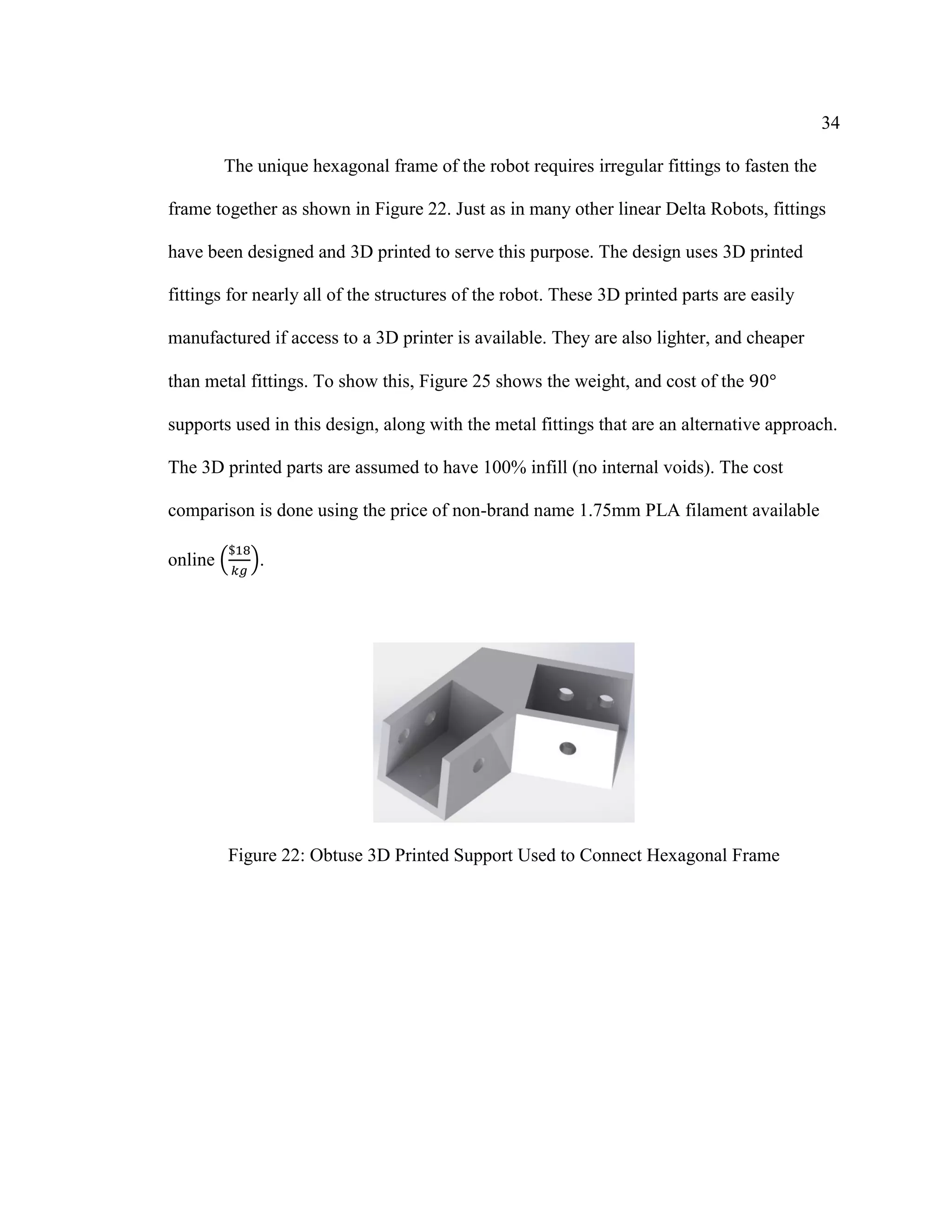
Figure 22: Obtuse 3D Printed Support Used to Connect Hexagonal Frame .................... 34
Figure 23: 3D Printed Fitting............................................................................................ 35

8. 8
Figure 24: Steel Fitting ..................................................................................................... 35
Figure 25: Mass and Cost Comparison of 3D Printed (PLA) and Machined Metal 90°
Fittings (McMaster Carr).................................................................................................. 35
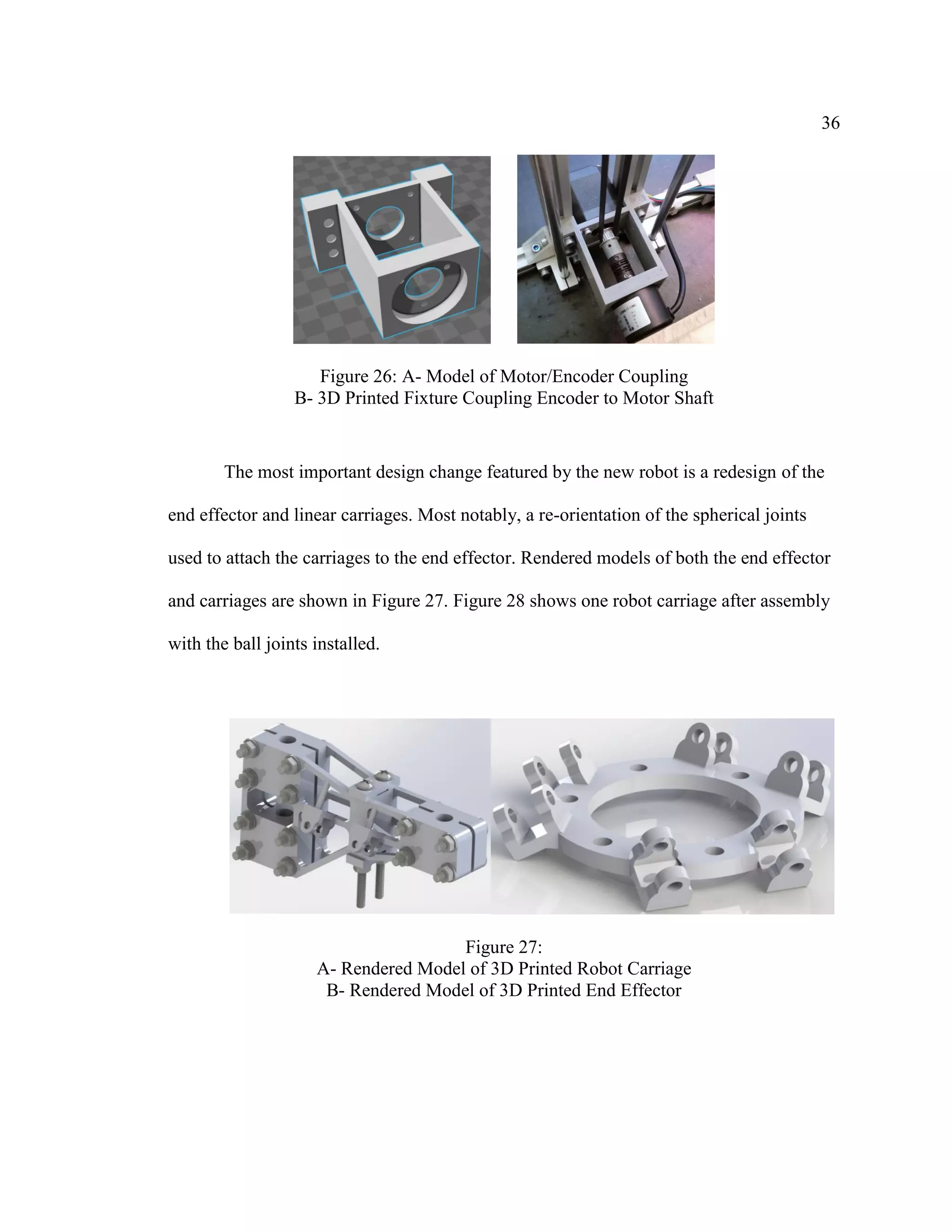
Figure 26: A- Model of Motor/Encoder Coupling B- 3D Printed Fixture Coupling
Encoder to Motor Shaft..................................................................................................... 36
Figure 27: A- Rendered Model of 3D Printed Robot Carriage B- Rendered Model of 3D
Printed End Effector ......................................................................................................... 36
Figure 28: 3D Printed Robot Carriage with Ball Joints.................................................... 37
Figure 29: A- 3D Printed Universal Joints [28] B- Magnetic Ball Joints [29]................. 37
Figure 30: Traxxas Rod End Ball Joints........................................................................... 38
Figure 31: A- Restrictive Orientation of Rod End Ball Joints [30] B- New Orientation of
Rod End Ball Joints .......................................................................................................... 39
Figure 32: A- Joint Limitation of End Effector (Side View) B- Joint Limitation of
Carriage (Top View)......................................................................................................... 39
Figure 33: A- Joint Limit of End Effector (Top View) B- Joint Limit of Carriage (Side
View)................................................................................................................................. 40
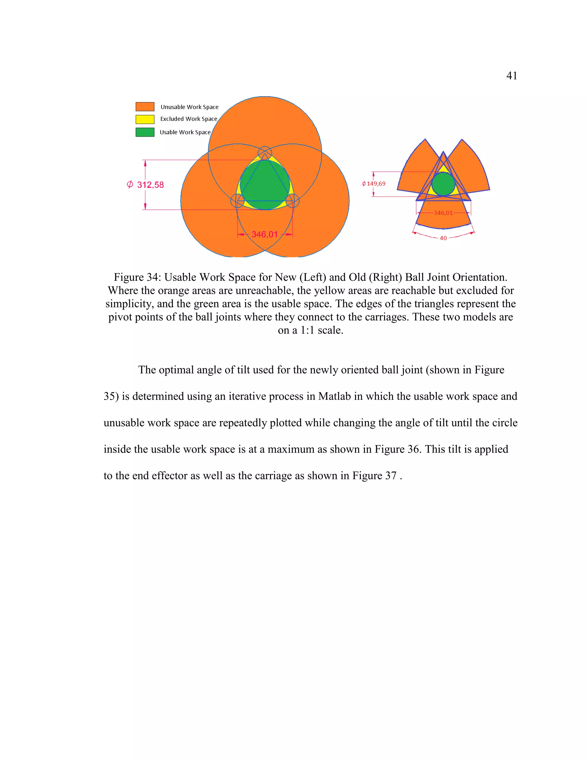
Figure 34: Usable Work Space for New (Left) and Old (Right) Ball Joint Orientation... 41
Figure 35: Optimal Angle of Tilt for New Ball Joint Orientation (60°)........................... 42
Figure 36: Matlab Plot Used to Iteratively Determine the Optimal Ball Joint Tilt to
Maximize Usable Work Area. .......................................................................................... 42
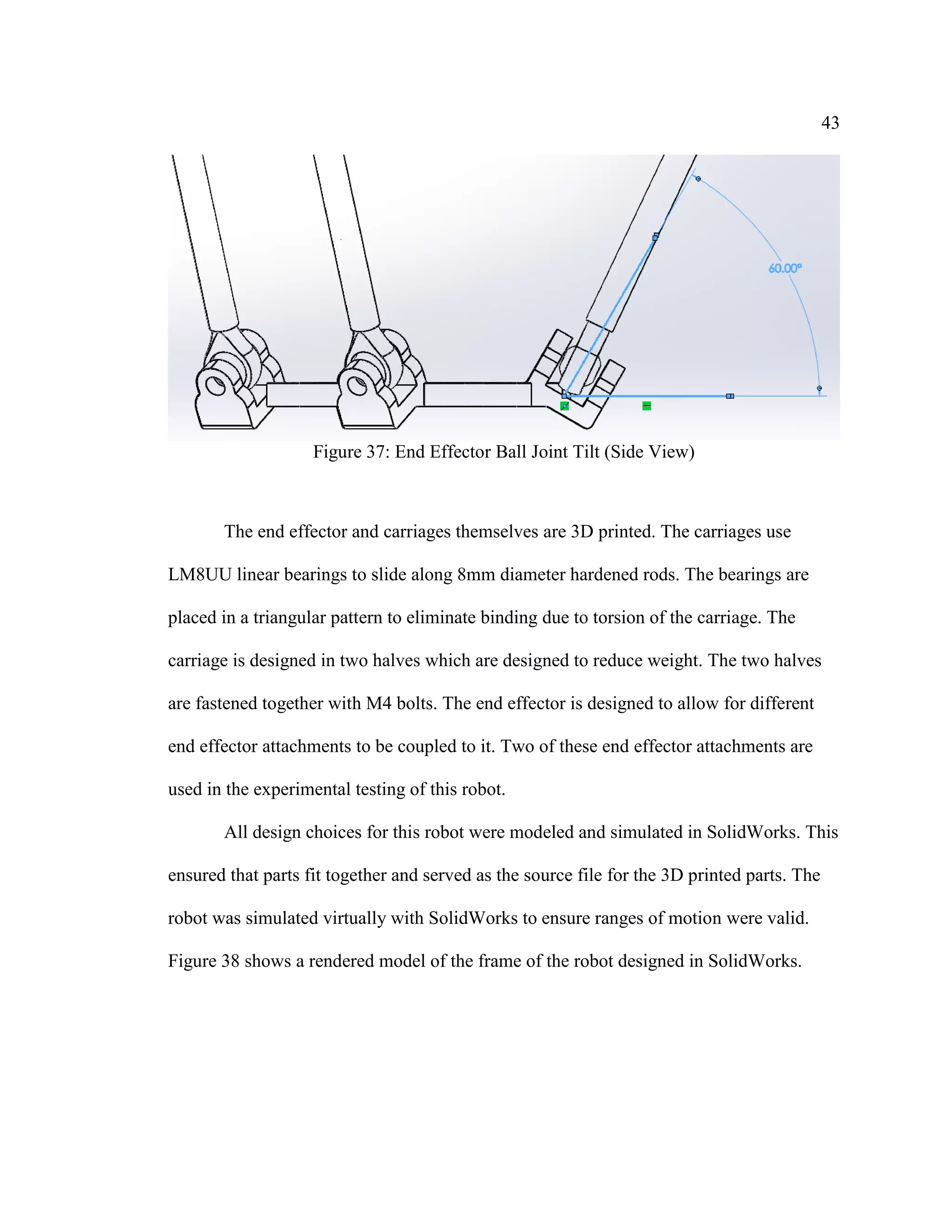
Figure 37: End Effector Ball Joint Tilt (Side View)......................................................... 43
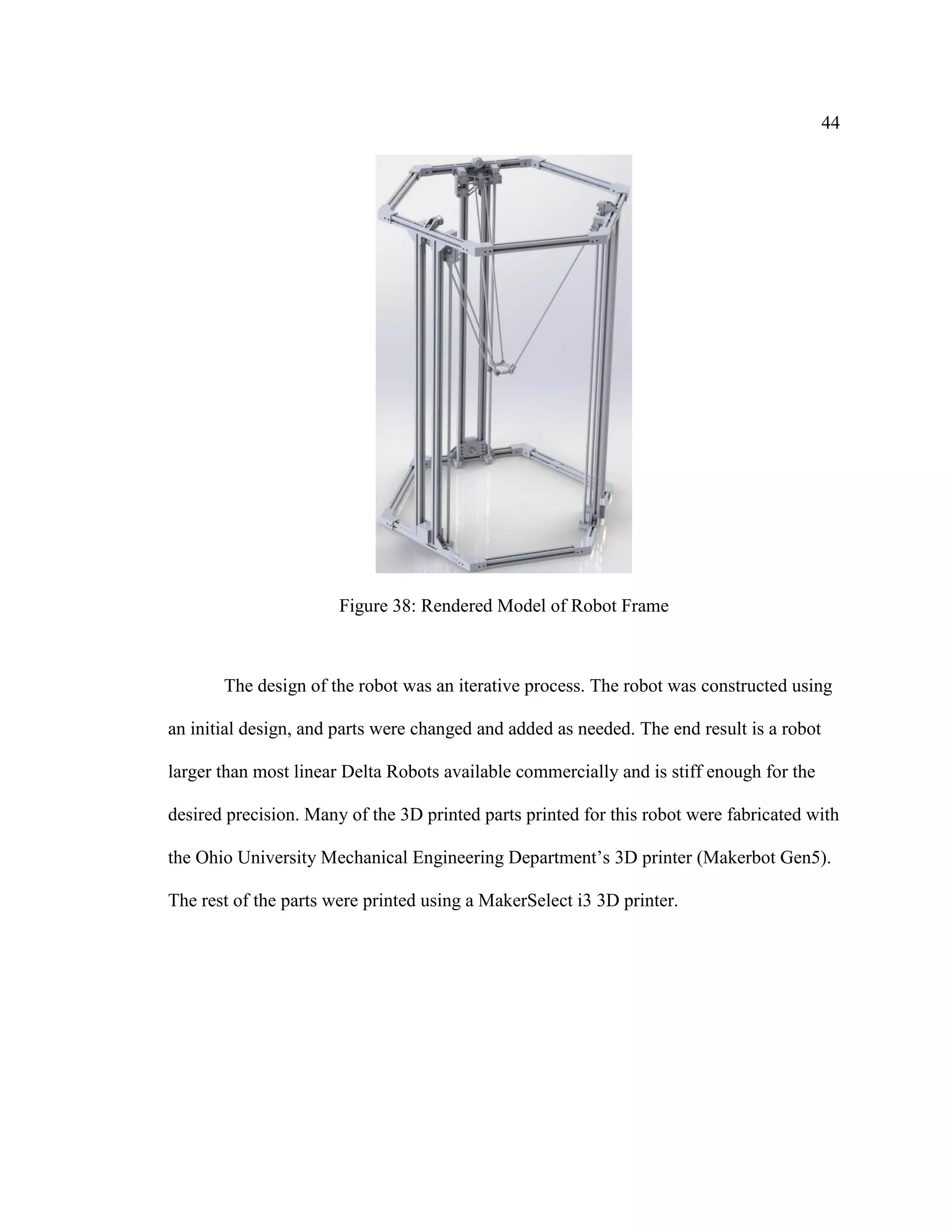
Figure 38: Rendered Model of Robot Frame.................................................................... 44
Figure 39: Pololu A4988 Stepper Motor Driver [32] ....................................................... 46
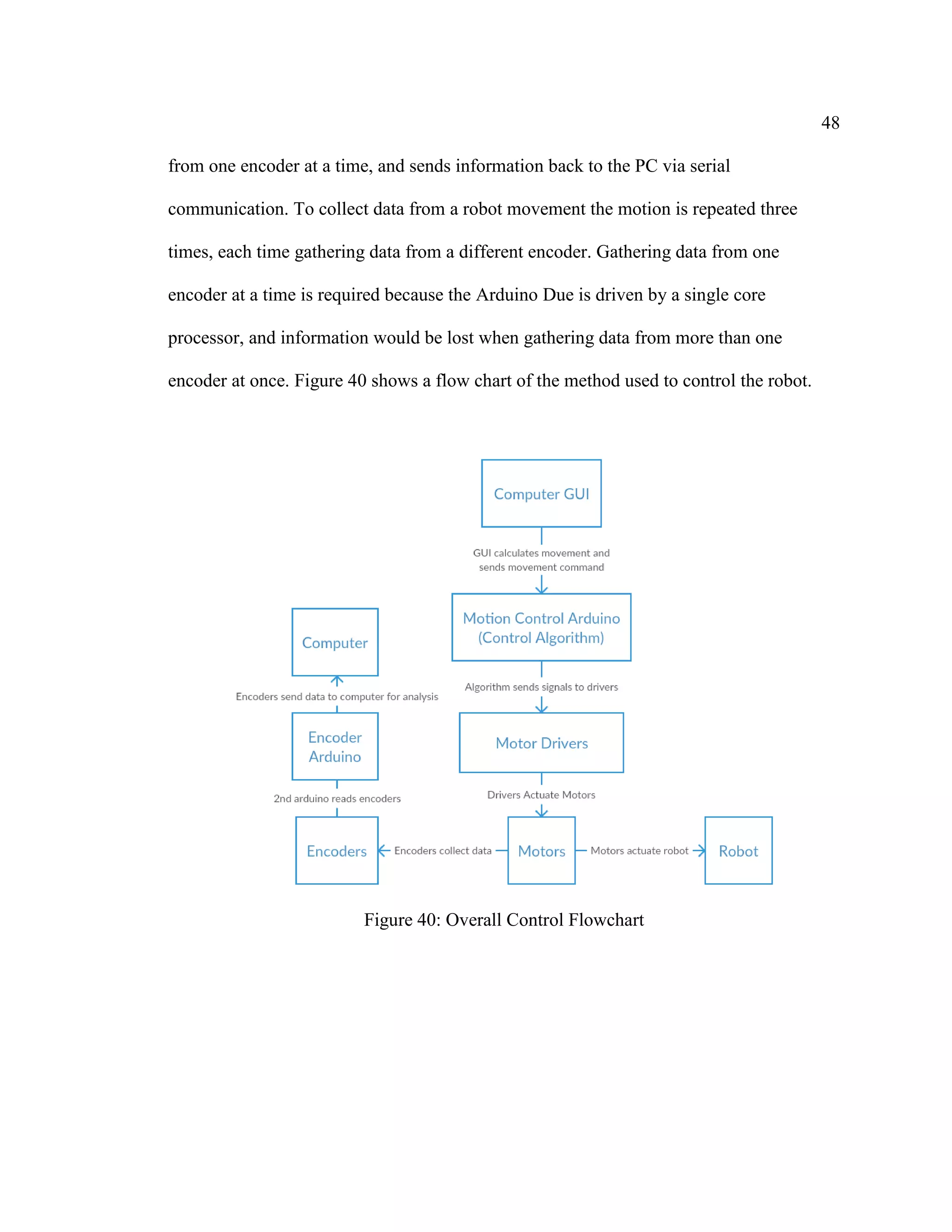
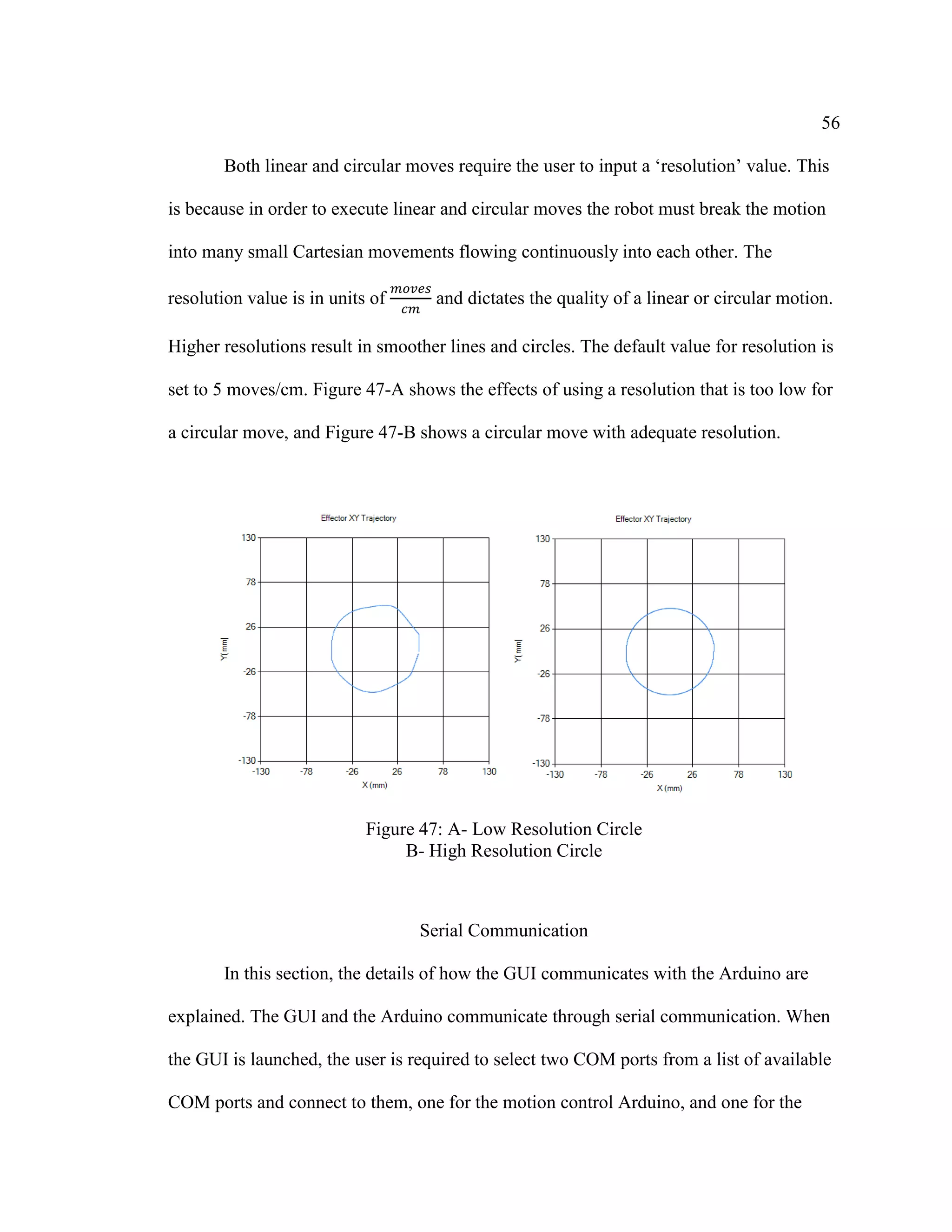
Figure 40: Overall Control Flowchart............................................................................... 48
Figure 41: 3D View of Linear Delta Robot Coefficients [5]............................................ 50
Figure 42: A- Top View of Robot Frame [5] B- Top View of Robot End Effector [5] ... 50
Figure 43: Essential Variables used in linear Delta Robot IPK/FPK [5].......................... 52
Figure 44: Circular Check [36]......................................................................................... 52
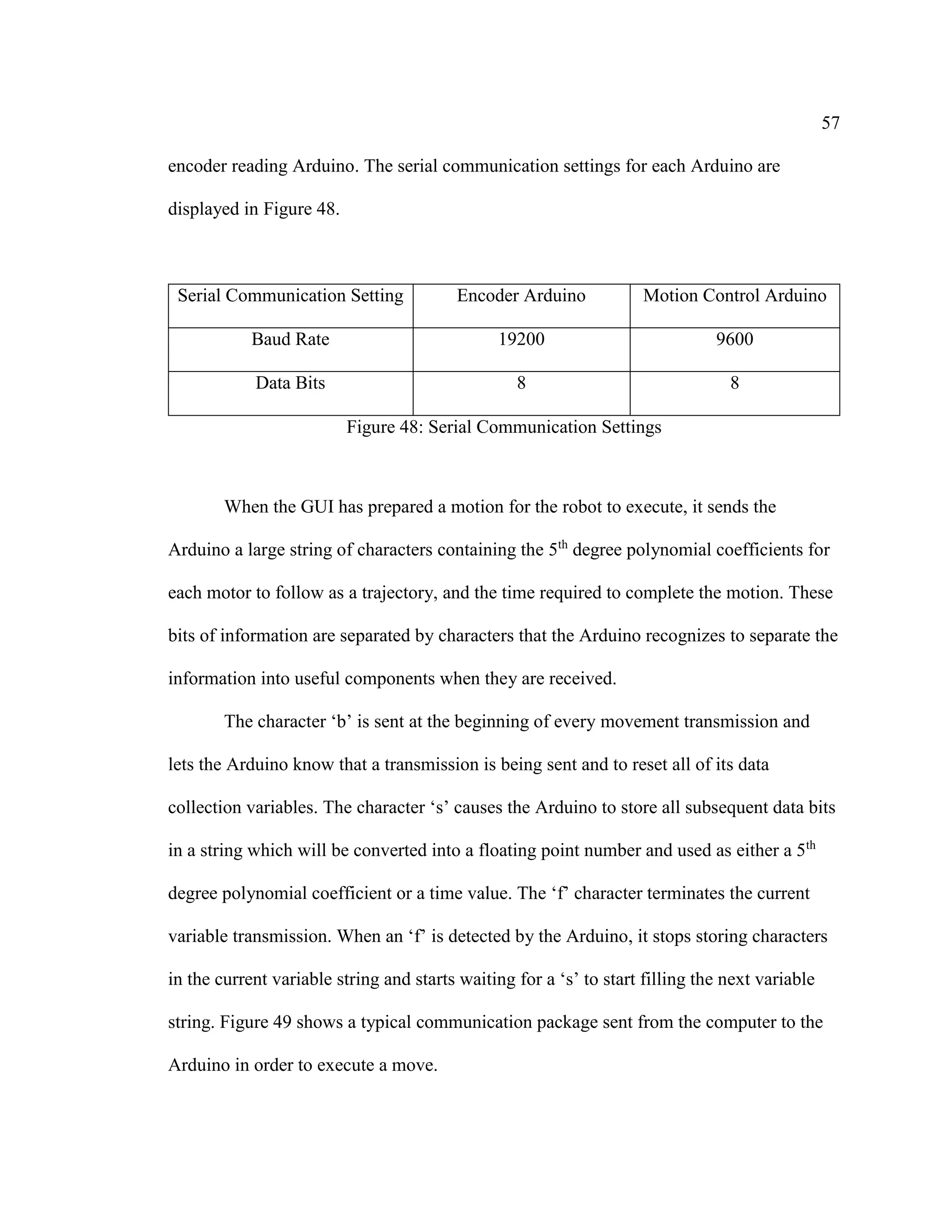
Figure 45: Robot GUI Startup Page.................................................................................. 54
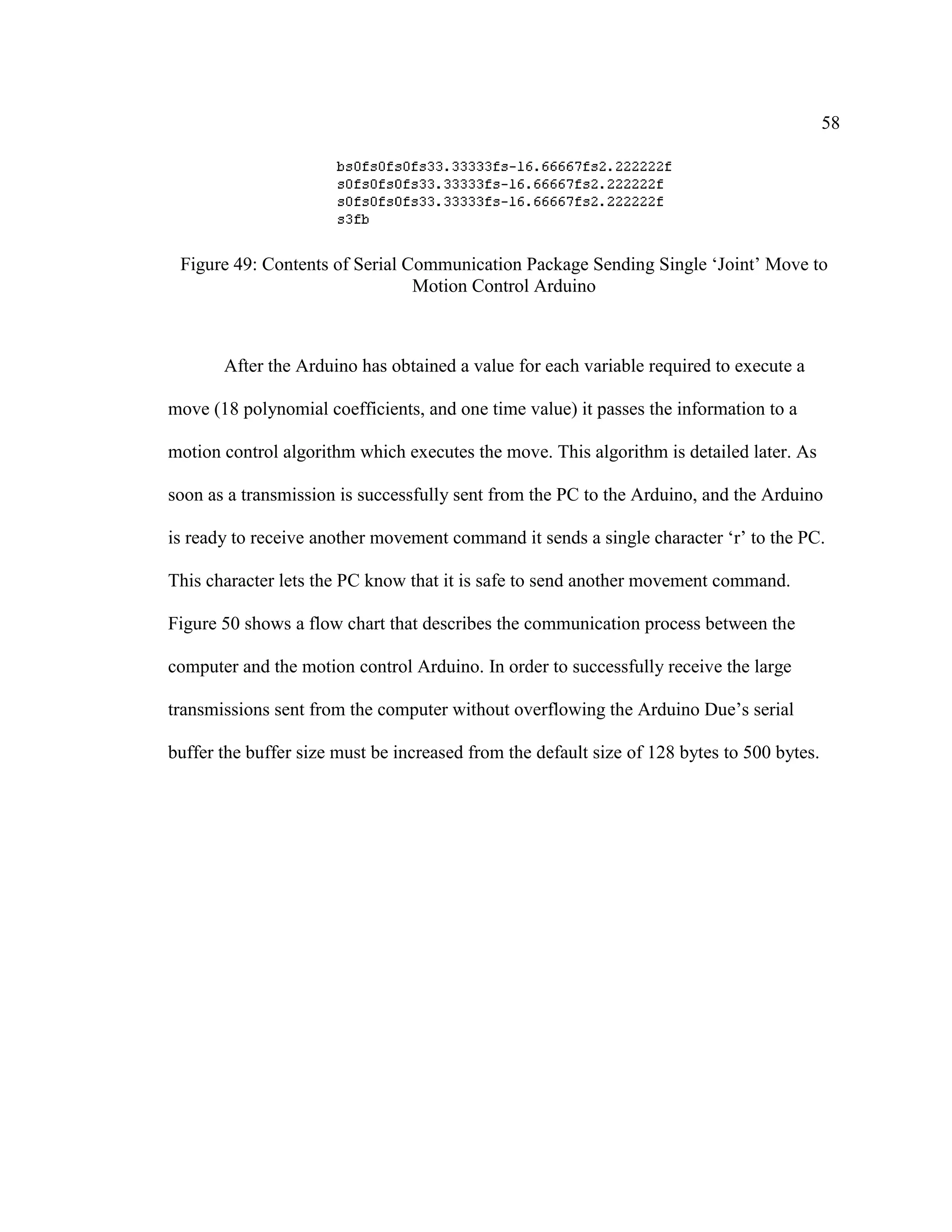
Figure 46: Linear/Circular GUI Interface......................................................................... 55

9. 9
Figure 47: A- Low Resolution Circle B- High Resolution Circle .................................... 56
Figure 48: Serial Communication Settings....................................................................... 57
Figure 49: Contents of Serial Communication Package Sending Single ‘Joint’ Move to
Motion Control Arduino ................................................................................................... 58
Figure 50: Flowchart of Serial Communication ............................................................... 59
Figure 51: Encoder Data Sent to Computer...................................................................... 60
Figure 52: Plots Generated by GUI After a Joint Move ................................................... 61
Figure 53: Positions of Two Sub-movements Flowing Into Each Other.......................... 63
Figure 54: Velocities of Two Sub-movements Flowing Into Each Other. ....................... 63
Figure 55: Accelerations of Two Sub-movements Flowing Into Each Other. ................. 63
Figure 56: Jerk of Two Sub-movements Flowing Into Each Other.................................. 64
Figure 57: A- Low Resolution Circle B- High Resolution Circle .................................... 66
Figure 58: A- Low Resolution Linear Move (.25 𝑀𝑜𝑣𝑒𝑠𝑐𝑚, or 3 Moves) B- High
Resolution Linear Move (5 𝑀𝑜𝑣𝑒𝑠𝑐𝑚)............................................................................ 66
Figure 59: Steps Taken to Process Linear Moves in GUI ................................................ 70
Figure 60: Circular Movement Process Flowchart ........................................................... 74
Figure 61: Motion Algorithm Flowchart .......................................................................... 77
Figure 62: Mechanical Proximity Switch ......................................................................... 78
Figure 63: Grid Generated of Work Space for Velocity Analysis at Each Node. ............ 80
Figure 64: Dial Indicator End Effectors............................................................................ 84
Figure 65: Angle Iron Used for XY Accuracy Testing..................................................... 84
Figure 66: Borosilicate Glass Sheet Used for Z Direction Resolution Testing................ 85
Figure 67: Pen End Effector ............................................................................................. 86
Figure 68: Maximum Velocity in X Direction at All Points in Horizontal Workspace ... 88
Figure 69: Maximum Velocity in Y Direction at All Points in Horizontal Workspace ... 88
Figure 70: Maximum End Effector Error in X Direction at Locations Inside Horizontal
Workspace (Errors in Units of ±𝑚𝑚).............................................................................. 90
Figure 71: Maximum End Effector Error in Y Direction at Locations Inside Horizontal
Workspace (Errors in Units of ±𝑚𝑚).............................................................................. 90
Figure 72: Accuracy Experimental Data........................................................................... 91

10. 10
Figure 73: Final Experimental Accuracies (With 99% Confidence)................................ 92
Figure 74: Dimensional Accuracy Verification................................................................ 93
Figure 75: Plotted Encoder Data....................................................................................... 94
Figure 76: Encoder Data for Motor #1 (662° − 1128°) vs. Theoretical Motion............. 96
Figure 77: Encoder Data for Motor #2 (662° − 825°) vs. Theoretical Motion............... 97
Figure 78: Encoder Data for Motor #3. (662° − 383°) vs. Theoretical Motion.............. 98
Figure 79: Joint One Circular Move Data (Encoder vs. Theoretical)............................. 100
Figure 80: Joint Two Circular Move Data (Encoder vs. Theoretical) ............................ 101
Figure 81: Joint Three Circular Move Data (Encoder vs. Theoretical) .......................... 102
Figure 82: Joint One Linear Move Data (Encoder vs. Theoretical) ............................... 103
Figure 83: Joint Two Linear Move Data (Encoder vs. Theoretical)............................... 104
Figure 84: Joint Three Linear Move Data (Encoder vs. Theoretical)............................. 105

11. 11
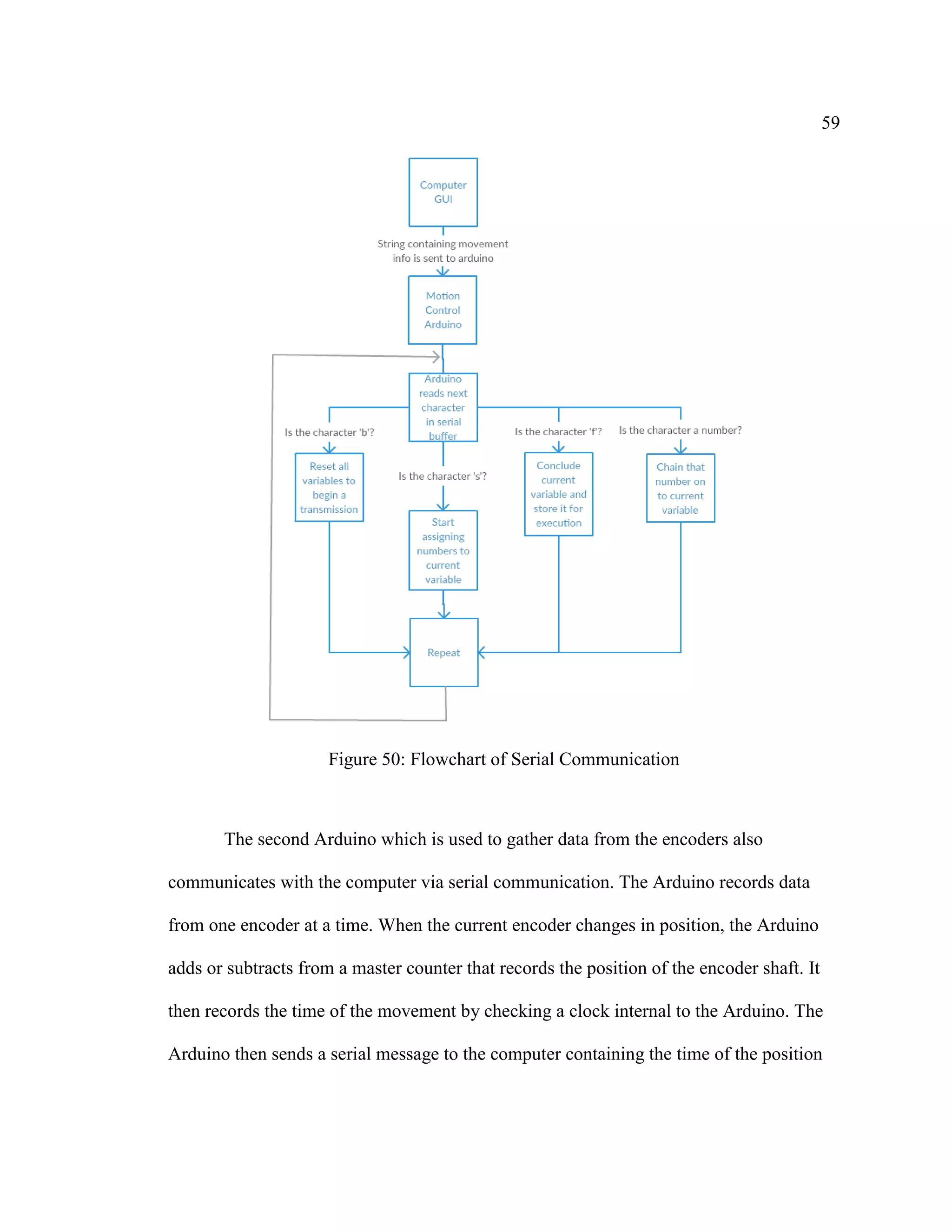
CHAPTER 1- INTRODUCTION AND LITERATURE REVIEW
Robots are important in many industries. They perform tasks that are too
repetitive or dangerous for humans to do, and virtually never make mistakes unless there
is a problem with their programming or hardware. They excel in pick and place
operations, welding, and CNC operations. With minimum wage increasing, they are even
used to serve us our food [1]. There are many different types of robots specialized for
different tasks.
Recently, robots have found a place in households in the form of 3D printing.
These 3D printers allow an individual with minimal skills to fabricate nearly any object
using a 3D printing process called FDM or fused deposition modeling. This involves
depositing layers of melted plastic onto a building surface layer by layer. By tracing out
the two dimensional cross sections of a three dimensional object and layering them on top
of each other, nearly any 3D object can be created. Recent developments in this field
such as the low cost microprocessor has caused a rapid expansion of the popularity and
affordability of this technology. 3D printing has become a very powerful tool both in
households and in industry and performs certain niche tasks more effectively than any
other fabrication technique. For example, 99% of custom hearing aids are created using
3D printing [2]. Other examples include fabricating bone implants, custom shoe insoles,
and tissue/organs [2].

12. 12
There are many different types of robots used for 3D printing. However the focus
of this thesis will not involve 3D printing, but the robot and control methods required for
3D printing or any other robot operation. These same control methods are used in CNC
mills, lathes, laser cutters, and other robots. The type of robot studied in this thesis will be
the linear input Delta Robot.
Literature Review
The Delta Robot was invented by Reymond Clavel in 1985 [4], [35]. Shown in
Figure 1, the original Delta Robot has three rotational input axes. The three arms attach to
three lower arms that consist of two parallel rods each forming a parallelogram. This
parallelogram restricted the motion of the end effector to three translational degrees of
freedom. The Delta Robot was invented primarily as a pick and place machine to move
chocolates from a conveyor belt into their packaging [4].
Figure 1: Clavel’s Delta Robot [8]

13. 13
Recently with the advent of 3D printing, the Delta Robot has been revisited. Its
design excels at this task because of its three translational degrees of freedom, and its
speed [5]. Hobbyists and engineers have developed many different designs for the Delta
Robot for 3D printing, most importantly using linear inputs driven by timing belts instead
of rotational inputs. Figure 2 demonstrates how the end effector of the linear input Delta
Robot moves with three translational degrees of freedom as a result of three linear inputs
driving carriages with two spherical or universal joints connecting two parallel rods to the
end effector. The linear input Delta Robot has become a common choice when
purchasing a 3D printer.
Figure 2: Linear Input Delta Robot [6]
Parallel vs Serial Robots
The Delta Robot belongs to a group called parallel robots [3]. Parallel robots use
multiple links attached to the end effector in order to move. In most cases, the motors
used to drive parallel robots are mounted to the stationary frame of the robot, and do not
move [3]. Parallel robots excel at pick and place operations where speed is important [3],

14. 14
[5], [7]. Just as the first Delta Robot was used to move chocolates from a conveyor belt to
their packaging [4], today’s parallel robots are used for similar tasks (pick and place
operations, and 3D printing).
Robots that are not parallel are known as serial robots. Serial robots have only one
link attached to the end effector, and often the motors are attached to moving parts of the
robot [3]. The traditional robotic arm is an example of a serial robot as shown in Figure 3.
Other serial robots include the traditional 3D printer which consists of a moving gantry
with two degrees of freedom and a build plate with one degree of freedom as shown in
Figure 4.
Figure 3: Fanuc Robotic Arm [9]

15. 15
Figure 4: Traditional Cartesian 3D Printer
Serial robots have both strengths and weaknesses. They have a large and simple
workspace [3], they also have high dexterity often in the form of six degrees of freedom
[3]. This makes serial robots effective in manufacturing environments where a task needs
carried out in a relatively large work cell (cage where the robot is enclosed for safety).
However serial robots also have numerous disadvantages. Each motor must overcome the
weight and inertia of the motors downstream of it, this results in slow speeds and a low
payload/weight ratio [3]. Along with this the error associated with each link is
compounding, resulting in large error in the location of the end effector [3].
Parallel robots also have many advantages and disadvantages. Their biggest
disadvantage is a small and complex work space [3] , [5]. Because of this, they can only
be used when the task can be completed in a very small area. However the advantages
make parallel robots the optimal choice in many situations. Because their motors are
mounted to the frame of the robot, the weight and inertia of the moving parts is low. This
results in higher top speeds and accelerations [3], [4], [5]. Along with their speed

16. 16
capabilities, parallel robots have a high payload/weight ratio, this is a result of multiple
links sharing the load of the end effector [3], [5]. Lastly, parallel robots are accurate [3].
This is because unlike serial robots, the error associated with the end effector does not
compound, but averages. Along with this, several links support the end effector resulting
in less strain. A more complete comparison of the advantages and disadvantages of serial
and parallel robots is provided in Figure 5.
Figure 5: Serial and Parallel Robot Comparison [3]

17. 17
Current Methods of Control
In order for a robot to complete a task, there must be a method of control used to
plan the motion of each actuator. This involves using the inverse pose kinematics to find
the initial and final angle of each motor shaft when given the (x, y, z) coordinates of the
end effector’s starting and ending point [10]. Each motor shaft must move from the initial
angle to the final angle in order for the end effector to reach the desired location [10].
The purpose of the control method is to dictate how the motor shafts will move
from their initial to their final angle in a smooth and timely manner. This is also referred
to the trajectory that each motor shaft follows. In motion control, trajectories are often in
the form of ‘trapezoidal velocity profiles’ [7], [11], [17]. This control method results in a
period of constant acceleration, followed by a period of constant speed, followed by a
period of constant deceleration as shown in Figure 6.
Figure 6: Trapezoidal Velocity Profile [12]

18. 18
Another common trajectory generation method is through the use of 3rd
order
polynomials [10][13]. If four initial conditions are known (initial/final position/velocity),
the coefficients of a third degree polynomial can be derived which will act as the
trajectory for the motor shaft to follow from the initial to the final angle as shown in
Figure 7.
Figure 7: 3rd
Order Polynomial Trajectory Profile [10]
Both trapezoidal velocity and 3rd
order polynomial trajectory control are used
because of their simplicity and seemingly smooth motion. However both share one
disadvantage: the occurrence of infinite jerk spikes [10]. Jerk is defined as the rate of
change of acceleration. An infinite jerk spike is a result of a discontinuity of acceleration.

19. 19
This is problematic because similar to velocity discontinuities being a physical
impossibility, acceleration discontinuities are a physical impossibility which are avoided
if possible in many areas such as motion control and cam design [10][14].
Control methods involving infinite jerk spikes attempt to force a motor to
accomplish something that is physically impossible. In most cases this is acceptable. The
resulting motion appears to be smooth, and because of their simplicity it has been
adopted as the norm for 3D printers and many robots to follow trajectories that involve
infinite jerk spikes such as trapezoidal velocity profiles [21].
Ensuring that no infinite jerk spikes occur can be essential in many applications.
Elevators are one instance where infinite jerk spikes are important to prevent [15].
Quality elevators have the capability to accelerate smoothly enough that passengers do
not feel themselves moving [15]. Without this smooth motion, motion sickness could
occur.
There are many negative effects of motion control involving infinite jerk spikes.
Motors undergo unnecessary wear by being controlled to do something they cannot do
[10]. This also creates unwanted vibrations in the frame of the robot. Currently, the speed
of FDM 3D printing (fused deposition modeling) is limited by the extruder and the heat
transfer rates [16]. This is the most common type of 3D printing involving layering
melted plastic. However as technology improves, robot speed may become the limiting
factor. At high speeds, the disadvantages of infinite jerk spikes may become more
pronounced and a more advanced method of control may be needed to prevent poor print

20. 20
quality caused by excessive vibrations, along with poor stepper motor performance which
are especially sensitive to resonance, and require smooth speed ramp up [17], [18].
One solution to the problem of infinite jerk spikes is the 5th
order polynomial
trajectory [19], [37], [38], [39]. Trajectory control via 5th
order polynomials prevents
infinite jerk spikes by ensuring that the acceleration undergoes no discontinuities. A 5th
order polynomial can be calculated using six initial conditions (initial and final position,
velocity, and acceleration).
Current 3D Printer and Home CNC/Robot Control
The advent of the cheap microprocessor has spurred a sharp increase in the
amount of robots and mechatronics projects available to engineers and hobbyists. These
microprocessors such as the Arduino, and the Raspberry Pi (a fully functional computer)
can be obtained for under $20 and are very small. Low cost 3D printers, CNCs, and other
robots have adopted these microcontrollers as a norm for low cost control [20].
Nearly all hobbyist microcontrollers used to control robots contain firmware
containing some variation of a g-code interpreter called ‘Grbl’ [21]. Grbl is a highly
optimized program whose primary purpose is to convert g-code into movement signals
that a robot’s motors can execute [21]. Grbl can fit onto an Arduino Uno, and can be used
to control a 3D printer, CNC, or other robot when configured correctly. Grbl is an
efficient tool for control, but suffers from infinite jerk spikes as a result of trapezoidal
velocity profile trajectory generation.

21. 21
Industrial motor controllers are high cost and use powerful hardware to control
robots. Some use methods to prevent infinite jerk spikes such as s-curves to gradually
change acceleration [22]. These controllers are too expensive to justify using in
household robots and CNCs. This generates a need for an affordable method of
controlling motors with the low cost microcontrollers that are currently in use.
Current Delta Robots
There are several different Delta Robot models currently in circulation. Figure 8
shows information about many popular models. The robots shown in Figure 8 are
depicted in Figure 9 and Figure 10. It can be seen that most Delta Robots have a
mechanical accuracy of approximately .1mm. This sets a standard that will be the goal of
the robot designed in this thesis. Achieving a resolution on the order of magnitude of
.1mm will be considered a success due to the prototype nature of the designed robot.
Figure 8: Delta Robot Information
Build Area Footprint Height (in) Accuracy Speed (mm/s)
Mini Kossel 6" Ø, 8.2" height 12"x12" 25.5" .1mm 300
Orion Delta 6" Ø, 9" height 14"x14" 24" .05mm 300
Deltaprintr 7" Ø, 10" height 11"x11" 24" .1mm 200
Deltamaker 9.5" Ø, 10.2" height 16"x16" 27" .1mm 300
Fanuc M-1iA/.5 11" Ø, 4" height 20"x17" 24.75" .02mm 3000
Thesis Robot 12"Ø, 15" height 27"x27" 36" Studied Studied

22. 22
Figure 9: A- Deltamaker 3D Printer[40]
B- ORION 3D Printer[23]
C- Kossel Mini 3D Printer [24]
Figure 10: A- Deltaprintr 3D Printer [25]
B- Fanuc M-1iA Delta Robot [26]

23. 23
Most Delta Robots have top speeds of 200-300mm/s as shown in Figure 8.
Although the robots are capable of high speeds, often they are operated at much slower
speeds. The 3D printer used to construct many parts of the Delta Robot designed in this
thesis gave the best results at speeds of 20mm/s and lower. Due to the complicated nature
of 5th
order polynomial control, reaching speeds of 200-300mm/s is unlikely and
unnecessary for the purposes of this thesis. As technology increases, low cost
microcontrollers will increase in computational power. This will result in lower
calculation times and higher top speeds for the robot being controlled via the presented
method. Because of this, high speeds will be attainable using the same methods presented
in this thesis when more powerful hardware becomes available. Because of this, low
speeds may be considered acceptable for the purposes of this thesis.
Thesis Purpose
The purpose of this thesis is the design of a new Delta Robot which makes
improvements over existing designs, most notably a change in the orientation of the
spherical ball joints which increases the useable work area by 336%. This new Delta
Robot is controlled via 5th
order polynomials to address the issue of infinite jerk spikes
seen in common robot control. A new control method is developed to allow low cost
microcontrollers to achieve this 5th
order polynomial control. Simulation and testing of
the robot’s speed and accuracy is done. Figure 11 shows the final design of the robot.

24. 24
Figure 11: Final Robot Design

25. 25
Objectives and Problem Statement
Based on the information presented above, it is clear that as 3D printing speeds
increase, there is a need for a method of control for robots using low cost
microprocessors that does not produce infinite jerk spikes. It is also clear that the design
of linear Delta Robots has not yet been perfected, and has room for improvement. The
goal of this thesis is to design a linear Delta Robot with improvements over previous
designs, and exploring design choices not yet visited. These design choices will be
analyzed and the constructed robot will be tested to quantify its speed, and accuracy. The
robot will be controlled to produce motion following 5th
order polynomial trajectories to
prevent infinite jerk spikes.
Objective 1- Design and Construction of Linear Input Delta Robot
The most effective design choices of popular models will be incorporated into the
design of this new model of linear Delta Robot along with new design choices not yet
explored. The robot will be designed with low cost in mind, as one purpose of the thesis
is to use low cost hardware to achieve high quality performance.
Objective 2- Achieve Control via 5th
Order Polynomial Trajectories
The method of 5th
order polynomial trajectories given by Craig [19] will be used
to plan the motion of the robot to prevent infinite jerk spikes. The control method will
allow the robot to execute the types of motion described in Figure 12. These types of

26. 26
motion are required to execute g-code generated for the purpose of 3D printing or CNC
operation [21].
Motion Type User Input Description
Joint Initial, final joint angles
Each joint follows 5th
order
trajectory from point A to point B.
Nonlinear end effector motion.
Cartesian Initial, final (x, y, z)
Each joint follows 5th
order
trajectory from point A to point B.
Nonlinear end effector motion.
Linear Initial, final (x, y, z)
End effector follows straight line
from point A to point B.
Circular
Initial, final, and pivot point (x, y, z)
End effector follows specified arc
from point A to point B about the
pivot point.
Figure 12: Motions Executable by Robot.
Objective 3- Analyze Robot Experimentally and Theoretically
The theoretical accuracy of the robot is computed by compounding the error
associated with each component of the robot using error propagation formulations. This
error will be tested experimentally to quantify the actual accuracy of the robot. The
maximum speed of the robot will be quantified based on the control algorithms. Lastly,
the actual motion of the robot will be compared to the theoretical motion via optical
encoders coupled to the motor shafts. This data will be used to verify that the actual
motion of the robot matches the theoretical motion.

27. 27
CHAPTER 2- METHODS
In this chapter the methods used to complete the thesis objectives are described.
Design choices for the linear Delta Robot are explained, and electronic control schemes
are detailed. The equations used will be presented and experimental data collection
methods explained.
Robot Design
The process of designing the linear Delta Robot is started by studying the design
of existing models. Many design choices existing in common 3D printers are accepted to
be the most effective design choice, and are expected (if not required) to be present in
any household linear Delta Robot. These include: the use of timing belts to actuate robot
carriages vertically along a linear rod/rail as shown in Figure 13, the presence of two
parallel links joining each carriage to the robot’s end effector as shown in Figure 15, the
use of NEMA 17 stepper motors as the primary actuators as shown in Figure 14, and a
frame consisting of extruded t-slot aluminum.

28. 28
Figure 13: Timing Belt Driving Linear Motion Along Hardened Rods
Figure 14: NEMA 17 Stepper Motor
Figure 15: Two Parallel Links Connecting Each Carriage to End Effector

29. 29
Unique Design Choices
Several design choices were made in the construction of this robot which are
uncommon or not seen at all in commercial linear Delta Robots. These design choices
were chosen with the goal of improving different aspects of the design. Some design
choices may unexpectedly result in poor results. This thesis will serve as a trial to show
the positive and negative effects of the design choices used.
The first design choice that deviates from commercial Delta Robots is a
hexagonal frame shown in Figure 17. This design choice is similar to that used in the
deltamaker robot shown in Figure 16. Most linear Delta Robots use a triangular frame to
increase stiffness and simplicity. A hexagonal frame allows for a large build plate to be
attached without overhang on the sides of the robot. The hexagonal frame works in
conjunction with the next unique design choice: double reinforced linear axes.
Figure 16: Deltamaker 3D Printer (Hexagonal Frame) [40]

30. 30
Figure 17: Top View of Robot, Showing the Hexagonal Shape of the Frame.
In most commercial linear Delta Robots the three carriages which slide along the
linear axes ride directly on the robot’s three support legs. The only support structure
existing between the top and bottom of the robot is either six hardened rods, or three
aluminum extrusions. The carriages slide along either of these two structures using linear
bearings or rollers as shown in Figure 18. The robot designed in this thesis is very large
in comparison to other linear Delta Robots as shown earlier in Figure 8 and therefore uses
both linear rods and aluminum extrusions to add stiffness to the frame. The rods are
coupled to the aluminum extrusions using rod end supports such as the ones shown in
Figure 18. This double reinforcement of the linear axes helps prevent a large problem
with large low budget linear Delta Robots, weakness in the frame.

31. 31
Figure 18: A- Deltaprintr Linear Inputs Riding Directly on Vertical Supports [25]
B- Rod End Supports used to Secure Hardened Rods
The third unique design choice used in this robot is three Plexiglas walls (shown
in Figure 19) coupled to the three unsupported hexagonal sides of the robot. These walls
serve four purposes: to act as a partial safety barrier between the user and the robot in the
case of dangerous operations such as laser cutting and milling, to serve as a partial
enclosure for 3D printing where air flow from the environment can cause adverse effects
on the quality of a 3D printed part, to act as an electrically insulated surface on which to
mount the electronics (shown in Figure 19), and most importantly to add stiffness to the
frame. The three Plexiglas walls can be easily removed for full access to the central area

32. 32
of the robot. This form of reinforcement is advantageous because it is rigid and does not
restrict the visibility of the internal parts of the robot.
Figure 19: A- Plexiglas Reinforcements Used to Stiffen Frame
B- Electronic Hardware Mounted to Plexiglas Sheet
Because the hexagonal shape of the frame is inherently weaker than a triangular
frame, a 1/5” sheet of oak plywood is coupled to the top of the robot to force the frame to
retain its hexagonal shape and not warp when forces are applied. This is in combination
with a ½” oak plywood bed coupled to the bottom of the frame which also acts to stiffen
the robot. The bed of the robot is supported by three 3D printed structures and is

33. 33
suspended on three springs. Wing nuts are used to adjust the tilt of the bed to ensure the
build surface is perfectly flat (shown in Figure 20). The two plywood sheets can be seen
in Figure 20, and Figure 21.
Figure 20: A- Wing Nut Used to Adjust Build Surface Atop 3D Printed Mount
B- ¾” Oak Plywood Sheet and 12”x12” Borosilicate Glass Supported by Rubber
Bumpers
Figure 21: Plywood Support Used to Force Top of Robot to Retain Hexagonal Shape

34. 34
The unique hexagonal frame of the robot requires irregular fittings to fasten the
frame together as shown in Figure 22. Just as in many other linear Delta Robots, fittings
have been designed and 3D printed to serve this purpose. The design uses 3D printed
fittings for nearly all of the structures of the robot. These 3D printed parts are easily
manufactured if access to a 3D printer is available. They are also lighter, and cheaper
than metal fittings. To show this, Figure 25 shows the weight, and cost of the 90°
supports used in this design, along with the metal fittings that are an alternative approach.
The 3D printed parts are assumed to have 100% infill (no internal voids). The cost
comparison is done using the price of non-brand name 1.75mm PLA filament available
online (
$18
𝑘𝑔
).
Figure 22: Obtuse 3D Printed Support Used to Connect Hexagonal Frame

35. 35
Fitting Type
Figure 23: 3D Printed
Fitting
Figure 24: Steel Fitting
Volume 4139.63𝑚𝑚3
1820.68𝑚𝑚3
Mass 5.3814g 14.651g
Cost $0.10 $5.82
Figure 25: Mass and Cost Comparison of 3D Printed (PLA) and Machined Metal 90°
Fittings (McMaster Carr).
In order to collect data from the motor shafts and compare it to the theoretical
values, rotary quadrature encoders have been coupled directly to the shafts of each input
motor. The encoders have a base resolution of 600 PPR with a possible resolution of
2400 PPR using quadrature techniques. In order to couple the motor to the encoder, a 3D
printed fixture is used to hold both the encoder and the motor as shown in Figure 26. The
fixture is then fastened to the frame of the robot as shown in Figure 26.

36. 36
Figure 26: A- Model of Motor/Encoder Coupling
B- 3D Printed Fixture Coupling Encoder to Motor Shaft
The most important design change featured by the new robot is a redesign of the
end effector and linear carriages. Most notably, a re-orientation of the spherical joints
used to attach the carriages to the end effector. Rendered models of both the end effector
and carriages are shown in Figure 27. Figure 28 shows one robot carriage after assembly
with the ball joints installed.
Figure 27:
A- Rendered Model of 3D Printed Robot Carriage
B- Rendered Model of 3D Printed End Effector

37. 37
Figure 28: 3D Printed Robot Carriage with Ball Joints
Commercial 3D printers use three types of joints to connect the end effector to the
carriages: 3D printed universal joints (Figure 29-A), magnetic ball joints (Figure 29-B),
and rod end ball joints (Figure 30). Rod end ball joints were chosen to use in this design
because of their low cost, and tight fit (no detectable error).
Figure 29: A- 3D Printed Universal Joints [28]
B- Magnetic Ball Joints [29]

38. 38
Figure 30: Traxxas Rod End Ball Joints
The main disadvantage of low cost rod end ball joints is their limited range of
motion. The ball can rotate freely about its central axis (parallel to the hole drilled in it)
but is limited to ± 20° about the other two primary axes (measured with a protractor).
Many other linear Delta Robots use similar ball joints. Commercial linear Delta Robots
that use rod end ball joints place them in a configuration that restricts the range of motion
due to the ± 20° limits of the joint. This restrictive orientation is shown in Figure 31. In
this orientation, the primary axis of the ball joint (which has no angle restrictions) is not
taken advantage of. By rotating the ball joints 90 degrees, and tilting them we can place
the joint in an orientation that takes advantage of the unbounded motion of the joint as
shown in Figure 31-B. Figure 32 and Figure 33 show the joint limits of the ball joints in
the new orientation.

39. 39
Figure 31: A- Restrictive Orientation of Rod End Ball Joints [30]
B- New Orientation of Rod End Ball Joints
Figure 32: A- Joint Limitation of End Effector (Side View)
B- Joint Limitation of Carriage (Top View)

40. 40
Figure 33: A- Joint Limit of End Effector (Top View)
B- Joint Limit of Carriage (Side View)
By using this new ball joint orientation the usable work area of the robot is
increased by 336%, where the usable work area is defined as the area of the largest circle
reachable by the robot. This is a result of a 109% increase in the diameter of the usable
work area. There are other areas that are technically reachable outside of this circle, but
for simplicity are not considered. This is because ‘slicing’ software (used to generate
executable g-codes for 3D printers) uses either a circular or rectangular work area for
user friendliness. The increased work area is demonstrated in Figure 34.This reorientation
of the ball joint has no effect on the usable work area of the robot in the vertical direction.

41. 41
Figure 34: Usable Work Space for New (Left) and Old (Right) Ball Joint Orientation.
Where the orange areas are unreachable, the yellow areas are reachable but excluded for
simplicity, and the green area is the usable space. The edges of the triangles represent the
pivot points of the ball joints where they connect to the carriages. These two models are
on a 1:1 scale.
The optimal angle of tilt used for the newly oriented ball joint (shown in Figure
35) is determined using an iterative process in Matlab in which the usable work space and
unusable work space are repeatedly plotted while changing the angle of tilt until the circle
inside the usable work space is at a maximum as shown in Figure 36. This tilt is applied
to the end effector as well as the carriage as shown in Figure 37 .

42. 42
Figure 35: Optimal Angle of Tilt for New Ball Joint Orientation (60°)
Figure 36: Matlab Plot Used to Iteratively Determine the Optimal Ball Joint Tilt to
Maximize Usable Work Area.
The green area represents the usable work area, and the orange area represents the dead
zone unreachable due to the ±20° ball joint limitations. The large circles represent the
maximum reach of the current link on the robot, while the small circles represent the
minimum reach.

43. 43
Figure 37: End Effector Ball Joint Tilt (Side View)
The end effector and carriages themselves are 3D printed. The carriages use
LM8UU linear bearings to slide along 8mm diameter hardened rods. The bearings are
placed in a triangular pattern to eliminate binding due to torsion of the carriage. The
carriage is designed in two halves which are designed to reduce weight. The two halves
are fastened together with M4 bolts. The end effector is designed to allow for different
end effector attachments to be coupled to it. Two of these end effector attachments are
used in the experimental testing of this robot.
All design choices for this robot were modeled and simulated in SolidWorks. This
ensured that parts fit together and served as the source file for the 3D printed parts. The
robot was simulated virtually with SolidWorks to ensure ranges of motion were valid.
Figure 38 shows a rendered model of the frame of the robot designed in SolidWorks.

44. 44
Figure 38: Rendered Model of Robot Frame
The design of the robot was an iterative process. The robot was constructed using
an initial design, and parts were changed and added as needed. The end result is a robot
larger than most linear Delta Robots available commercially and is stiff enough for the
desired precision. Many of the 3D printed parts printed for this robot were fabricated with
the Ohio University Mechanical Engineering Department’s 3D printer (Makerbot Gen5).
The rest of the parts were printed using a MakerSelect i3 3D printer.

45. 45
Control of the Robot
Like most linear Delta Robots, NEMA 17 stepper motors are used as the primary
actuators. These motors are useful because of their open loop nature. Another quality that
makes stepper motors suitable for linear Delta Robots is their ability to produce large
torques at low speeds [31]. This is opposed to servo motors which can attain high speeds
but have low torques [31]. These servo motors require a gearing system to convert their
speed into torque, and require an optical encoder to provide positional feedback to form a
closed loop control system. This requires complicated control methods to accurately
control motion, along with powerful hardware to keep up with the calculations while also
reading each encoder. Because the Arduino and other low cost microcontrollers are an
important part of current household robots, powerful servo motors are uncommon due to
the Arduino’s inability to control them successfully due to lack of computational power.
Stepper motors however do not suffer from the disadvantages of servo motors.
They are simple to control. Because of their high torque at low speeds they can be used as
direct drive motors [31]. Direct drive motors do not require a gearing system in order to
actuate a system [31]. Stepper motors operate by modulating current through coils inside
the motor. The current flowing through these coils creates a magnetic field which turn a
permanent magnet inside the motor.
Each time the electric field is changed the motor takes one “step” forward. Most
NEMA 17 stepper motors have a resolution of 200 steps per revolution. Proper regulation
of the current through the motor coils can result in resolutions higher than 200 steps per
resolution, this process is called ‘microstepping’. Hobbyist stepper motor drivers such as

46. 46
the ‘Pololu a4988’ [32] shown in Figure 39 are an important tool for controlling stepper
motors. Pololu a4988 stepper motor drivers are used to control this robot’s motors.
Figure 39: Pololu A4988 Stepper Motor Driver [32]
Stepper motor drivers contain circuitry that regulates the current through stepper
motor coils automatically. Microstep resolution on the a4988 driver can be set as high as
3200 steps per revolution [32] (each step broken into 16 microsteps). All that is required
to drive a motor with a stepper motor driver like the a4988 is that it is supplied with a
digital signal for both step and direction. Setting the step pin to ‘high’ actuates the motor
forward or back one microstep depending on the state of the direction pin.
The a4988 stepper driver is a ‘chopping’ stepper motor driver. Chopping drivers
allow the user to set a current limit for the motor for safety, and allow the use of higher
voltages than the motor is rated for [32]. The current limiting protects both the driver and
the motor, and the use of higher voltages allows for higher step response speed, which
results in higher top speeds for motors [32]. Stepper motor drivers allow a robot to be
controlled with a low cost microcontroller such as an Arduino.
In this thesis, an Arduino Due is used for control of the robot in conjunction with
a PC. The Arduino Due has more computational power than other models because it is

47. 47
equipped with a 32 bit processor as opposed to an 8 bit processor [33]. This allows for
faster computations that allow a 5th
degree polynomial trajectory motion algorithm to be
possible. Along with a 32 bit processor, the clock speed of the Arduino Due is 84MHz,
up from 16MHz with other Arduinos [33]. This increase in speed and processing power
makes the Arduino Due the only Arduino model powerful enough to drive a robot at
useful speeds using 5th
order polynomial trajectories.
One other difference between the Due and other models is its use of 3.3V logic.
As a result of the Due operating with 3.3V logic, 5v signals such as the signals supplied
by the optical encoders must be reduced to safe levels using a voltage divider circuit. A
voltage divider circuit uses Kirchhoff’s voltage law in conjunction with two resistors to
reduce an input voltage to a lower level depending on the ratio between the two resistors
[34].
The control method used in this thesis will consist of several components. First, a
GUI (graphical user interface) WinForms application is created on a PC using C# and
Microsoft Visual Studio. The GUI allows the user controls the robot. The desired motion
is specified, and graphical data is generated describing the motion. The computer is
responsible for the kinematics of the robot and the trajectory generation. The computer
processes moves for the robot to execute and then sends information to the Arduino Due
through a serial communication link. The Arduino Due contains a motion control
algorithm that turns the computer’s data into robot motion.
A second Arduino Due is used to collect data from the three optical encoders
coupled to the motor shafts. The Arduino Due responsible for the encoders records data

48. 48
from one encoder at a time, and sends information back to the PC via serial
communication. To collect data from a robot movement the motion is repeated three
times, each time gathering data from a different encoder. Gathering data from one
encoder at a time is required because the Arduino Due is driven by a single core
processor, and information would be lost when gathering data from more than one
encoder at once. Figure 40 shows a flow chart of the method used to control the robot.
Figure 40: Overall Control Flowchart

49. 49
Linear Delta Robot Kinematics
One of the most important tools in controlling a robot is the Inverse and Forward
Pose Kinematic solutions. The Inverse Pose Kinematics is used to determine the angle of
each motor shaft for an end effector location in (x, y, z) coordinates. The Inverse Pose
Kinematics is especially important in the control of the robot because it is calculated for
every move made by the robot. The Inverse Pose Kinematics is required for control of
any robot. The Forward Pose Kinematics is used to determine the end effector location in
(x, y, z) coordinates if the angle of each motor shaft is known (J1, J2, J3).
There are many approaches possible to solve the forward and reverse pose
kinematics of a robot including numerical methods, symbolic methods, and graphical
methods [7]. R. Williams II. presents a solution to both the Forward and Inverse Pose
Kinematics for the linear Delta Robot [5]. Figure 41 and Figure 42 and equations (1)-(18)
detail the Forward and Inverse Pose Kinematics used in this thesis. Figure 43 shows a list
of the essential variables needed to perform kinematic analysis on this robot. The validity
of this approach is verified through the ‘circular check’, inserting the inverse pose
kinematics solutions into the forward pose kinematics and vice versa as shown in Figure
44. Because identical results are obtained, the solution is mathematically sound [5].

50. 50
Figure 41: 3D View of Linear Delta Robot Coefficients [5]
Figure 42: A- Top View of Robot Frame [5]
B- Top View of Robot End Effector [5]

51. 51
Inverse Pose Kinematics:
𝐿𝑖 = −𝑧 ± √𝑧2 − 𝐶𝑖 (1)
𝐶1 = 𝑥2
+ 𝑦2
+ 𝑧2
+ 𝑎2
+ 𝑏2
+ 2𝑎𝑥 + 2𝑏𝑦 − 𝑙2
(2)
𝐶2 = 𝑥2
+ 𝑦2
+ 𝑧2
+ 𝑎2
+ 𝑏2
− 2𝑎𝑥 + 2𝑏𝑦 − 𝑙2
(3)
𝐶3 = 𝑥2
+ 𝑦2
+ 𝑧2
+ 𝑐2
+ 2𝑐𝑦 − 𝑙2
(4)
𝑎 =
𝑆 𝐵
2
−
𝑠 𝑝
2
(5)
𝑏 = 𝑊𝑏 − 𝑤 𝑝 (6)
𝑐 = 𝑢 𝑝 − 𝑈 𝐵 (7)
𝑊𝐵 =
√3
6
𝑆 𝐵, 𝑈 𝐵 =
√3
3
𝑆 𝐵, 𝑤 𝑏 =
√3
6
𝑠 𝑏, 𝑢 𝑏 =
√3
3
𝑠 𝑏,
𝑤 𝑝 =
√3
6
𝑠 𝑃, 𝑢 𝑝 =
√3
3
𝑠 𝑃
(8)
Forward Pose Kinematics:
𝑧1,2 = −𝐵 ±
√𝐵2 − 4𝐴𝐶
2𝐴
(9)
𝑥1,2 = 𝑑𝑧1,2 + 𝑒 (10)
𝑦1,2 = 𝐷𝑧1,2 + 𝐸 (11)
𝐴 = 𝑑2
+ 𝐷2
+ 1 (12)
𝐵 = 2(𝑑𝑒 + 𝐷𝐸 + 𝑐𝐷 + 𝐿3) (13)
𝐶 = 𝑒2
+ 𝐸2
+ 𝑐2
+ 2𝑐𝐸 + 𝐿3
2
− 𝑙2
(14)
𝐷 =
𝐿3 − 𝐿1 − 𝑎𝑑
𝑏 − 𝑐
(15)
𝐸 =
𝑐2
− 𝑎2
− 𝑏2
− 2𝑎𝑒 + 𝐿3
2
− 𝐿1
2
2(𝑏 − 𝑐)
(16)
𝑑 =
𝐿2 − 𝐿1
2𝑎
(17)

52. 52
𝑒 =
𝐿2
2
− 𝐿1
2
4𝑎
(18)
Name Meaning
𝑆 𝐵 P joints (𝐵𝑖) equilateral triangle side (mm)
𝑠 𝑝 Platform equilateral triangle side (mm)
𝐿𝑖 Leg length (mm)
𝑙 Lower legs parallelogram length (mm)
Figure 43: Essential Variables used in linear Delta Robot IPK/FPK [5]
Figure 44: Circular Check [36]
5th
Order Polynomial Trajectory Generation
This section details the methods used to calculate a 5th
order polynomial
trajectory. Trajectory control via 5th
order polynomials prevents infinite jerk spikes by
ensuring that the acceleration undergoes no discontinuities. As seen in equations (19)-(31)
a 5th
order polynomial can be calculated using six initial conditions, shown in equations
(23)-(25). Once a polynomial trajectory has been found, the velocity, acceleration, and
jerk can be calculated using equations (20), (21), and (22).
𝜃(𝑡) = 𝑎5 𝑡5
+ 𝑎4 𝑡4
+ 𝑎3 𝑡3
+ 𝑎2 𝑡2
+ 𝑎1 𝑡 + 𝑎0 (19)
𝜃̇( 𝑡) = 5𝑎5 𝑡4
+ 4𝑎4 𝑡3
+ 3𝑎3 𝑡2
+ 2𝑎2 𝑡 + 𝑎1 (20)

53. 53
𝜃̈( 𝑡) = 20𝑎5 𝑡3
+ 12𝑎4 𝑡2
+ 6𝑎3 𝑡 + 2𝑎2 (21)
𝜃⃛(𝑡) = 60𝑎5 𝑡2
+ 24𝑎4 𝑡 + 6𝑎3 (22)
𝜃(0) = 𝜃𝑠, 𝜃(𝑡𝑓) = 𝜃𝑓 (23)
𝜃̇(0) = 𝜃̇ 𝑠, 𝜃̇(𝑡𝑓) = 𝜃̇ 𝑓 (24)
𝜃̈(0) = 𝜃̈ 𝑠, 𝜃̈(𝑡𝑓) = 𝜃̈ 𝑓 (25)
𝑎0 = 𝜃𝑠 (26)
𝑎1 = 𝜃̇ 𝑠 (27)
𝑎2 =
𝜃̈ 𝑠
2
(28)
𝑎3 = −
20𝜃𝑠 − 20𝜃𝑓 + 12𝜃̇ 𝑠 𝑡𝑓 + 8𝜃̇ 𝑓 𝑡𝑓 + 3𝜃̈ 𝑠 𝑡𝑓
2
− 𝜃̈ 𝑓 𝑡𝑓
2
2𝑡3
(29)
𝑎4 =
30𝜃𝑠 − 30𝜃𝑓 + 16𝜃̇ 𝑠 𝑡𝑓 + 14𝜃̇ 𝑓 𝑡𝑓 + 3𝜃̈ 𝑠 𝑡𝑓
2
− 2𝜃̈ 𝑓 𝑡𝑓
2
2𝑡4
(30)
𝑎5 = −
12𝜃𝑠 − 12𝜃𝑓 + 6𝜃̇ 𝑠 𝑡𝑓 + 6𝜃̇ 𝑓 𝑡𝑓 + 𝜃̈ 𝑠 𝑡𝑓
2
− 𝜃̈ 𝑓 𝑡𝑓
2
2𝑡5
(31)
Where 𝜃𝑠and 𝜃𝑓 are initial and final input actuator positions such as motor shaft angle.
GUI Software
The control method used in this thesis consists of two main components: the PC
GUI software, and the Arduino motion control algorithm. This section will describe the
details of the GUI software. The software is developed in Microsoft Visual Studio as a
WinForms application. It is open source, and can be edited. The primary purpose of the
GUI is to do as many of the difficult calculations as possible, so that the calculations
done inside the Arduino are as simple as possible to increase robot speed. Figure 45
shows the startup page of the GUI.

54. 54
Figure 45: Robot GUI Startup Page
The GUI allows the user to execute several types of motion, the first of which is
the ‘Joint’ move. Joint moves allow the user to specify the initial and final angle of each
motor shaft, and each shaft follows a 5th
order polynomial trajectory from the initial to
the final angle. This type of motion does not result in linear motion from the end effector
and is primarily used in pick and place operations in industrial robots when speed is
desired, not accuracy or linear motion.
The second motion type possible through this GUI is the ‘Cartesian’ movement. It
is the same as the Joint movement however it requires the user to input an initial and final

55. 55
position in Cartesian (x, y, z) coordinates. Cartesian movements do not produce linear
motion.
The third and fourth types of motion are linear moves and circular moves. The
linear move requires the user to input an initial and final position in Cartesian (x, y, z)
coordinates, however it causes the end effector to move in a straight line from the initial
point to the final point. Circular moves require the user to input an initial position, a final
position, and a pivot point position in Cartesian coordinates (x, y, z). Figure 46 shows the
user interface for executing linear and circular movements. Circular movements can be
used to draw arcs and entire circles.
Figure 46: Linear/Circular GUI Interface

56. 56
Both linear and circular moves require the user to input a ‘resolution’ value. This
is because in order to execute linear and circular moves the robot must break the motion
into many small Cartesian movements flowing continuously into each other. The
resolution value is in units of
𝑚𝑜𝑣𝑒𝑠
𝑐𝑚
and dictates the quality of a linear or circular motion.
Higher resolutions result in smoother lines and circles. The default value for resolution is
set to 5 moves/cm. Figure 47-A shows the effects of using a resolution that is too low for
a circular move, and Figure 47-B shows a circular move with adequate resolution.
Figure 47: A- Low Resolution Circle
B- High Resolution Circle
Serial Communication
In this section, the details of how the GUI communicates with the Arduino are
explained. The GUI and the Arduino communicate through serial communication. When
the GUI is launched, the user is required to select two COM ports from a list of available
COM ports and connect to them, one for the motion control Arduino, and one for the

57. 57
encoder reading Arduino. The serial communication settings for each Arduino are
displayed in Figure 48.
Serial Communication Setting Encoder Arduino Motion Control Arduino
Baud Rate 19200 9600
Data Bits 8 8
Figure 48: Serial Communication Settings
When the GUI has prepared a motion for the robot to execute, it sends the
Arduino a large string of characters containing the 5th
degree polynomial coefficients for
each motor to follow as a trajectory, and the time required to complete the motion. These
bits of information are separated by characters that the Arduino recognizes to separate the
information into useful components when they are received.
The character ‘b’ is sent at the beginning of every movement transmission and
lets the Arduino know that a transmission is being sent and to reset all of its data
collection variables. The character ‘s’ causes the Arduino to store all subsequent data bits
in a string which will be converted into a floating point number and used as either a 5th
degree polynomial coefficient or a time value. The ‘f’ character terminates the current
variable transmission. When an ‘f’ is detected by the Arduino, it stops storing characters
in the current variable string and starts waiting for a ‘s’ to start filling the next variable
string. Figure 49 shows a typical communication package sent from the computer to the
Arduino in order to execute a move.

58. 58
Figure 49: Contents of Serial Communication Package Sending Single ‘Joint’ Move to
Motion Control Arduino
After the Arduino has obtained a value for each variable required to execute a
move (18 polynomial coefficients, and one time value) it passes the information to a
motion control algorithm which executes the move. This algorithm is detailed later. As
soon as a transmission is successfully sent from the PC to the Arduino, and the Arduino
is ready to receive another movement command it sends a single character ‘r’ to the PC.
This character lets the PC know that it is safe to send another movement command.
Figure 50 shows a flow chart that describes the communication process between the
computer and the motion control Arduino. In order to successfully receive the large
transmissions sent from the computer without overflowing the Arduino Due’s serial
buffer the buffer size must be increased from the default size of 128 bytes to 500 bytes.

59. 59
Figure 50: Flowchart of Serial Communication
The second Arduino which is used to gather data from the encoders also
communicates with the computer via serial communication. The Arduino records data
from one encoder at a time. When the current encoder changes in position, the Arduino
adds or subtracts from a master counter that records the position of the encoder shaft. It
then records the time of the movement by checking a clock internal to the Arduino. The
Arduino then sends a serial message to the computer containing the time of the position

60. 60
change of the encoder, along with the position encoder count, separated by a tab. Figure
51 shows a portion of communication that is sent from the Arduino to the PC.
Figure 51: Encoder Data Sent to Computer
This data will be copied and pasted into Microsoft Excel and plotted. The data
obtained from the encoders is compared with the theoretical motion of the robot by fitting
a 5th
order polynomial to the data and verifying that it is the same polynomial used by the
control algorithm to drive the motors.
Joint Moves
In this section, the details of how the GUI processes Joint moves is explained. The
user starts by inputting an initial and final angle for each motor along with a time
duration for its execution. When the user presses ‘start’ the GUI performs a series of
operations to prepare a movement, before sending it to the Arduino. First, the initial and

61. 61
final angles are used to generate a 5th
order polynomial using equations (26)-(31) and the
initial conditions shown in equations (32)-(34). The motion of the robot is then plotted as
shown in Figure 52. The GUI checks that the move does not exit the usable work space,
and then sends the Arduino the required information to execute the move.
𝜃(0) = 𝜃𝑠, 𝜃(𝑡𝑓) = 𝜃𝑓 (32)
𝜃̇(0) = 0, 𝜃̇(𝑡𝑓) = 0 (33)
𝜃̈(0) = 0, 𝜃̈(𝑡𝑓) = 0 (34)
Figure 52: Plots Generated by GUI After a Joint Move

62. 62
A joint move causes the robot’s joints to follow 5th
order polynomial trajectories
from their initial angle to their final angle. The resulting motion of the end effector does
not necessarily follow a straight line.
Cartesian Moves
In this section, the details of how the GUI processes Cartesian moves is
explained. Cartesian moves are handled much in the same way as joint moves. One
difference however is that before the trajectories are generated, the inverse pose
kinematics is done to convert the user inputs into lengths. Just like a joint move, a
Cartesian move causes the motors to follow 5th
order polynomial trajectories from their
initial angles to their final angles. The resulting motion of the end effector does not
necessarily follow a straight line. Generating a 5th
order trajectory for a joint or Cartesian
move is very simple, this is because many of the initial conditions are zero, only the
initial and final angle remain nonzero.
Velocity and Acceleration Equations
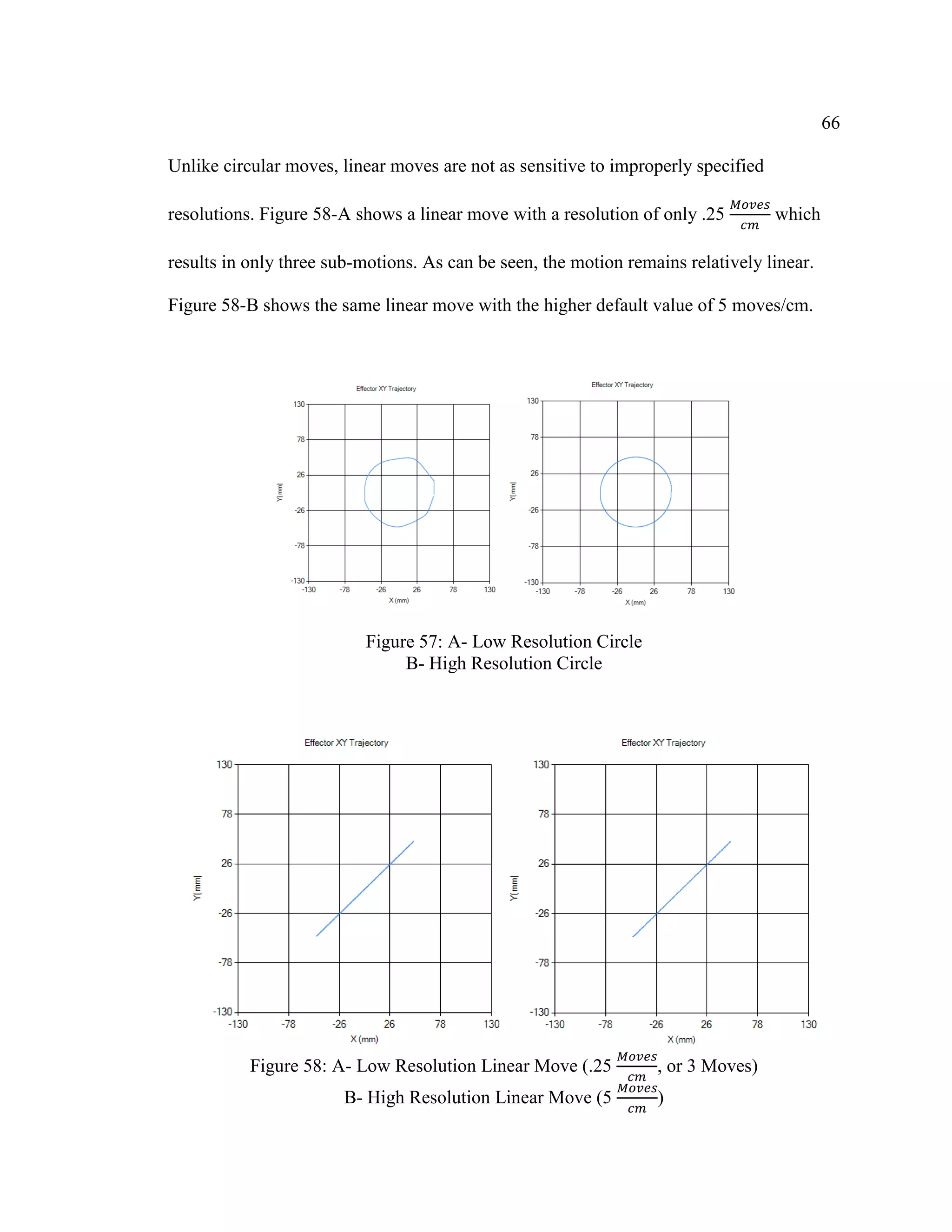
In order to execute a linear or circular movement, that movement must be broken
into many smaller sub-movements lying on the desired path [41]. These sub-movements
must flow together smoothly without stopping or jerking. In order to accomplish this, the
points where two sub-movements connect must share the same angular position, velocity,
and acceleration. Figure 53-Figure 56 demonstrate this and shows a movement which is
broken into two 5th order polynomial trajectories.

63. 63
Figure 53: Positions of Two Sub-movements Flowing Into Each Other
Figure 54: Velocities of Two Sub-movements Flowing Into Each Other.
Figure 55: Accelerations of Two Sub-movements Flowing Into Each Other.

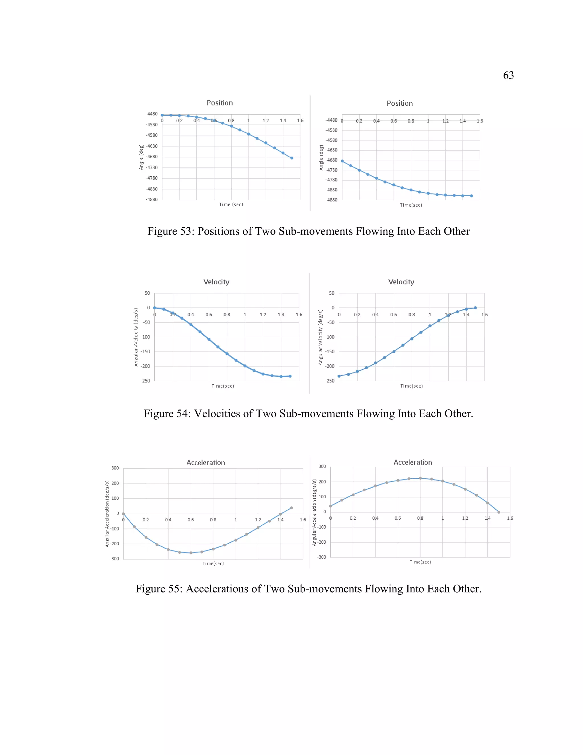
64. 64
Figure 56: Jerk of Two Sub-movements Flowing Into Each Other.
In order to know the angular position, velocity, and acceleration at the junctions
between sub-movements, an expression must be known relating them to end effector
position, velocity, and acceleration which is known. Derived by R. Williams II, the
relations between end effector velocity and linear input velocity are shown in equations
(35)-(37) [5]. Using these relations the angular shaft velocities can be calculated using
equation (38).
(𝑥 + 𝑎)𝑥̇ + (𝑦 + 𝑏)𝑦̇ + (𝑧 + 𝐿1)𝑧̇ = −(𝑧 + 𝐿1)𝐿̇1 (35)
(𝑥 − 𝑎)𝑥̇ + (𝑦 + 𝑏)𝑦̇ + (𝑧 + 𝐿2)𝑧̇ = −(𝑧 + 𝐿2)𝐿̇2 (36)
𝑥𝑥̇ + (𝑦 + 𝑐)𝑦̇ + (𝑧 + 𝐿3)𝑧̇ = −(𝑧 + 𝐿3)𝐿̇3 (37)
𝜃̇𝑖 =
𝐿̇ 𝑖
𝜋𝑟
(38)
Where L is the linear input position, r is the timing pulley radius, and a, b, and c
are constants given in equations (5)-(7).
To obtain the angular accelerations at the junctions between sub-movements there
must be an equation relating end effector acceleration to angular shaft accelerations.
Taking the time rate of change of equations (35)-(37) results in equations (39)-(41).

65. 65
Equation (42) can be used to convert the linear input accelerations into angular shaft
accelerations.
−
(𝑥 + 𝑎)𝑥̈ + (𝑦 + 𝑏)𝑦̈ + (𝑧 + 𝐿1)𝑧̈ + 𝑥̇2
+ 𝑦̇2
+ 𝑧̇2
+ 2𝐿̇1 𝑧̇ + 𝐿̇1
2
𝑧 + 𝐿1
= 𝐿̈1 (39)
−
(𝑥 − 𝑎)𝑥̈ + (𝑦 + 𝑏)𝑦̈ + (𝑧 + 𝐿2)𝑧̈ + 𝑥̇2
+ 𝑦̇2
+ 𝑧̇2
+ 2𝐿̇2 𝑧̇ + 𝐿̇2
2
𝑧 + 𝐿2
= 𝐿̈2 (40)
−
𝑥𝑥̈ + (𝑦 + 𝑐)𝑦̈ + (𝑧 + 𝐿3)𝑧̈ + 𝑥̇2
+ 𝑦̇2
+ 𝑧̇2
+ 2𝐿̇3 𝑧̇ + 𝐿̇3
2
𝑧 + 𝐿3
= 𝐿̈3 (41)
𝜃̈𝑖 =
𝐿̈ 𝑖
𝜋𝑟
(42)
The expressions presented in this section are required in order to execute linear
and circular moves with 5th
order polynomial trajectories in a smooth and continuous
manor. They serve as the initial and final conditions of junctions between 5th
order
polynomial trajectories for sub-motions involved in linear and circular movements.
Linear and Circular Moves
In this section, the details of how linear and circular moves are executed are
presented. Linear and circular moves are a product of separating a motion into several
sub-motions which lie on the desired path. These sub-motions flow smoothly into each
other to result in one continuous movement. As a result of the motion being separated
into several sub-motions, the user is required to designate a resolution which dictates how
many sub-motions occur. The default value for this resolution is 5 moves/cm.
Circular moves are especially sensitive to improperly specified resolutions.
Executing a circular move with a low resolution can result in irregular shapes such as in
Figure 57-A. Figure 57-B shows a circle with the default resolution of 5 moves/cm.

66. 66
Unlike circular moves, linear moves are not as sensitive to improperly specified
resolutions. Figure 58-A shows a linear move with a resolution of only .25
𝑀𝑜𝑣𝑒𝑠
𝑐𝑚
which
results in only three sub-motions. As can be seen, the motion remains relatively linear.
Figure 58-B shows the same linear move with the higher default value of 5 moves/cm.
Figure 57: A- Low Resolution Circle
B- High Resolution Circle
Figure 58: A- Low Resolution Linear Move (.25
𝑀𝑜𝑣𝑒𝑠
𝑐𝑚
, or 3 Moves)
B- High Resolution Linear Move (5
𝑀𝑜𝑣𝑒𝑠
𝑐𝑚
)

67. 67
As described previously, the GUI works in conjunction with the Arduino to
execute linear and circular moves. After the GUI has processed the set of sub-movements
required, it sends the initial move to the motion control Arduino. After the Arduino has
successfully received the move it begins to execute the move on the robot, along with
signaling to the computer that it is ready to receive the next move. The computer then
sends the next sub-movement and waits for permission to send the next move.
This pattern of the computer sending movements and the Arduino receiving,
executing, and requesting more movements is repeated until the overall linear or circular
move is complete. During this time, the GUI is unresponsive due to the single-thread
nature of the GUI and its continuous checking for communication from the Arduino.
Because the motion control Arduino collects movement information about the next move
while executing the current move instead of after it has finished, continuous motion from
one motion to the next is ensured.
For the purposes of this thesis, the absolute displacement of the end effector for
linear and circular moves has been controlled to follow a 5th
order polynomial trajectory.
This results in a two layer 5th
order control, both in the end effector motion and the sub-
movement motion. This method of end effector control is used arbitrarily to further
demonstrate the motion of 5th
order polynomials. End effector motion could easily be
adapted to follow other trajectories such as pseudo-trapezoidal velocity profiles, in which
instead of undergoing constant acceleration and deceleration stages, the acceleration is
continuously increased until the cruising speed is met, and continuously reduced at the
end of the motion.

68. 68
Linear Moves
In this section, the details of how the GUI processes linear moves is explained.
First, the user inputs (x, y, z) Cartesian coordinates for the starting and ending points of
the motion. Equations (43)-(45) is used to calculate the change in x, y, and z. Equation
(46) uses these results to calculate the distance of the linear move. Using equations (47)
and (48) the azimuth and phi angles are calculated. These two angles are needed to find
the x, y, and z components of any end effector motion. Using equations (49) - (51) x, y,
and z ‘factor’ are calculated. These factors are used to find the x, y, and z components of
any absolute end effector position, velocity, or acceleration.
∆𝑥 = 𝑥𝑓 − 𝑥𝑖 (43)
∆𝑦 = 𝑦𝑓 − 𝑦𝑖 (44)
∆𝑧 = 𝑧𝑓 − 𝑧𝑖 (45)
𝑑 = √∆𝑥2 + ∆𝑦2 + ∆𝑧 (46)
𝛾 = 𝐴𝑟𝑐𝑡𝑎𝑛 (
∆𝑦
∆𝑥
) (47)
𝜑 = 𝐴𝑟𝑐𝑐𝑜𝑠 (
∆𝑧
𝑑
) (48)
𝑥𝑓𝑎𝑐𝑡𝑜𝑟 = sin(𝜑) cos⁡( 𝛾) (49)
𝑦𝑓𝑎𝑐𝑡𝑜𝑟 = sin⁡( 𝜑)sin⁡( 𝛾) (50)
𝑧𝑓𝑎𝑐𝑡𝑜𝑟 = cos⁡( 𝜑) (51)
Where x, y, and z are the end effector coordinates, d is the distance of the move, 𝛾
is the azimuth angle, and 𝜑 is the phi angle (spherical coordinate measurements).
Using equation (52), the number of sub-movements to break the total move into is
found. The amount of time needed to execute each sub-movement is calculated using

69. 69
equation (53). In order to calculate the 5th
order polynomial path of the end effector,
equations (26)-(31) are used with the initial conditions given in equations (55)-(56) where
d is used in place of 𝜃.
𝑚𝑜𝑣𝑒𝑠 = (
𝑑
10
) 𝑟𝑒𝑠 (52)
𝑡𝑖 =
𝑡𝑓
𝑚𝑜𝑣𝑒𝑠
(53)
∆𝑧 = 𝑧𝑓 − 𝑧𝑖 (54)
𝑑(0) = 0, 𝑑(𝑡𝑓) = 𝑑 (55)
𝑑̇(0) = 0, 𝑑̇(𝑡𝑓) = 0 (56)
𝑑̈(0) = 0, 𝑑̈(𝑡𝑓) = 0 (57)
Where ‘moves’ is the number of sub-movements taken, d is the distance of the
move, ‘res’ is the resolution of the move in
𝑚𝑜𝑣𝑒𝑠
𝑐𝑚
, 𝑡𝑖 is the duration of each sub-
movement, and 𝑡𝑓 is the total duration of the move.
At this stage, a loop is repeated for each sub-movement. This loop calculates the
absolute displacement, velocity, and acceleration of the end effector at each sub-point
using equations (19) - (21). Each of these values is then broken into their x, y, and z
components using equations (49)-(51). Using the information now known, the inverse
pose kinematics along with the velocity and acceleration equations are used to convert
the x, y, and z components of position, velocity, and acceleration into linear input
positions, velocities, and accelerations. Using the IPK solution and equations (35) - (42)
the angular positions, velocities, and accelerations are found. At this time, all information
needed to generate a 5th
order polynomial for the current sub-movement is known. The

70. 70
trajectories for the current move are generated and stored in a buffer to be sent to the
Arduino.
This process is repeated for every sub-movement until all sub-movements are
calculated. Before sending the move to the Arduino, the GUI does a precautionary check
to ensure the movement is inside the usable work space of the robot. The buffer used to
store all sub-movement trajectories is then gradually emptied as movement information is
transferred to the Arduino as formerly described. Figure 59 shows a flow chart depicting
the process of executing a linear move.
Figure 59: Steps Taken to Process Linear Moves in GUI

71. 71
Circular Moves
In this section, the details of how the GUI processes circular moves is explained.
Circular moves are processed similarly to linear moves but with several changes. The
computer follows the same process of sending sub-moves to the motion control Arduino,
waiting for permission to send more, and repeating until the motion is complete. The
steps taken to generate the trajectories are slightly different.
First, the user inputs three (x, y, z) Cartesian coordinates: the starting point, the
ending point, and the pivot point. Along with setting the resolution of the move, the user
must designate for the motion to be clockwise or counterclockwise. Using equations (58)
and (59) the changes in x, y, and z between the pivot point and the starting point are
calculated.
∆𝑥𝑖 = 𝑥𝑖 − 𝑥 𝑣, ∆𝑦𝑖 = 𝑦𝑖 − 𝑦𝑣, ∆𝑧𝑖 = 𝑧𝑖 − 𝑧 𝑣 (58)
∆𝑥𝑓 = 𝑥𝑓 − 𝑥 𝑣, ∆𝑦𝑓 = 𝑦𝑓 − 𝑦𝑣, ∆𝑧𝑓 = 𝑧𝑓 − 𝑧 𝑣 (59)
Where 𝑥𝑖, 𝑦𝑖, 𝑎𝑛𝑑⁡𝑧𝑖 are the initial coordinates, 𝑥 𝑣, 𝑦𝑣, 𝑎𝑛𝑑⁡𝑧 𝑣⁡are the pivot point
coordinates, and 𝑥𝑓, 𝑦𝑓, 𝑎𝑛𝑑⁡𝑧𝑓 are the final coordinates.
The vectors between the pivot point and the starting and ending angles are defined
as vectors A and B. Using equation (60) and (61), the angles of vectors A and B are
found (measured from horizontal). The radius of the arc is then calculated using equation
(62) as the magnitude of vector A. The angle covered by the arc, the sweep, is calculated
using equation (63).
𝐴 𝜃 = 𝐴𝑡𝑎𝑛2 (
∆𝑦𝑖
∆𝑥𝑖
) (60)

72. 72
𝐵 𝜃 = 𝐴𝑡𝑎𝑛2 (
∆𝑦𝑓
∆𝑥𝑓
) (61)
𝑟 = √∆𝑥𝑖
2
+ ∆𝑦𝑖
2
(62)
𝑠𝑤𝑒𝑒𝑝 = 𝐴 𝜃 − 𝐵 𝜃 (63)
Where 𝐴 𝜃,⁡and⁡𝐵 𝜃 are the angles of vectors A, and B respectively, r is the radius
of the circle, and ‘sweep’ is the angular distance covered by the movement.
Next, the arc length of the circular move is found using equation (64). Similarly to
linear moves, the arc length is broken into sub-moves using equation (65). The time
duration of each sub-move is calculated using equation (66). An expression for the
displacement of the end effector is then calculated using a 5th
order polynomial trajectory
using equations (26) - (31) using the initial conditions shown in equations (67) - (69).
When calculating this 5th
order trajectory, s is used in place of 𝜃.
𝑠 = 𝑟 ∙ 𝑠𝑤𝑒𝑒𝑝 (64)
𝑚𝑜𝑣𝑒𝑠 = (
𝑠
10
) 𝑟𝑒𝑠 (65)
𝑡𝑖 =
𝑡𝑓
𝑚𝑜𝑣𝑒𝑠
(66)
𝑠(0) = 0, 𝑠(𝑡𝑓) = 𝑠 (67)
𝑠̇(0) = 0, 𝑠̇( 𝑡𝑓) = 0 (68)
𝑠̈(0) = 0, 𝑠̈( 𝑡𝑓) = 0 (69)
Where s is the arc length, r is the radius, sweep is the angle covered, ‘moves’ is
the number of sub-movements the circular move is broken into, res is the resolution of
the move in
𝑚𝑜𝑣𝑒𝑠
𝑐𝑚
, 𝑡𝑖 is the duration of each sub-movement, and 𝑡𝑓 is the total duration
of the move.

73. 73
Similarly to a linear move, a loop is then repeated for each sub-movement. This
loop calculates the absolute displacement, velocity, and acceleration of the end effector
along the arc at the current sub-movement using equations (19)-(21) (using s used instead
of 𝜃). The current angle (from horizontal) is then calculated using the current arc length
(displacement) and radius as shown in equation (70). The position, velocity, and
acceleration of the end effector are then multiplied by an x, y, and z factor determined by
equations (71)-(73). This determines the x, y, and z components of the position, velocity,
and acceleration tangent to the arc.
∅ = 𝐴 𝜃 +⁡
|𝑠|
𝑟
(70)
𝑥𝑓𝑎𝑐𝑡𝑜𝑟 = cos (∅ +
𝜋
2
) (71)
𝑦𝑓𝑎𝑐𝑡𝑜𝑟 = sin (∅ +
𝜋
2
) (72)
𝑧𝑓𝑎𝑐𝑡𝑜𝑟 = 0 (73)
Where ∅ is the current angle during the move, 𝐴 𝜃 is the angle of vector A from
the positive x axis, |s| is the arc length of the current point during the move, r is the
radius, and 𝑧𝑓𝑎𝑐𝑡𝑜𝑟 is zero because the control method considered only performs circular
moves in a constant z elevation.
Using the information known thus far, the inverse pose kinematics along with the
velocity and acceleration expressions shown in equations (35)-(42) are used to determine
the linear input position, velocity, and acceleration. Again using the transformation
shown in equations (38) and (42) the motor shaft positions, velocities, and accelerations
can be found. At this stage, all information required to generate a 5th
order polynomial for

74. 74
the current sub-movement is known, and the trajectory is generated and stored in a buffer
to be sent to the motion control Arduino.
Similarly to linear moves, before sending the final set of sub-movements to the
Arduino, the GUI performs a precautionary check to ensure the movement is inside the
usable work space of the robot. The buffer is then gradually emptied as movement
information is transferred to the Arduino as formerly described. Figure 60 shows a flow
chart depicting the process of executing a circular move.
Figure 60: Circular Movement Process Flowchart

75. 75
Arduino Motion Control
The Arduino Due responsible for controlling the motion of the robot performs
several tasks. First, it continuously listens for serial communication sent from the
computer as described previously. Second, it is responsible for sending digital signals to
stepper motor drivers which actuate the robot. This section will describe the motion
algorithm used to send digital signals to the stepper motor drivers, along with the zeroing
protocol used to zero the robot’s axes at the beginning of operation.
Motion Control Algorithm
The motion control algorithm is the process used by the Arduino to determine
when to send signals to the motor drivers to actuate the robot. There are two main
possible ways to execute this task. First, determine when each motor is required to move
and use a precise timers to actuate the motors. Because of the single threaded nature of
the Arduino, this method of control is nearly impossible. The Arduino does not possess
the processing and multithreading capability to process three different timer interrupts
along with the calculations involved with 5th
order polynomial trajectories. A timer
interrupt is a portion of code that is executed at a precise time while other code is
temporarily halted.
Instead of using the aforementioned process, the robot controlled in this thesis
uses a single timer interrupt. During this interrupt, all required calculations are performed
for each motor and digital signals are sent to the motor drivers if needed. This interrupt
occurs at a preprogrammed frequency. Using benchmarking processes, the total time

76. 76
needed to complete these calculations is determined to be 93 microseconds. To allow for
other operations to happen between interrupts, an extra 10 microseconds is added, and the
timer interrupt is told to occur every 103 microseconds (or .103 milliseconds). This
results in an algorithm frequency of 9,700Hz. This algorithm frequency limits the top
speed of the motors.
Inside of the Arduino, there are master position counters that track the current
position of the motor shafts. When the robot is zeroed, these counters are reset to zero.
Each time a timer interrupt occurs, the current time is plugged in to the 5th
degree
polynomial sent by the computer for each motor shaft. The result of these expressions are
the desired motor positions. If the current motor position of a motor does not match the
desired position by an amount greater than one microstep, the drivers are told to actuate
that motor one microstep towards the desired position. Once the move is complete (and
the current time matches the duration of the move) motion ceases. Figure 61 shows a
flow chart of this process.

77. 77
Figure 61: Motion Algorithm Flowchart
Zeroing Protocol
In order for the motion control algorithm to be sure of the position of the motor
shafts, a zeroing protocol must be undertaken to ‘zero’ the robot. This involves running
the motors slowly in reverse until contact is made with three mechanical proximity
switches shown in Figure 62. The zeroing protocol is executed when the motion control
Arduino is sent a ‘z’ character by the GUI. When a zeroing command is received, the
robot retracts each motor until contact with the proximity switches is made, the motors

78. 78
then move in the positive direction for 500 microsteps in order to break contact with the
proximity switches.
Figure 62: Mechanical Proximity Switch
Analysis
An analysis of the Delta Robot is done on several of its characteristics. The speed
of the robot is analyzed numerically. The motion of the robot is analyzed theoretically
and experimentally. The mechanical accuracy of the robot is analyzed both
experimentally and numerically. The details of these methods of analysis are explained in
this section.

79. 79
Velocity Analysis
An analysis of the maximum velocity of the motor shafts can be obtained directly
through knowledge of the operational frequency of the motion control algorithm. The
motor cannot move more frequently than the frequency of the algorithm. Using this
information and the distance covered each time the motor steps, the maximum motor
velocities are directly calculable. The maximum end effector speed however is not
uniform over the usable work area. To analyze this, a contour plot is generated in
Microsoft Excel to plot the maximum x and y velocities at different end effector
locations.
This process is completed by using the three velocity equations given by R.
Williams II (equations (35)-(37) shown below). A grid is generated showing the x and y
coordinates of the usable work space broken into 20mm increments as shown in Figure
63. As shown in the equations below, each linear input is able to cause a different
velocity on the end effector. To find the maximum velocity of the end effector in the x
direction, we substitute 𝑦̇=0 and 𝑧̇=0 into each of the three equations below. Knowing the
maximum input velocity 𝐿̇ 𝑖 (found from the maximum frequency of the motion
algorithm) the maximum end effector 𝑥̇ as a result of each linear input can be calculated
at each grid point. This is repeated for each linear input’s velocity equation to find the
maximum x velocity each linear input is able to impart on the end effector at maximum
linear speed.
(𝑥 + 𝑎)𝑥̇ + (𝑦 + 𝑏)𝑦̇ + (𝑧 + 𝐿1)𝑧̇ = −(𝑧 + 𝐿1)𝐿̇1 (35)
(𝑥 − 𝑎)𝑥̇ + (𝑦 + 𝑏)𝑦̇ + (𝑧 + 𝐿2)𝑧̇ = −(𝑧 + 𝐿2)𝐿̇2 (36)

80. 80
𝑥𝑥̇ + (𝑦 + 𝑐)𝑦̇ + (𝑧 + 𝐿3)𝑧̇ = −(𝑧 + 𝐿3)𝐿̇3 (37)
Figure 63: Grid Generated of Work Space for Velocity Analysis at Each Node.
This process of finding the maximum end effector speed imparted by each linear
input at each location is repeated for the y direction velocity. After six grids have been
generated (three for each linear input’s maximum x velocity contributions, and three for
each linear input’s maximum y velocity contributions) the minimum possible x direction
speed of the three cases is taken at each grid point and combined into one grid. This grid
contains the maximum x direction velocity at each point. This process is repeated for the
three y direction velocity grids and plotted as a contour chart for visualization.
-150 -130 -110 -90 -70 -50 -30 -10 10 30 50 70 90 110 130 150
150
130
110
90
70
50
30
10
-10
-30
-50
-70
-90
-110
-130
-150

81. 81
Motion Analysis
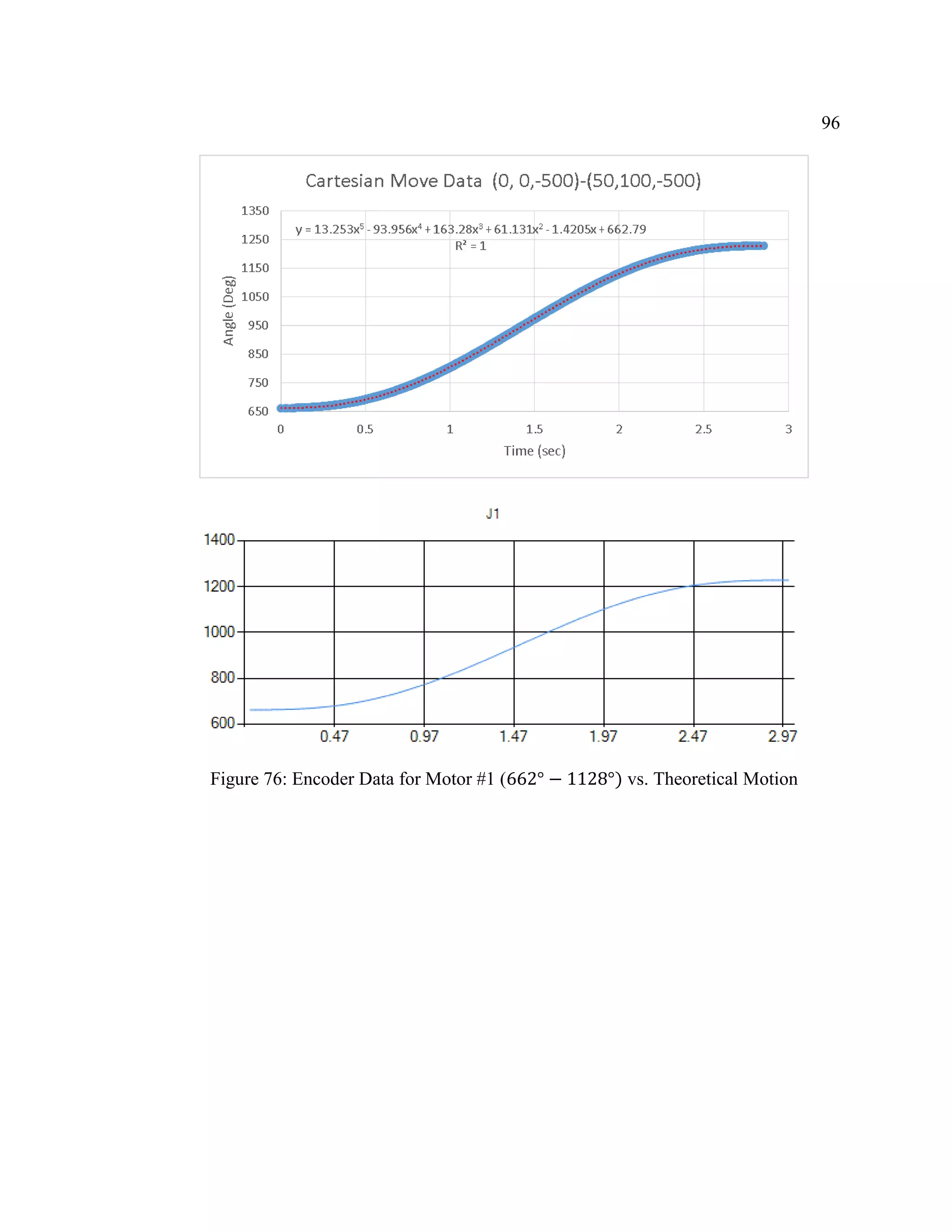
Analysis of the robot’s motion is performed using plots of the theoretical motion
generated by the GUI, and by data collected by optical encoders coupled to each motor
shaft. A designated Arduino will be used to collect data from one motor shaft at a time,
which is send to the computer via serial communication. The resulting data can be plotted
in Microsoft Excel, and compared with the theoretical motion.
5th
degree polynomial trend lines will be fit to the data obtained from the
encoders. If the motors are shown to follow 5th
order polynomial trajectories, the control
process is verified, and infinite jerk spikes are said to be prevented (because the third
derivative of a 5th
degree polynomial trajectory results in a finite jerk profile). This
process will be used to analyze Cartesian and joint moves.
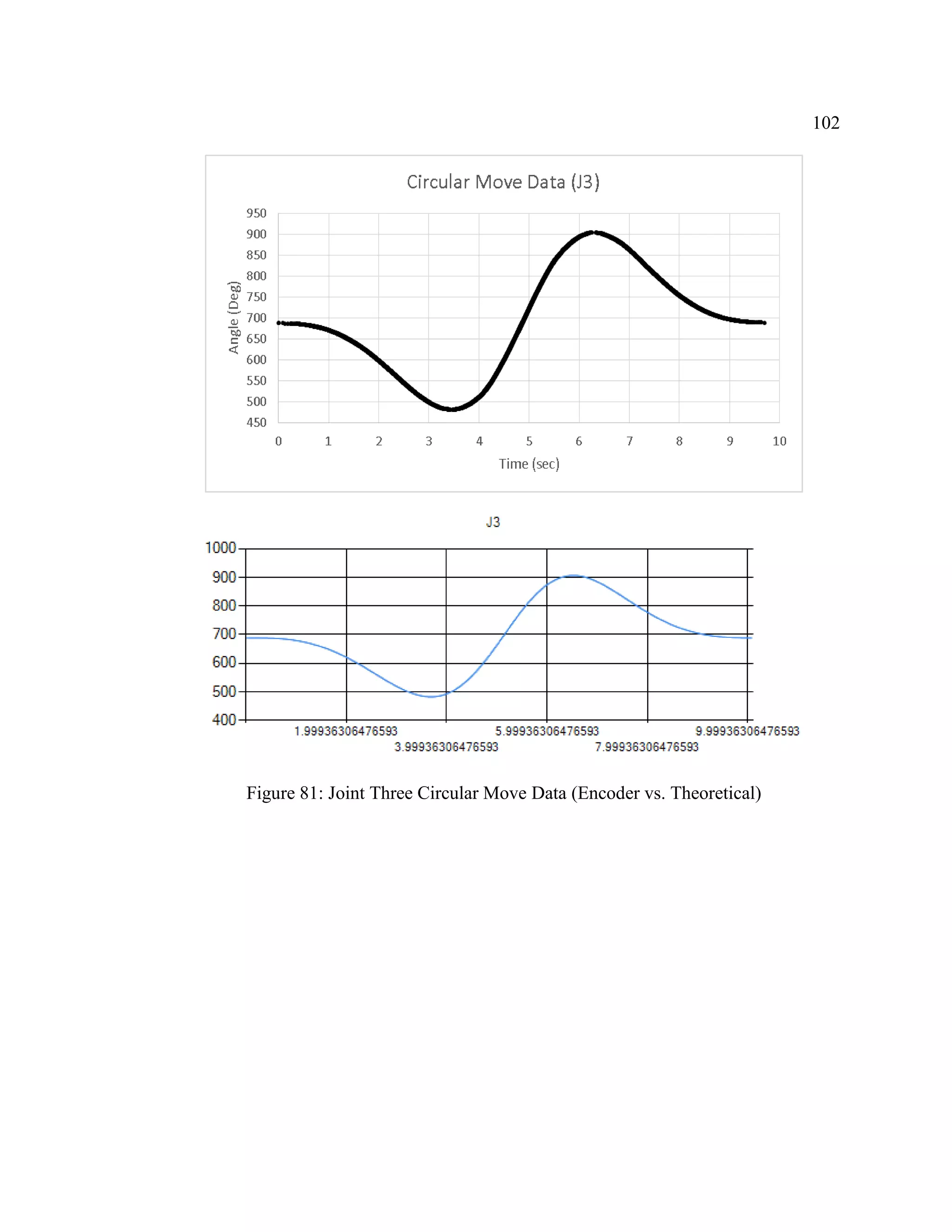
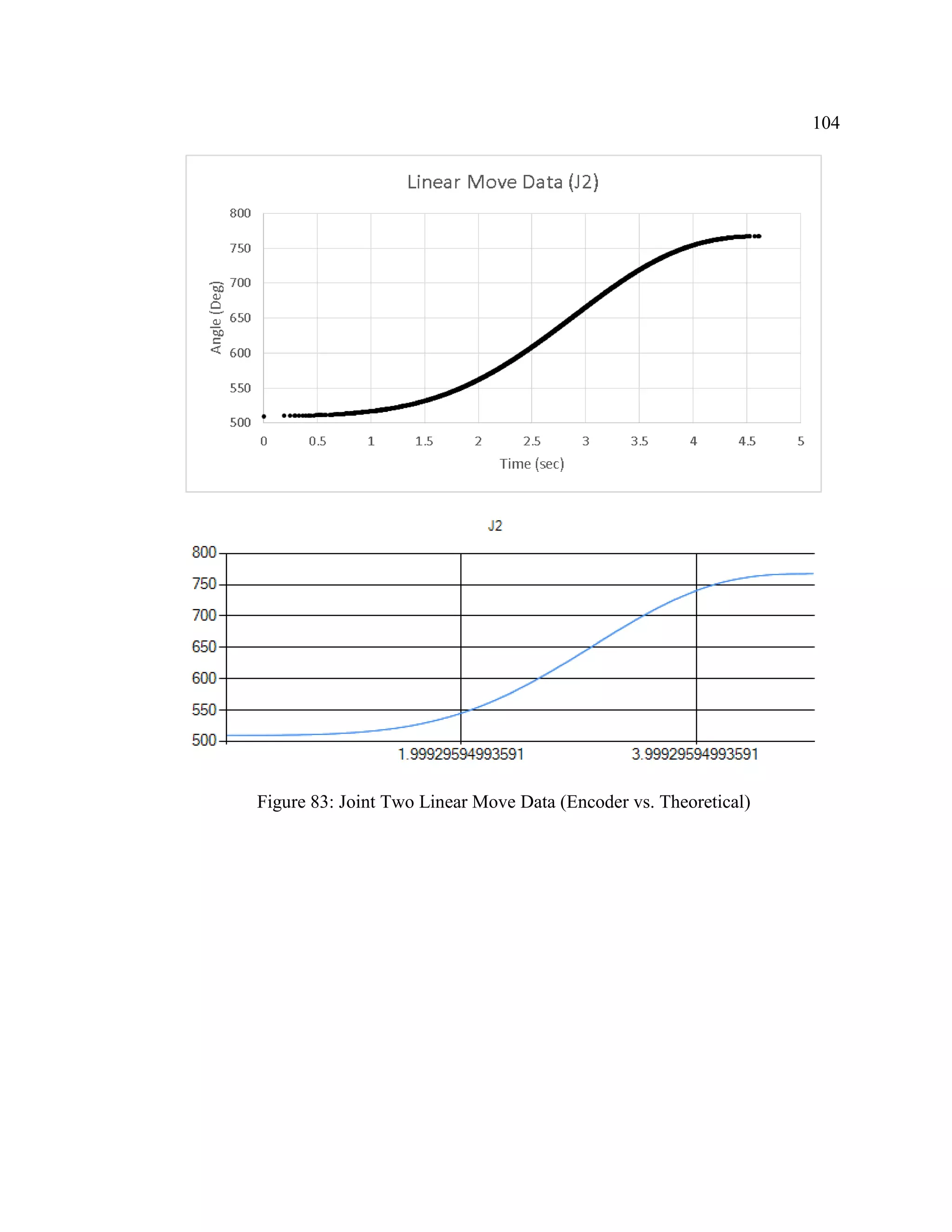
In order to analyze linear and circular moves, encoder data will be imported into
Microsoft excel, converted from units of encoder count to units of degrees, and compared
with the theoretical motion of the robot generated by the GUI. If the plots are the same,
the control method is successful.
Accuracy Analysis
The accuracy of the robot will be determined both symbolically and
experimentally. In order to obtain the symbolic solution for the accuracy of the robot in
the x, y, and z direction the error propagation formula (equations (75) and (76)) will be
applied to the forward pose kinematics solution [43]. Matlab is used to calculate the

82. 82
partial derivatives needed, and generate a contour plot of the error at each point on the
horizontal workspace.
Where 𝛿 denotes the uncertainty associated with a variable (±𝑥⁡𝑚𝑚).
The only source of error inside the Delta Robot assembly other than strain is the
resolution of the motors (3200 microsteps/revolution) which results in the input lengths
𝐿𝑖 being the only partial derivatives needed. Both the bearings and spherical joints have
virtually zero perceptible error. The only other source of error in the system is caused by
strain imparted on the system by internal forces. These errors are not within the scope of
this thesis and are not studied. Because the motion control algorithm rounds motion to the
nearest microstep when controlling the robot, the error associated with each linear input
is ±
1
2
of one microstep, which is found to be ±.00625mm using equation (77).
Where 𝛿 denotes the uncertainty associated with a variable (±𝑥⁡𝑚𝑚), R is the
resolution of the stepper motor (3200
𝑆𝑡𝑒𝑝𝑠
𝑅𝑒𝑣
), and D is the diameter of the timing pulley.
The frame dimension used in the forward kinematics are corrected during a
calibrating procedure done during robot setup. This involves moving the end effector to
several points on the build plate and measuring the z dimension with a ruler or dial
𝑋 = 𝑓(𝐿1, 𝐿2, 𝐿3), 𝑌 = 𝑓(𝐿1, 𝐿2, 𝐿3) (74)
𝛿𝑋 = √(
𝜕𝑋
𝜕𝐿1
𝛿𝐿1)
2
+ (
𝜕𝑋
𝜕𝐿2
𝛿𝐿2)
2
+ (
𝜕𝑋
𝜕𝐿3
𝛿𝐿3)
2
(75)
𝛿𝑌 = √(
𝜕𝑌
𝜕𝐿1
𝛿𝐿1)
2
+ (
𝜕𝑌
𝜕𝐿2
𝛿𝐿2)
2
+ (
𝜕𝑌
𝜕𝐿3
𝛿𝐿3)
2
(76)
𝛿𝐿𝑖 =
𝐷𝜋
2𝑅
(77)

83. 83
indicator. These values are entered into a website which uses a calibration algorithm
involving the least squares method to give corrections to key dimensions to result in
correct dimensional accuracy and account for any errors in the measurement of frame
dimensions [27]. Because this calibration method is used, the error associated with all
physical dimensions is assumed to be zero.
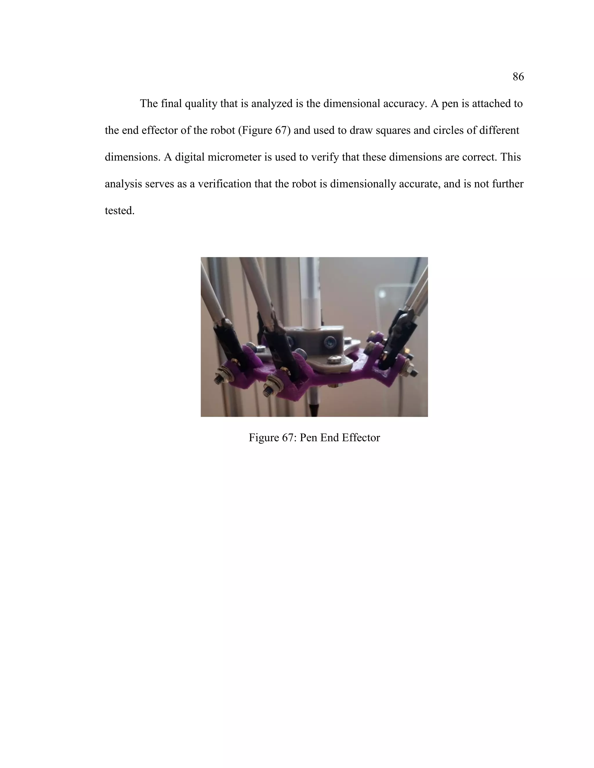
The accuracy of the robot will be obtained experimentally using a dial indicator
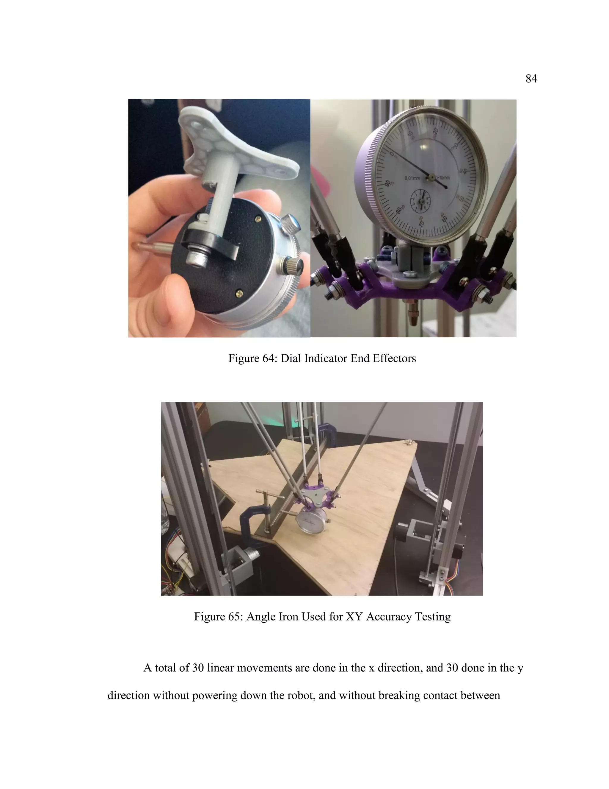
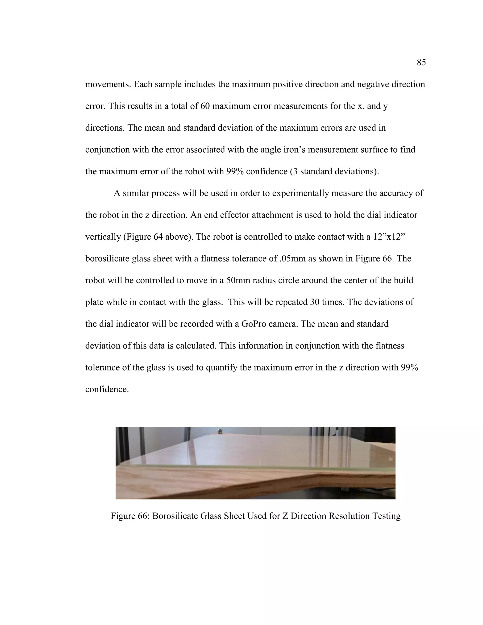
end effector attachment for both the horizontal and vertical directions as shown in Figure
64. The x and y direction resolutions will be obtained using a piece of steel angle iron
clamped to the build plate as shown in Figure 65. A flat surface has been machined into
the top surface of the angle iron with a tolerance of ±.05mm. The robot is controlled to
make contact with one end of the angle iron and move linearly along the surface to the
other end. A GoPro camera will be used to record the deviations in the x and y direction
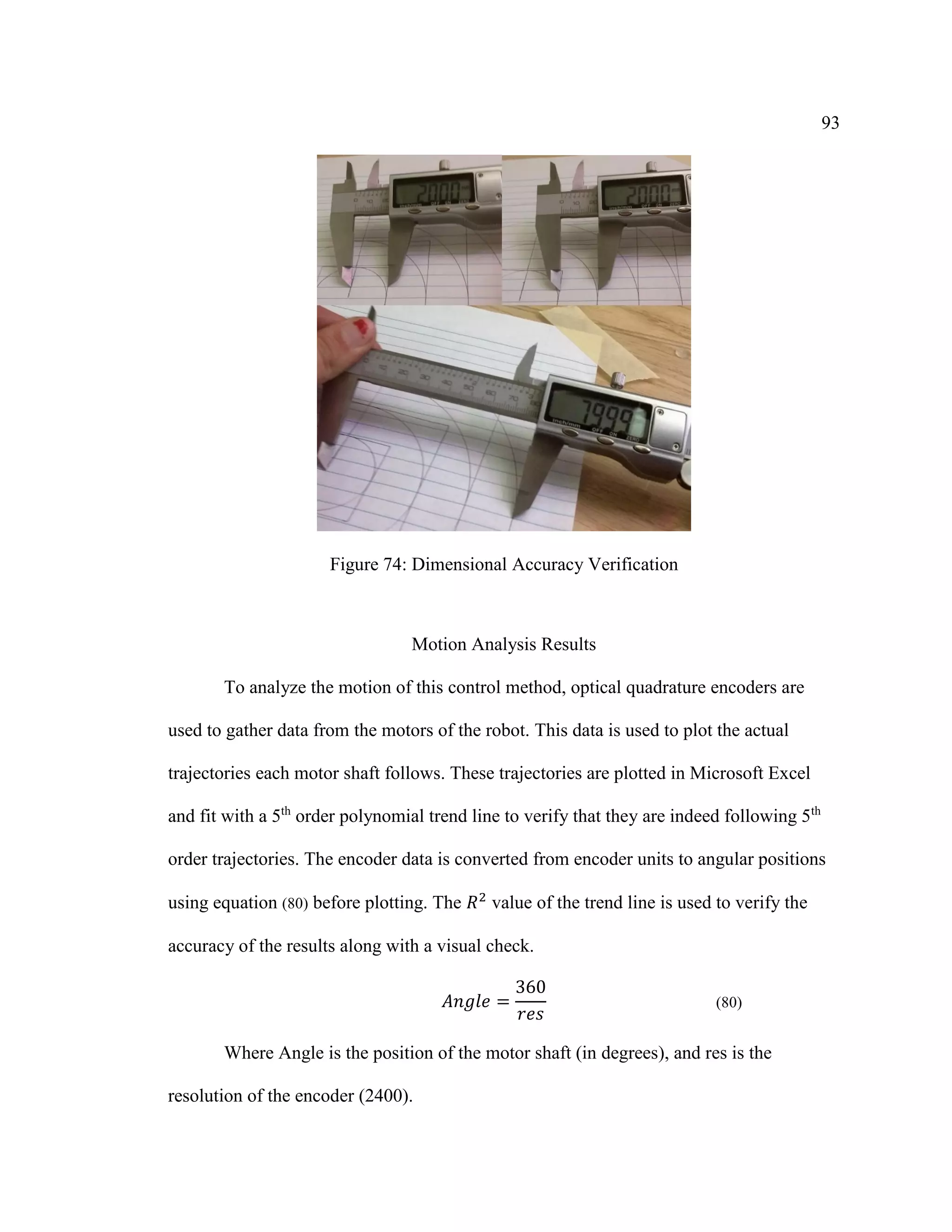
shown on the dial indicator.

84. 84
Figure 64: Dial Indicator End Effectors
Figure 65: Angle Iron Used for XY Accuracy Testing
A total of 30 linear movements are done in the x direction, and 30 done in the y
direction without powering down the robot, and without breaking contact between

85. 85
movements. Each sample includes the maximum positive direction and negative direction
error. This results in a total of 60 maximum error measurements for the x, and y
directions. The mean and standard deviation of the maximum errors are used in
conjunction with the error associated with the angle iron’s measurement surface to find
the maximum error of the robot with 99% confidence (3 standard deviations).
A similar process will be used in order to experimentally measure the accuracy of
the robot in the z direction. An end effector attachment is used to hold the dial indicator
vertically (Figure 64 above). The robot is controlled to make contact with a 12”x12”
borosilicate glass sheet with a flatness tolerance of .05mm as shown in Figure 66. The
robot will be controlled to move in a 50mm radius circle around the center of the build
plate while in contact with the glass. This will be repeated 30 times. The deviations of
the dial indicator will be recorded with a GoPro camera. The mean and standard
deviation of this data is calculated. This information in conjunction with the flatness
tolerance of the glass is used to quantify the maximum error in the z direction with 99%
confidence.
Figure 66: Borosilicate Glass Sheet Used for Z Direction Resolution Testing

86. 86
The final quality that is analyzed is the dimensional accuracy. A pen is attached to
the end effector of the robot (Figure 67) and used to draw squares and circles of different
dimensions. A digital micrometer is used to verify that these dimensions are correct. This
analysis serves as a verification that the robot is dimensionally accurate, and is not further
tested.
Figure 67: Pen End Effector

87. 87
CHAPTER 3- RESULTS
In this section, the results of this thesis are presented. Most of the results will be
related to the theoretical and experimental analysis of the robot’s physical characteristics.
The characteristics which are analyzed are: speed, accuracy, and motion.
Velocity Analysis Results
Quantification of the robot’s maximum speed is done by analysis of the motion
control algorithm. The timer interrupt which controls the motor has a period of 103
microseconds (a frequency of 9700Hz). Using equation (78) the maximum speed of the
motor shafts are found to be 3.031
𝑟𝑒𝑣
𝑠𝑒𝑐
. Using equation (79) the maximum linear input
velocity is calculated to be 121
𝑚𝑚
𝑠
.
𝑟𝑝𝑠 =
𝑓𝑟𝑒𝑞𝑢𝑒𝑛𝑐𝑦
𝑟𝑒𝑠𝑜𝑙𝑢𝑡𝑖𝑜𝑛
(78)
𝐿̇ 𝑖 = 𝑟𝑝𝑠 ∙ 2𝜋𝑟 (79)
Where rps is the maximum speed of the motors in
𝑟𝑒𝑣
𝑠𝑒𝑐
, frequency is the frequency
of the motion control algorithm (9700Hz), resolution is the number of microsteps to
complete one revolution on the stepper motor (3200), 𝐿̇ 𝑖 is the maximum linear speed of
each input, and r is the radius of the timing pullies.
Due to the complex nature of the robot’s kinematics its maximum velocity is not
constant throughout the horizontal work plane. Figure 68 and Figure 69 show the
maximum end effector velocities in the x and y directions at different locations on the
horizontal work space. Although different (x, y) coordinates have different maximum

88. 88
velocities, the maximum z direction velocity is constant at all points and is limited to the
linear speed of the inputs (121
𝑚𝑚
𝑠
).
Figure 68: Maximum Velocity in X Direction at All Points in Horizontal Workspace
Figure 69: Maximum Velocity in Y Direction at All Points in Horizontal Workspace

89. 89
To obtain the results shown in Figure 68 and Figure 69 the velocity equations
(35)-(37) are used to plot the maximum end effector speed in both the X, and Y directions
as a result of each linear input moving at maximum speed. This results in six sets of data
giving the maximum x, and y velocity at each point in three different cases: input one,
two, and three moving at maximum speed. This results in 3 sets of data for the maximum
speed in the x direction. The minimum of three cases is chosen at each point to generate
the plots shown of the maximum x and y speeds at each point in the horizontal work
space.
Accuracy Analysis Results
The resolution of the robot is tested in the x, y, and z direction both theoretically
and experimentally. Matlab was used to calculate and plot the maximum errors in the x
and y directions at all locations in the usable work space. The results of the theoretical
error analysis are shown in Figure 70 and Figure 71. These results show that there is a
theoretical error of ±.014mm near the center of the workspace, and errors as low as
±.008 at the outer reaches of the workspace.

90. 90
Figure 70: Maximum End Effector Error in X Direction at Locations Inside Horizontal
Workspace (Errors in Units of ±𝑚𝑚)
Figure 71: Maximum End Effector Error in Y Direction at Locations Inside Horizontal
Workspace (Errors in Units of ±𝑚𝑚)

91. 91
Figure 72 shows the data collected from the x, y, and z direction accuracy tests. A
dial indicator was used to experimentally test the resolution of the robot. To test the z
direction, the dial indicator was moved in a 50mm radius circular motion around the
center of the build plate on top of a 12”x12” borosilicate glass sheet with a surface
flatness of ±.05mm. To test the x and y direction, the dial indicator was moved along a
machined surface of a 12” piece of angle iron with a flatness of ±.05mm.
Figure 72: Accuracy Experimental Data
The tolerance of the borosilicate glass sheet used to test the Z direction accuracy
has a tolerance of ±.05𝑚𝑚. The metal surface used to measure the X and Y direction
Run Number Positive Error (mm) Negative Error (mm)
1 0.15 0.2
2 0.3 0.15
3 0.15 0.15
4 0.3 0.15
5 0.1 0.2
6 0.3 0.2
7 0.15 0.18
8 0.28 0.2
9 0.15 0.15
10 0.32 0.15
11 0.12 0.17
12 0.32 0.17
13 0.15 0.15
14 0.32 0.15
15 0.15 0.23
16 0.27 0.23
17 0.15 0.25
18 0.35 0.25
19 0.12 0.21
20 0.28 0.25
21 0.12 0.22
22 0.29 0.22
23 0.09 0.18
24 0.29 0.18
25 0.15 0.28
26 0.35 0.28
27 0.15 0.29
28 0.3 0.29
29 0.12 0.23
30 0.28 0.23
31 0.15 0.3
32 0.29 0.3
Mean 0.215625 99% Maximum Error
Stdev 0.070175561 0.426151683
X Direction Accuracy Data
Run Number Positive Error (mm) Negative Error (mm)
1 0.15 0
2 0.05 0.1
3 0.15 0.06
4 0.05 0.15
5 0.1 0.15
6 0.05 0.12
7 0.15 0.03
8 0.05 0.15
9 0.15 0.1
10 0.05 0.1
11 0.15 0.06
12 0.06 0.1
13 0.15 0.06
14 0.06 0.15
15 0.15 0.05
16 0.04 0.1
17 0.15 0.04
18 0.04 0.1
19 0.15 0.05
20 0.05 0.1
21 0.15 0.04
22 0.06 0.13
23 0.15 0.07
24 0.05 0.15
25 0.14 0.05
26 0.06 0.1
27 0.15 0.06
28 0.05 0.15
29 0.15 0.1
30 0.06 0.1
31 0.1 0.15
32 0.17 0.05
Mean 0.09625 99% Maximum Error
Stdev 0.045328661 0.232235983
Y Direction Accuracy Data
Run Number Positive Error (mm) Negative Error (mm)
1 0.08 0.07
2 0.08 0.08
3 0.1 0.07
4 0.1 0.09
5 0.07 0.1
6 0.08 0.09
7 0.09 0.09
8 0.08 0.08
9 0.08 0.07
10 0.07 0.07
11 0.1 0.07
12 0.07 0.07
13 0.08 0.07
14 0.09 0.07
15 0.07 0.07
16 0.08 0.07
17 0.09 0.07
18 0.06 0.07
19 0.07 0.07
20 0.09 0.07
21 0.08 0.06
22 0.08 0.07
23 0.1 0.07
24 0.08 0.07
25 0.07 0.07
26 0.09 0.06
27 0.08 0.07
28 0.08 0.06
29 0.09 0.07
30 0.08 0.06
Mean 0.077166667 99% Maximum Error
Stdev 0.01081537 0.109612776
Z Direction Accuracy Data

92. 92
accuracy has a tolerance of ±.05mm as well. Because of this, .05mm must be added to
the results shown in Figure 72 to be 99% sure of the accuracy values found. Figure 73
shows the final experimental accuracy values found.
X Direction Accuracy Y Direction Accuracy Z Direction Accuracy
±0.476 mm ±0.282 mm ±0.160 mm
Figure 73: Final Experimental Accuracies (With 99% Confidence)
The third and last step taken to analyze the accuracy of the robot is to test for
dimensional accuracy. This is done by attaching a pen to the end effector and drawing
several shapes. The shapes are measured using a digital caliper to verify the dimensional
accuracy of the robot. Figure 74 shows several squares drawn by the robot. The outside
edges of each square are drawn to be 20mm apart by the GUI. As seen in the figures, the
dimensional accuracy of the robot is verified to be accurate.

93. 93
Figure 74: Dimensional Accuracy Verification
Motion Analysis Results
To analyze the motion of this control method, optical quadrature encoders are
used to gather data from the motors of the robot. This data is used to plot the actual
trajectories each motor shaft follows. These trajectories are plotted in Microsoft Excel
and fit with a 5th
order polynomial trend line to verify that they are indeed following 5th
order trajectories. The encoder data is converted from encoder units to angular positions
using equation (80) before plotting. The 𝑅2
value of the trend line is used to verify the
accuracy of the results along with a visual check.
𝐴𝑛𝑔𝑙𝑒 =
360
𝑟𝑒𝑠
(80)
Where Angle is the position of the motor shaft (in degrees), and res is the
resolution of the encoder (2400).

94. 94
As a result of round off error inside the motion control algorithm when
calculating time, there are small inaccuracies in the time domain which cause the actual
movement duration to vary from the desired movement duration. This time difference is
seen in the plots of joint data.
Cartesian/Joint Motion Analysis Results
Joint and Cartesian movements are executed in much the same way. Both
movements cause each motor shaft to follow a single 5th
order polynomial from initial
angle to final angle. Because of this, Joint and Cartesian moves are investigated together.
To analyze these movements, a joint and Cartesian movement is performed. For the joint
move, the motors are controlled to move from 0° to 360° over a 3 second period. The
resulting motion is shown in Figure 75. Because each motor follows the same trajectory,
each plot is identical and thus only one is shown.
Figure 75: Plotted Encoder Data

95. 95
The data plotted in Figure 75 verifies that the trajectory followed by each motor
shaft follows a 5th
order polynomial. The red dotted line represents the trend line
generated by Microsoft Excel. The 𝑅2
value of .9999 along with a visual check shows
that the 5th
degree polynomial shown is taken. Taking the third derivative of the trend line
equation shown yields a function yielding finite jerk. Thus this motion is successfully
executed without infinite jerk spikes.
The procedure above is repeated for a Cartesian movement from (0, 0,-500) to
(50, 100, -500). The motion of each joint is shown separately because each follows a
different trajectory. Figure 76 - Figure 78 show the motion of each motor shaft, followed
by the theoretical motion generated by the GUI. These motions follow 5th
order
polynomials as shown by the trend line generated by Microsoft Excel and the 𝑅2
values
and a visual check.

96. 96
Figure 76: Encoder Data for Motor #1 (662° − 1128°) vs. Theoretical Motion

97. 97
Figure 77: Encoder Data for Motor #2 (662° − 825°) vs. Theoretical Motion

98. 98
Figure 78: Encoder Data for Motor #3. (662° − 383°) vs. Theoretical Motion
Circular/Linear Move Motion Analysis
Circular and Linear moves are broken up into many sub-movements each
following 5th
order polynomials in order to remain on the desired linear or circular path.
As a result of this, the overall motion of the motor shaft from initial to final angle does
not follow a single 5th
order polynomial and thus cannot be fitted with a 5th
order trend
line such as with Joint and Cartesian moves to prove that infinite jerk is prevented. As a

99. 99
result of this, other means must be used to ensure that linear and circular moves do not
contain infinite jerk spikes.
The methods used to generate the polynomials of each sub-movement prevents
infinite jerk spikes from occurring in theory. As a result of this, if the resultant motion of
linear/circular moves is smooth (as verified by the x, y, and z direction error tests, and
visual inspection) the method of control is proven to be successful, and thus no infinite
jerk spikes occur.
To further confirm that the actual motion of linear/circular moves follows the
theoretical motion, the encoder data is plotted next to the theoretical motion as shown in
Figure 79- Figure 84. The circular move executes a full circle starting and ending at (-50,
0, -500) with a pivot point of (0, 0, -500) over 10 seconds. The linear move travels from
(50, 0,-500) to (-50, -100, -500) over 5 seconds.

100. 100
Circular Move Plots
Figure 79: Joint One Circular Move Data (Encoder vs. Theoretical)

101. 101
Figure 80: Joint Two Circular Move Data (Encoder vs. Theoretical)

102. 102
Figure 81: Joint Three Circular Move Data (Encoder vs. Theoretical)

103. 103
Linear Move Plots
Figure 82: Joint One Linear Move Data (Encoder vs. Theoretical)

104. 104
Figure 83: Joint Two Linear Move Data (Encoder vs. Theoretical)

105. 105
Figure 84: Joint Three Linear Move Data (Encoder vs. Theoretical)

106. 106
CHAPTER 4- DISCUSSION
Several topics covered in this thesis may serve to improve the design of linear
Delta Robots, and the control of all low cost robots controlled with similar hardware.
Some choices made during this investigation resulted in less than optimal results. Both
the design of the robot, and the development of the GUI and motion control algorithm
were iterative processes with many roadblocks encountered before everything worked.
This chapter will discuss the choices made, what should be done differently in the future,
and possibilities for further research.
GUI Discussion
The GUI which controls the robot investigated was created using C# in Microsoft
Visual Studio. Using C# was a good decision as opposed to using a less sophisticated
language like ‘processing’ which was considered. It is a very powerful language with
many capabilities. The drawback of using the method of control shown in this thesis is
the requirement for a PC to do half of the work. To improve upon this drawback, a
Raspberry Pi could be used to run the GUI software. The cost of Arduino and Raspberry
Pi hardware are very low and their capabilities are steadily increasing.
One improvement that could be made to the GUI is the addition of multi-
threading support. Currently, only one processor thread is used to run this software. As a
result, the GUI freezes while executing a linear or circular move. An experienced
programmer may be able to find a way to fix this without multithread support.

107. 107
The second thing that could be improved about the GUI is the addition of a G-
code interpreter, and cornering algorithms. Currently, the control method used can
execute all g code commands needed in most applications (linear, and circular moves).
However, these linear and circular moves do not flow into each other, they must come to
a complete stop before executing the next movement. Grbl uses cornering algorithms to
join together movements without stopping in between [44]. A cornering algorithm may
be able to be executed using the same equations presented in this thesis.
A G-code interpreter is the only missing link preventing this control method from
3D printing and performing other tasks such as laser cutting and milling. A G-code
interpreter would read commands from a g-code, and convert them into movements using
the control method developed in this study. It would serve to chain together the
movements to execute a large ‘job’.
Lastly, an overall code optimization could be done on the software. An
experienced programmer may be able to significantly simplify the code, and reduce the
number of lines of code down from the current value of 1379. The GUI has several
aspects that are not as useful as anticipated when added, and a layout that could be more
user-friendly or aesthetically pleasing.
Motion Control Algorithm Discussion
The motion control algorithm is very simple, but was incredibly hard to develop.
Many different methods were tried and failed before success was had. Despite its
simplicity, it does have drawbacks. Using a set frequency to actuate the motors passively

108. 108
imparts jitter into the motion. This is a result of stepper motor motions not happening
precisely when they are needed, but as soon as the next calculation interrupt occurs. This
problem can be remedied by an increase in the frequency of the motion control algorithm.
The jitter imparted by this problem approaches zero as the frequency of the algorithm
approaches infinity.
Because of how stepper motors operate, miniscule infinite jerk spikes are
theoretically present. This is due to the nature of a stepper motor to move in discrete
increments. Each time a step is taken, the motor shaft lurches from its current position to
the next position. The jitter mentioned is a result in part of the motor shafts rapidly
starting and stopping as they are actuated in this manner. Because of this, infinite jerk
spikes are not completely eliminated, but are largely un-noticed during the overall motion
of the robot.
The problem of jitter could also be solved by using different, more powerful
hardware to control the motion of the motors. An FPGA (field programmable gate array),
or a PC parallel port are two possible alternatives. An FPGA is a reprogrammable
integrated circuit which has the capability to execute thousands of different operations
simultaneously. They are more expensive than Arduinos however. A PC parallel port is a
nearly obsolete piece of hardware rarely even still found on modern computers. It was
used in the past to control paper printers via precisely timed digital pulses. It has several
digital inputs and digital outputs and would be capable of precisely timing the steps of a
stepper motor. A parallel port card can be purchased for roughly the same cost as an

109. 109
Arduino, however the risk of damaging an expensive computer through electrical
feedback is a real risk.
The repeatability of the robot which has not been discussed is effectively 100%.
This is a result of measures taken in the control algorithm to eliminate round off error
when communication between the computer and the Arduino occurs. These measures
include using a master position counter inside the Arduino to start moves from instead of
relying on the computer to provide both initial and final position data. The 5th
order
nature of the motion also prevents loss of position because of skipped microsteps due to
its smooth nature.
The last thing to note about the control algorithm is inaccuracies in the time
domain. As a result of round off errors inside the algorithm motions are completed
slightly faster than desired. Future work may include fixing this issue.
Robot Design Discussion
The design of the linear Delta Robot done in this thesis had several factors which
may be useful in future designs. There were also several design choices which negatively
affected the robot. This section will discuss the design choices used in this thesis.
The most beneficial design choice was the reorientation of the spherical joints
which served to greatly increase the usable area of the robot. It allows for a very wide
range of motion to be reached. Many Delta Robots use more expensive alternatives which
may have higher ranges of motion rendering this approach unnecessary, however using

110. 110
this approach could serve to reduce cost in future designs. No negative effects have been
detectable as a result of this orientation after many hours of robot testing.
The second and last design choice that benefited the robot greatly was the use of
Plexiglas sheets to reinforce the open sides of the robot. Prior to the installation of these
sheets, the robot’s frame was very flimsy and forces caused the end effector to deflect.
The installation of these sheets served to cut in half the maximum error of the robot. If
used in existing triangular Delta Robot configurations, frame reinforcement, thermal
isolation, and increased safety could be a result.
One design choice that impacted the robot negatively was the size of the robot.
This decision was made for personal ambitions to 3D print large objects, however it
greatly increased the cost and complexity of the project. The double reinforcement of the
linear axes did not serve greatly enough to achieve a satisfactory frame rigidity and
increased material costs.
The trapezoidal design of the robot was another choice which yielded poor
results. Coupled with the robot’s size, the inherently weak shape of the hexagon only
served to increase complexity, reduce strength, and increase material cost. A triangular
frame is highly suggested for future designs for its strength and simplicity.
The last negative design choice was the design of the 3D printed fixtures. These
fixtures were designed to be too small. This weakness propagated through the frame
resulting in the need for Plexiglas reinforcement. In future designs, 3D printed fixtures
should be very robust in order to have a strength comparable with their metal
counterparts.

111. 111
Suggestions for future designs include the use of stepper motor dampeners. These
use rubber gaskets to absorb the vibrations generated by the stepper motors. This reduces
both the noise and vibrations generated by the stepper motors. Wide parallelogram arms
should be used for more stability in the rotation of the end effector, and carbon fiber rods
should be used instead of aluminum.
Robot Analysis Discussion
The analysis of the robot yielded many interesting results. The velocity analysis
showed that the maximum speed of the robot is fast enough to carry out tasks such as 3D
printing. However in order to use this control method to 3D print an additional
calculation must be done in the motion control algorithm to control the position of the
filament extruder. This would cause the time needed to perform the motion control
calculations to increase by 33%. A rough estimation of the new end effector speed would
be 33% slower than the current maximum speed. This would still result in speeds usable
for 3D printing and other applications where a 4th
axis is controlled such as milling.
One fact which reinforces the validity of the speed and accuracy analysis methods
done in this thesis is the correlation between the plots of maximum error, and the plots of
maximum speed. If overlaid, the maximum error in the x direction occurs at the locations
where the maximum speed in the x direction occurs. Likewise the same is true for y
direction resolution and velocity. This is a result of the end effector moving a greater
distance for each step made by the motor.

112. 112
The accuracy of this robot is on the same order of magnitude of other linear Delta
Robots. One aspect of my experimental methods which may have skewed the results to
appear worse than they actually are is the dial indicator used to measure x and y direction
resolutions. This dial indicator applies a surprisingly adequate amount of force on the
object being measured. This force may have resulted in accuracies that are worse than
those which occur when no load is applied to the end effector. This implies that
applications such as 3D printing may achieve higher accuracies as a result of no lateral
forces being applied to the end effector.
Even including the forces applied by the dial indicator, the accuracies obtained
are on the same order of magnitude as current Delta Robots. The Z direction accuracy
(which did not involve lateral forces) was on par with current Delta Robots. The
accuracies in the x and y direction were slightly larger than those found in commercial
Delta Robots, but would suffice for 3D printing.

113. 113
CHAPTER 5- CONCLUSION
This thesis involved the design, construction, control, and analysis of a linear
input Delta Robot. Several new design changes were made which may improve upon
existing designs. A new control method was developed which allowed low cost hardware
(Arduino) to achieve high quality motion through the use of 5th
order polynomial
trajectory control. An analysis of the robot’s speed, accuracy, and motion was done. The
accuracy of the robot was found to be adequate, and the control method was successfully
tested and validated.
Unique Contributions
The work performed during this thesis has many unique aspects which are of use
to the areas of both Linear Delta Robots and low cost robot control. One such
contribution is the re-orientation of the robot’s spherical joints to increase the useable
workspace area by 336%. This re-orientation was not seen in any Delta Robots found
during the literature review. The implementation of this change in the design of future
robots could greatly increase their usable workspace while using these low cost joints.
The second unique contribution is the method used to control the robot with 5th
order polynomials using low cost hardware. By using the control method described,
hobbyist robots could be controlled much more smoothly. With more work this method
could be used as a low cost option for controlling 3D printers and other robots with high
quality finite jerk motion.

114. 114
Future Work
There are two main concerns that need to be addressed before this method of
control can be used for 3D printing or CNC operation. First: a G-code interpreter which
chains together the motions to allow for the execution of a file full of G-code, and
second: a cornering algorithm that allows movements to flow continuously into each
other without stopping. These two topics are candidates for future work.
Other areas of future work include the application of this method of control to
other robots. This includes the modification of this control method to operate additional
motors. Lastly, the development of a robot ‘program’ feature may be developed inside
the GUI, or the Arduino. This program would allow the user to teach the robot different
motions to execute when called, and allow the robot to perform a task automatically such
as industrial robots are programmed to do.

115. 115
REFERENCES
[1] P.Elinas, J. Hoey, D. Lahey, J.D. Montgomery, 2002, “Waiting with Jose, a vision-
based mobile robot” Robotics and Automation Proceedings. IEEE International
Conference, Vol. 4, 2002, pp. 3698-3705
[2] J. Banks, 2013, “Adding Value in Additive Manufacturing”, IEEE Pulse, pp. 22-26
[3] Z. Pandilov, and V. Dukovski, 2014, “Comparison of the Characteristics between
Serial and Parallel Robots” , Acta Tehnica Corviniensis- Bulletin of Engineering,
Tome VII (2014), pp. 144-160
[4] R. Clavel, 1988, “A Fast Robot with Parallel Geometry,” Proc. Int. Symposium on
Industrial Robots, pp 91-100
[5] R.L. Williams II, 2015, “The Delta Parallel Robot: Kinematics Solutions”, Ohio
University, http://www.ohio.edu/people/williar4/html/pdf/DeltaKin.pdf
[6] R. Kelaiaia, O. Company, A. Zaatri, 2011,”Multiobjective Optimization of a Linear
Delta Parallel Robot” Mechanism and Machine Theory Vol. 50, pp. 159-178
[7] X. Yang, Z. Feng, C Liu, and X. Ren, 2014, “A Geometric Method for Kinematics of
Delta Robot and its Path Tracking Control”, 14th International Conference on
Control, Automation and Systems (ICCAS 2014), pp. 509-514.
[8] S. Stan, M. Minic, C. Szep, R. Balan “Performance Analysis of 3 DOF Delta Parallel
Robot” 2011, Yokohama, Japan
[9] “Arc Welding Robot” [Online].Available: www.fanucrobotics.com [Accessed: 2-29-
2016]

116. 116
[10] R.L. Williams II, 2011, “Improved Robotics Joint Space Trajectory Generation with
Via Point”, Proceedings of the ASME 2011 International Design Engineering
Technical Conferences & Computers and Information in Engineering Conference,
pp. 1-8
[11] C. Lewin, 2007, “Mastering Motion Profiles” [Online].Available:
http://machinedesign.com/motion-control/mastering-motion-profiles [Accessed:
2-29-2016]
[12] K.H. Kim, Y.H. Choi, H. Jung, 2015, “Infeed Control Algorithm of Sorting System
Using Modified Trapezoidal Velocity Profiles”, ETRI Journal Vol.37 No.2.
Pp.328-337
[13] S.B. Niku, 2010, “Introduction to Robotics Analysis, Systems, Applications”,
Prentice Hall, Upper Saddle River, NJ
[14] R.L. Norton, 2002, “Cam Design and Manufacturing Handbook, Vol.1” Industrial
Press, New York
[15] B. Knežević, B. Blanuša, D. Marčetić, 2011 “Model of Elevator Drive with Jerk
Control”, ICAT 2011 International Symposium, pp.1-5
[16] “Current Limiting Factors for 3D Printer Performance” [Online]. Available:
http://forums.reprap.org/read.php?70,246345 [Accessed: 3-1-2016]
[17] J.I. Quinones, 2012 “Applying Acceleration and Deceleration Profiles to Bipolar
Stepper Motors”, Texas Instruments Inc.
[18] “Linear Speed Control of Stepper Motor” 2006 Atmel Corporation
[19] J.J. Craig, 2005 “Introduction to Robotics 3rd Edition”

117. 117
[20] B. Evans, 2012, “Practical 3D Printers” Springer Science, NY
[21] S.S. Skogsrud, 2009,“Motion Control for Machines that Make Things”[Online].
Available: http://bengler.no/grbl [Accessed: 3-1-2016]
[22] Parker Motion Control, “Custom Profiling, S-Curve Profiling”[Online]. Available:
http://www.parkermotion.com/manuals/6k/6K_PG_RevB_Chp5_CustomProfiling
.pdf [Accessed: 3-1-2016]
[23] “ORION Delta 3D Printer” [Online]. Available: www.adafruit.com [Accessed: 3-2-
2016]
[24] “Kossel Mini” [Online]. Available: www.think3Dprint3D.com [Accessed: 3-2-2016]
[25] “Deltaprintr” [Online]. Available: deltaprintr.com [Accessed: 3-2-2016]
[26] “Fanuc M-1iA” [Online]. Available: www.fanucamerica.com [Accessed: 3-2-2016]
[27] “Delta Printer Least-Squres Calibration Calculator” [Online]. Available:
http://escher3D.com/pages/wizards/wizarddelta.php [Accessed: 3-3-2016]
[28] “3D Printed Delta Robot Universal Joint” [Online]. Available: www.reprap.org
[Accessed: 3-1-2016]
[29] “Magnetic Ball Joint” [Online]. Available: www.3Dprintingindustry.com [Accessed:
3-1-2016]
[30] “Restrictive Spherical Joint Orientation” [Online]. Available:
http://reprap.org/mediawiki/images/thumb/f/f0/HeliumFrogDeltatoolplatform01.j
pg/600px-HeliumFrogDeltatoolplatform01.jpg [Accessed: 3-1-2016]

118. 118
[31] A. Codourey, 1998, “Dynamic Modeling of Parallel Robots for Computed-Torque
Control Implementation”, The International Journal of Robotics Research, pp.
1325-1336
[32] “Pololu Robotics & Electronics” [Online]. Available: www.pololu.com [Accessed:
3-1-2016]
[33] “Arduino Due Specifications” [Online]. Available:
https://www.arduino.cc/en/Main/ArduinoBoardDue [Accessed: 3-1-2016]
[34] J. Valvano, and R. Yerraball, “Embedded Systems- Shape The World” Chap. 3
[35] R. Clavel, 1990, “Device for the movement and positioning of an element in space”
US Patent 4976582 A
[36] D. Sridhar, 2015, “Mathematical Modeling of Cable Sag, Kinematics, Statics, and
Optimization of a Cable Robot” M.S. Thesis, Ohio University
[37] A.J.Koivo, “Fundamentals For Control of Robotic Manipulators” John Wiley and
Sons, New York, NY, USA, 1989
[38] L.Sciavicco and B. Siciliano, “Robotics: Modeling, Planning, and Control”
McGraw-Hill, New York, NY, USA, 2008
[39] R. N. Jazar, “ Theory of Applied Robotics: Kinematics, Dynamics, and Control”
Springer, New York, NY, USA, 2nd edition, 2010
[40] “DeltaMaker: An Elegant 3D Printer” [Online]. Available:
www.deltamaker.com [Accessed: 2-29-2016]

119. 119
[41] C. Guangfeng, Z. Linlin, H. Qingqing, L. Lei, and S. Jiawen, 2012, “Trajectory
Planning of Delta Robot for Fixed Point Pick and Placement”, Fourth
International Symposium on Information Science and Engineering, pp. 236-239
[42] “Makerbot Corexy Robot” [Online]. Available: www.3Ders.org [Accessed: 2-29-
2016]
[43] V. Lindberg, 2000, “Uncertainties and Error Propagation. Part I of a manual on
Uncertainties, Graphing, and the Vernier Caliper”
[44] S. Jeon, 2011, “Improving Grbl: Cornering Algorithm” [Online]. Available:
onehossshay.wordpress.com [Accessed: 3-6-2016]

120. 120
APPENDIX A: MOTION CONTROL ARDUINO CODE
The Arduino code shown below is the entire contents of the motion control
algorithm. It is used to convert messages received from the computer into robot motion.
/*
MAKE SURE YOU SET THE SERIAL BUFFER TO ~500 BYTES. EVEN SIMPLE
MOVES REQUIRE
A SERIAL MESSAGE OF ~126 BYTES TO THE CONTROLLER. THE MORE
COMPLEX ONES ARE
EVEN LARGER. IF YOU HAVE PROBLEMS WITH YOUR MOTORS SEIZING
UP OR ACTING STRANGE
AFTER BEING TOLD TO PERFORM A LINEAR OR CIRCULAR MOVE THIS
MAY BE A RESULT OF NOT
DOING THIS. THE SERIAL BUFFER WILL OVERFLOW.
*/
#include <DueTimer.h>
//serial communication variables
char in_char;
String rec_string = "";
bool record = false;
int a_val_counter = 0, zero_retreat_counter;
float a_buffer[25];
bool variable_buffer_full = false;
String send, info, tab = "t", timestring;
long start, stop, elapsed;
float th0 = 0, thf = 0, th02 = 0, thf2 = 0, th03 = 0, thf3 = 0; //thetas
float tf = 3; //movement duration
bool estop = false, endstop1 = false, endstop2 = false, endstop3 = false, zeroed = false;
float res = 3200; //resolution of the stepper in steps/rev
float proctime = 93; //time needed to process interrupt (74)
//anglecounter=current shaft angle, t=current time, angle= value found from poly each
iteration
float angle = 0, angle2 = 0, angle3 = 0;
volatile float t = 0;
float a0, a1, a2, a3, a4, a5, a02, a12, a22, a32, a42, a52, a03, a13, a23, a33, a43, a53;
//polynomial coefficients
float a0b, a1b, a2b, a3b, a4b, a5b, a02b, a12b, a22b, a32b, a42b, a52b, a03b, a13b, a23b,
a33b, a43b, a53b; //buffering polynomial coefficients
float th0b = 0, thfb = 0, th02b = 0, thf2b = 0, th03b = 0, thf3b = 0; //buffer theta values
float tb = 0; //time buffer value
float calctime = proctime + 10;

121. 121
volatile int anglecounter = (int)(th0*res / 360); //converts initial theta to the nearest
microstep
volatile int anglecounter2 = (int)(th02*res / 360);
volatile int anglecounter3 = (int)(th03*res / 360);
int roundedp, rounded2p, rounded3p, anglecounterp, anglecounter2p, anglecounter3p,
timep;
float timeinc = calctime / 1000000;
int reset;
volatile int rounded = 0;
volatile int rounded2 = 0;
volatile int rounded3 = 0;
float steps = 0;
float steps2 = 0;
float steps3 = 0;
void setup()
{
initialize(); //initialize pins, start serial
Timer3.attachInterrupt(timerIsr).start(calctime); //attach the interrupt and name it
'timerIsr'
}
void loop()
{
checkserial();
if (digitalRead(53) == 1)
{
noInterrupts();
timep=elapsed;
roundedp=rounded;
rounded2p=rounded2;
rounded3p=rounded3;
anglecounterp=anglecounter;
anglecounter2p=anglecounter2;
anglecounter3p=anglecounter3;
interrupts();
Serial.println(timep);
}
if (t > tf && variable_buffer_full == true && estop == false)
{
emptybuffer();

122. 122
}
}
void timerIsr()
{
start = micros();
interrupts();
if (t <= tf) //increments time
{
t = t + timeinc;
}
if (t > tf) //returns if move is done
{
return;
}
angle = (t * t * t * t * t) * a5 + (t * t * t * t) * a4 + (t * t * t) * a3 + (t * t) * a2 + t * a1 +
a0; //calculate desired position
angle2 = (t * t * t * t * t) * a52 + (t * t * t * t) * a42 + (t * t * t) * a32 + (t * t) * a22 + t *
a12 + a02; //calculate desired position
angle3 = (t * t * t * t * t) * a53 + (t * t * t * t) * a43 + (t * t * t) * a33 + (t * t) * a23 + t *
a13 + a03; //calculate desired position
steps = (angle * res) / 360; //converts the angle into microsteps
steps2 = (angle2 * res) / 360; //converts the angle into microsteps
steps3 = (angle3 * res) / 360; //converts the angle into microsteps
rounded = int(steps + .5); //rounds it to the nearest int (nearest microstep)
rounded2 = int(steps2 + .5); //rounds it to the nearest int (nearest microstep)
rounded3 = int(steps3 + .5); //rounds it to the nearest int (nearest microstep)
step();// step motors if needed
stop = micros();
if (elapsed < (stop - start))
{
elapsed = stop - start;
}
}
void emptybuffer()
{
a0 = a0b;//motor 1
a1 = a1b;
a2 = a2b;
a3 = a3b;
a4 = a4b;

123. 123
a5 = a5b;
th0 = a0b;
a02 = a02b;//motor 2
a12 = a12b;
a22 = a22b;
a32 = a32b;
a42 = a42b;
a52 = a52b;
th02 = a02b;
a03 = a03b;//motor 3
a13 = a13b;
a23 = a23b;
a33 = a33b;
a43 = a43b;
a53 = a53b;
th03 = a03b;
tf = tb;//time
t = 0;
//anglecounter = (int)(th0 * res / 360); // resets to inital microstep position
//anglecounter2 = (int)(th02 * res / 360); // resets to inital microstep position
//anglecounter3 = (int)(th03 * res / 360); // resets to inital microstep position
variable_buffer_full = false;
Serial.println("r"); //send signal to send more variables
}
void initialize()
{
Serial.begin(115200);
pinMode(53, INPUT);//troubleshooting interrupt pin
pinMode(51, INPUT);//lim 1
pinMode(49, INPUT);//lim 2
pinMode(47, INPUT);//lim 3
//attachInterrupt(digitalPinToInterrupt(53), troubleshoot, RISING);
delay(2000);
//Serial.println("Ready");
pinMode(3, OUTPUT); //initialize the step forward button.
pinMode(4, OUTPUT); //direction

124. 124
pinMode(5, OUTPUT); //initialize the step2 forward button.
pinMode(6, OUTPUT); //direction2
pinMode(7, OUTPUT); //initialize the step3 forward button.
pinMode(8, OUTPUT); //direction3
}
void step()
{
if (rounded != anglecounter)
{
if (rounded - anglecounter >= 1) //check if we are far enough away to step forward
{
//step forward
anglecounter++;
REG_PIOC_SODR = 0x1 << 26; //high
REG_PIOC_SODR = 0x1 << 28; //high
delayMicroseconds(1);
REG_PIOC_CODR = 0x1 << 28; //low
delayMicroseconds(1);
}
else
{
//step backward
anglecounter--;
REG_PIOC_CODR = 0x1 << 26; //low
REG_PIOC_SODR = 0x1 << 28; //high
delayMicroseconds(1);
REG_PIOC_CODR = 0x1 << 28; //low
delayMicroseconds(1);
}
}
////////////////////////////////////////////////////////////////////////////////////////////
if (rounded2 != anglecounter2)
{
if (rounded2 - anglecounter2 >= 1) //check if we are far enough away to step forward
{
//step forward
anglecounter2++;
REG_PIOC_SODR = 0x1 << 24; //high
REG_PIOC_SODR = 0x1 << 25; //high
delayMicroseconds(1);
REG_PIOC_CODR = 0x1 << 25; //low
delayMicroseconds(1);

125. 125
}
else
{
//step backward
anglecounter2--;
REG_PIOC_CODR = 0x1 << 24; //low
REG_PIOC_SODR = 0x1 << 25; //high
delayMicroseconds(1);
REG_PIOC_CODR = 0x1 << 25; //low
delayMicroseconds(1);
}
}
///////////////////////////////////////////////////////////////////////////////////////////////
if (rounded3 != anglecounter3)
{
if (rounded3 - anglecounter3 >= 1) //check if we are far enough away to step forward
{
//step forward
anglecounter3++;
REG_PIOC_SODR = 0x1 << 22; //high
REG_PIOC_SODR = 0x1 << 23; //high
delayMicroseconds(1);
REG_PIOC_CODR = 0x1 << 23; //low
delayMicroseconds(1);
}
else
{
//step backward
anglecounter3--;
REG_PIOC_CODR = 0x1 << 22; //low
REG_PIOC_SODR = 0x1 << 23; //high
delayMicroseconds(1);
REG_PIOC_CODR = 0x1 << 23; //low
delayMicroseconds(1);
}
}
}
void checkserial()
{
if (Serial.available())
{
in_char = Serial.read();
if (in_char == 'b')//begin transmission/end transmission
{

126. 126
record=false;
rec_string="";
a_val_counter=0;
}
else if (in_char == 'z') //start receiving a variable
{
endstop1=false;
endstop2=false;
endstop3=false;
zeroed=false;
zero();
}
else if (in_char == 's') //start receiving a variable
{
record = true;
rec_string = "";
}
else if (in_char == '!') //emergency stop. reset everything
{
record=false;
a_val_counter=0;
rec_string="";
tf=0;
estop=true;
}
else if (in_char == 'f' && record == true) // terminate current variable reception
{
record = false;
a_buffer[a_val_counter] = rec_string.toFloat();
a_val_counter++;
rec_string = "";
}
else if (record == true)
{
rec_string += in_char;
}
if (a_val_counter == 19)
{
a0b = a_buffer[0];//motor 1 variables
a1b = a_buffer[1];
a2b = a_buffer[2];
a3b = a_buffer[3];
a4b = a_buffer[4];
a5b = a_buffer[5];

127. 127
a02b = a_buffer[6];//motor 2 variables
a12b = a_buffer[7];
a22b = a_buffer[8];
a32b = a_buffer[9];
a42b = a_buffer[10];
a52b = a_buffer[11];
a03b = a_buffer[12];//motor 3 variables
a13b = a_buffer[13];
a23b = a_buffer[14];
a33b = a_buffer[15];
a43b = a_buffer[16];
a53b = a_buffer[17];
tb = a_buffer[18];//time
variable_buffer_full = true;
a_val_counter = 0;
}
}
}
void troubleshoot()
{
//Serial.println(a_val_counter);
Serial.println(rounded);
Serial.println(anglecounter);
Serial.println(rounded2);
Serial.println(anglecounter2);
Serial.println(rounded3);
Serial.println(anglecounter3);
endstop1=true;
endstop2=true;
endstop3=true;
}
void zero()
{
//51 49 47
anglecounter=0;
anglecounter2=0;
anglecounter3=0;
while (zeroed == false)
{

128. 128
if(digitalRead(51)==1)
{
endstop1=true;
}
else
{
endstop1=false;
}
if(digitalRead(49)==1)
{
endstop2=true;
}
else
{
endstop2=false;
}
if(digitalRead(47)==1)
{
endstop3=true;
}
else
{
endstop3=false;
}
if(digitalRead(53)==1)
{
endstop1=true;
endstop2=true;
endstop3=true;
}
if (endstop1 == false) //keep moving up if endstop not touched
{
//step up
REG_PIOC_CODR = 0x1 << 26; //low
REG_PIOC_SODR = 0x1 << 28; //high
delayMicroseconds(1);
REG_PIOC_CODR = 0x1 << 28; //low
delayMicroseconds(1);
}
if (endstop2 == false) //keep moving up if endstop not touched
{
//step up
REG_PIOC_CODR = 0x1 << 24; //low
REG_PIOC_SODR = 0x1 << 25; //high

129. 129
delayMicroseconds(1);
REG_PIOC_CODR = 0x1 << 25; //low
delayMicroseconds(1);
}
if (endstop3 == false) //keep moving up if endstop not touched
{
//step up
REG_PIOC_CODR = 0x1 << 22; //low
REG_PIOC_SODR = 0x1 << 23; //high
delayMicroseconds(1);
REG_PIOC_CODR = 0x1 << 23; //low
delayMicroseconds(1);
}
if (endstop1 == true && endstop2 == true && endstop3 == true) //all endstops touched
{
zeroed = true;
}
delay(1);
}
//retract a small amount to not touch endstops anymore
zero_retreat_counter = 0;
while (zero_retreat_counter < 500)
{
//move motor 1 back
REG_PIOC_SODR = 0x1 << 26; //high
REG_PIOC_SODR = 0x1 << 28; //high
delayMicroseconds(1);
REG_PIOC_CODR = 0x1 << 28; //low
delayMicroseconds(1);
//move motor 2 back
REG_PIOC_SODR = 0x1 << 24; //high
REG_PIOC_SODR = 0x1 << 25; //high
delayMicroseconds(1);
REG_PIOC_CODR = 0x1 << 25; //low
delayMicroseconds(1);
//move motor 3 back
REG_PIOC_SODR = 0x1 << 22; //high
REG_PIOC_SODR = 0x1 << 23; //high
delayMicroseconds(1);
REG_PIOC_CODR = 0x1 << 23; //low
delayMicroseconds(1);
zero_retreat_counter++;

130. 130
delay(1);
}
}

131. 131
APPENDIX B: ENCODER ARDUINO CODE
The code below shows the contents of the encoder data acquisition Arduino. The
encoder being read is changed by adjusting the variable “motor” to one, two, or three, and
re-loading the program.
int volatile pos = 0;
int posprint = 0;
int pos2=0;
int motor = 2;
int PinA;
int PinB;
int movetime;
void setup()
{
if (motor == 1)
{
PinA = 12;
PinB = 13;
}
if (motor == 2)
{
PinA = 10;
PinB = 11;
}
if (motor == 3)
{
PinA = 8;
PinB = 9;
}
pinMode (PinA, INPUT);
pinMode (PinB, INPUT);
attachInterrupt(digitalPinToInterrupt(PinA), Achange, CHANGE);
attachInterrupt(digitalPinToInterrupt(PinB), Bchange, CHANGE);
SerialUSB.begin(9600);
}
void loop()
{
noInterrupts();
posprint = pos;
interrupts();

132. 132
if(posprint!=pos2)
{
movetime=millis();
SerialUSB.print(movetime);
SerialUSB.print("t");
SerialUSB.println(posprint);
pos2=posprint;
}
}
void Achange()
{
if (digitalRead(PinA) == LOW)
{
if (digitalRead(PinB) == HIGH)
{
pos++;
}
else
{
pos--;
}
}
else
{
if (digitalRead(PinB) == LOW)
{
pos++;
}
else
{
pos--;
}
}
}
void Bchange()
{
if (digitalRead(PinB) == LOW)
{
if (digitalRead(PinA) == HIGH)
{
pos--;
}

133. 133
else
{
pos++;
}
}
else
{
if (digitalRead(PinA) == LOW)
{
pos--;
}
else
{
pos++;
}
}
}

134. 134
APPENDIX C: ENCODER WIRING DIAGRAM
The diagram below shows the wiring diagram used for the optical rotary
encoders. The resistors shown make up the voltage divider circuits used to reduce the
voltage from 5V to ~3.3V, along with a pullup resistor needed for the open collector
nature of the encoder signal wires.

135. 135
APPENDIX D: DOWNLOAD LINKS (DROPBOX)
The links below lead to several different files: the motion control Arduino code,
the encoder Arduino code, the code used for the GUI, the SolidWorks files used to design
the robot, the velocity spreadsheet used to calculate the maximum velocities, and the
Matlab code used for the error propagation and resolution analysis.
Arduino Motion Control Code:
https://www.dropbox.com/sh/ga6h7w6yvz9hy0w/AABLVnZ-
qgToMIXbSiaOrYRca?dl=0
Arduino Encoder Code:
https://www.dropbox.com/sh/gg042winw47ubu9/AAAE4QCyN9G5CJtJxc2IG4Ala?dl=
0
GUI code:
https://www.dropbox.com/sh/l5rgy7s7osya5vz/AABrLWKVYxZhbu4hxOwEMSMZa?dl
=0
Solidworks Files:
https://www.dropbox.com/s/b5nndz9xtiaipz7/Front%20Stepper%20mount%202.STL?dl=
0
https://www.dropbox.com/s/3qya0ag2vf5g9es/assembly%20with%20arms.SLDASM?dl=
0
Matlab Error Propagation Code:
https://www.dropbox.com/s/ngzb2h2fqz9a570/fpk_error_prop.m?dl=0
Matlab Work Area Code
https://www.dropbox.com/s/uqe53g9fjhaomoc/work_area.m?dl=0
Maximum Velocity Excel Spreadsheet
https://www.dropbox.com/s/h98pa996pb00wxz/velocity%20spreadsheet.xlsx?dl=0
If any of the links shown expire, please contact me.
Phone: 740-605-9192
Email: StartToFinish08@hotmail.com
Alternate Email: jo344207@ohio.edu

136. !
!
!
!
!
!
!
!
!
!
!
!
!
!
!
!
!
!
!
!
!
!
!
!
!
!
!
!
!
!
!
!
!
!
!
!
!
!
!
!
!
Thesis and Dissertation Services