Demand
Desire + ability to pay + willingness to pay
 Price
 Income
 Prices of related goods
 Taste and preferences
 Customs and traditions
 Government policy
 Advertising
 Population
 Location
 Service
 Quality
 A decrease in the price of a good, all other
things held constant, will cause an increase in
the quantity demanded of the good and
an increase in the price of a good will cause a
decrease in the quantity demanded of the
good.
Quantity
Price
P0
Q0
P1
Q1
An increase in price
causes a decrease in
quantity demanded.
Quantity
Price
P0
Q0
P1
Q1
A decrease in price
causes an increase in
quantity demanded.
Quantity
Price
P0
Q0 Q1
An increase in demand
refers to a rightward shift
in the market demand
curve.
Quantity
Price
P0
Q1 Q0
A decrease in demand
refers to a leftward shift
in the market demand
curve.
 Law of diminishing marginal utility
 Income effect
 Substitution effect
 Multiplicity of uses
 Giffen Goods
 Prestigious goods
 Buyers illusions
 Necessary goods
 Brand loyalty
 Monopoly
 Speculation
 Elasticity is a measure of responsiveness of
one variable to another variable.
 Can involve any two variables.
 An elastic relationship is responsive.
 An inelastic relationship is unresponsive.
 Price Elasticity of demand
 Income elasticity of demand
 Cross Elasticity of demand
 Promotional Elasticity of demand
Εp=%∆Q/%∆P
 An elastic response is one where numerator is
greater than denominator.
i.e., %∆Q>%∆P so Ep >1
 An inelastic response is one where numerator is
smaller than denominator.
i.e., %∆Q<%∆P so Ep <1
 Perfectly Elastic D
Ep =infinite
 Perfectly Inelastic D
P
Q
P
Q
Ep =0
D
D
Q1 Q2 Q2’
P1
P2
D’
D
D’ is relatively more elastic
than D
P
Q
 Point elasticity
 Point elasticity is
responsiveness at a point
along the demand
function
Ep =∆Q/Q1
∆P/P1
simplifying:
Ep =(∆Q/∆ P)* P1/Q1
 Price (Rs.)
Q
Q1
P1
D
 Point elasticity
 Point elasticity is
responsiveness at a
point along the demand
function
Ep =∆Q/Q1
∆P/P1
simplifying:
Ep =(∆Q/∆ P)* P1/Q1
 Price (Rs.)
Q
Q1
P1
D
 Point elasticity
Ep =(∆Q/∆ P)* P1/Q1
 SupposeP=17000
 Q=56-0.002*17000
 Q=56-34=22
 Plug into equation gives:
Ep =(-0.002)* 17000/22
Ep =-34/22=-1.54
 Price (Rs)
Q
22
17k
D
Arc elasticity is simply an average
elasticity along a range of the
demand curve.
The end-point problem – the
percentage change differs
depending on whether you view the
change as a rise or a decline in price.
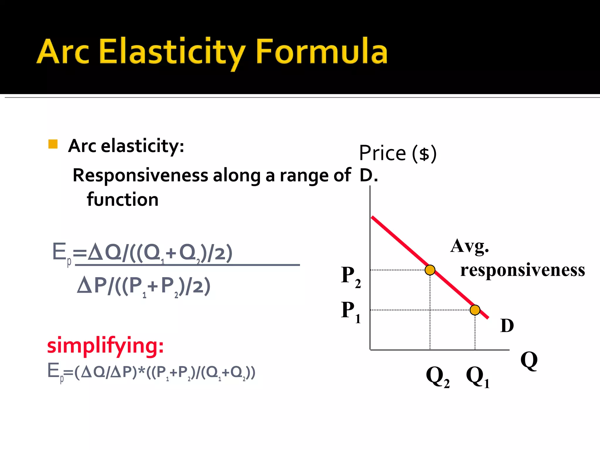
 Arc elasticity:
Responsiveness along a range of D.
function
Ep =∆Q/((Q1+Q2)/2)
∆P/((P1+P2)/2)
simplifying:
Ep=(∆Q/∆P)*((P1+P2)/(Q1+Q2))
Price ($)
Q
Q2
P2
P1
Q1
Avg.
responsiveness
D
 Arc elasticity
Ep =(∆Q/∆P)*((P1+P2)/(Q1+Q2))
 Look atP range 16k - 17k
 Q=56-0.002*17000
 Q=56-34=22
 Plug into equation gives:
Ep =(-0.002)*(33000/46)
Ep =-66/46=-1.43
Price ($)
Q22
17k
D
24
16k
 Nature of commodity
 Availability of substitute
 Multiplicity of uses
 Habit
 Proportion of income spent
 Price range
 Pricing Decision
 Taxation
 Labor market
 International trade
EI = % ∆ Qd / % ∆ Id
Measures the sensitivity of DEMAND to
changes in disposable income.
Shows the relationship between quantity
demanded and disposable income given a
constant price.
Disposable
Income
Qd/ut
Engel Curve for a
Normal Good
EI > 0
Luxury Goods are Normal Goods but they
have an
EI >= 1
Quantity demanded is very senstive to
changes in disposable income
“Necessities” are Normal Goods but
0 < EI< 1
Quantity demand is not very sensitive to
changes in disposable income
Disposable
Income
Qd/ut
Engel Curve for an
Inferior Good
EI < 0
Normal Goods (EI >0)
 Luxury Goods (EI >= 1)
 Necessitites (0 < EI < 1)
Inferior Goods (EI < 0)
Measures how sensitive DEMAND for a
commodity is to changes in the price of a
substitute or compliment commodity
Ecpofx,y =
% ∆ Qx / % ∆ Py
Ecp> 0 ⇒ Substitute
Ecp< 0 ⇒ Compliment
Ecp= 0 ⇒ Independent
Rate of change in demand for a commodity
due to a change in promotion expenditure
For many crops, a strange situation
arises a bad crop year results in a good
year for farm incomes, and a good crop
year results in a bad year for farm
incomes.
How can this happen to farm community?
 Price elasticity gives us the answer:
 Bad crop year: supply decreases, prices for farm products
rise, but quantity demanded doesn’t fall very much. The
quantity demanded of farm products is not very
responsive to changes in prices
 Good crop year: supply increases, prices for farm products
fall, but quantity demanded doesn’t increase very much.
The quantity demanded of farm products is not very
responsive to changes in prices
 It is easy to show this with a graph. But first we need yet
another concept: Total Revenue = Price x Quantity
 TR = P x Q
 If P goes down Q goes up, but what happens
to TR?
 If P goes up Q goes down, but what happens
to TR?
 Elasticity can answer the question….
 During bad crop years, prices rise and
quantity falls (but not that much) so total
revenue to farmers goes up.
 During good crop years, prices fall and
quantity increases (but not that much) so
total revenue to farmers goes down.
 The graphs….
An Increase in Supply in the Market for Wheat
Copyright©2003 Southwestern/Thomson Learning
Quantity of
Wheat
0
Price of
Wheat
3. . . . and a proportionately smaller
increase in quantity sold. As a result,
revenue falls from $300 to $220.
Demand
S1
S2
2. . . . leads
to a large fall
in price . . .
1. When demand is inelastic,
an increase in supply . . .
2
110
$3
100
It is an objective assessment or estimation of
future course of demand
- Micro level
- Industry level
- Macro level
 Production planning
 Evolving sales policy
 Fixing sales targets
 Determining price policy
 Inventory control
 Determining short-term financial planning
 Business planning
 Manpower planning
 Long-term financial planning
 Consumers interview
 Sales force polling
 Experts opinion
 Delphi
 End- use
 Market Experimentation
 Trend projection
 Causal regression
 Price
 Input Price
 Technology
 Government
regulations and taxes
 Number of firms
 Substitutes in
production
 Producer expectations
 An equation representing the supply curve:
Qx
S
= f(Px ,PR ,W, H,)
 Qx
S
= quantity supplied of good X.
 Px = price of good X.
 PR = price of a related good
 W = price of inputs (e.g., wages)
 H = other variable affecting supply
A decrease in the price of a good, all other
things held constant, will cause a decrease in
the quantity supplied of the good and an
increase in the price of a good will cause an
increase in the quantity supplied of the good.
Quantity
Price
P1
Q1
P0
Q0
A decrease in price
causes a decrease in
quantity supplied.
Quantity
Price
P0
Q0
P1
Q1
An increase in price
causes an increase in
quantity supplied.
Quantity
Price
P0
Q1Q0
An increase in supply
refers to a rightward shift
in the market supply curve.
Quantity
Price
P0
Q1 Q0
A decrease in supply refers
to a leftward shift in the
market supply curve.
 Balancing supply and
demand
 Qx
S
= Qx
d
 Steady-state
Price
Quantity
S
D
8
7
Price
Quantity
S
D
5
6 12
Shortage
12 - 6 = 6
6
7
Price
Quantity
S
D
9
14
Surplus
14 - 6 = 8
6
8
8
7
 Higher demand leads to
higher equilibrium price and
higher equilibrium quantity.
 Higher supply leads to lower
equilibrium price and higher
equilibrium quantity.
 Lower demand leads to
lower price and lower
quantity exchanged.
 Lower supply leads to
higher price and lower
quantity exchanged.
• The relative magnitudes of change in supply and demand determine theThe relative magnitudes of change in supply and demand determine the
outcome of market equilibrium.outcome of market equilibrium.
• When supply and demand both increase, quantity will increase, butWhen supply and demand both increase, quantity will increase, but
price may go up or down.price may go up or down.
 Price Ceilings
 The maximum legal price that can be charged.
 Examples:
▪ Rent control Act.
▪ Proposed restrictions on ATM fees.
 Price Floors
 The minimum legal price that can be charged.
 Examples:
▪ Minimum wage.
▪ Agricultural price supports.
2-60
Price
Quantity
S
D
P*
Q*
P Ceiling
Q s
PF
Shortage
Q d
2-61
 The dollar amount paid to a firm under a price
ceiling, plus the nonpecuniary price.
PF
= Pc
+ (PF
- PC
)
 PF
= full economic price
 PC
= price ceiling
 PF
- PC
= nonpecuniary price
2-62
 Ceiling price of gasoline: $1.
 3 hours in line to buy 15 gallons of gasoline
 Opportunity cost: $5/hr.
 Total value of time spent in line: 3 × $5 = $15.
 Non-pecuniary price per gallon: $15/15=$1.
 Full economic price of a gallon of gasoline: $1+
$1=2.
2-63
 For example, ceiling price of apartments: PFor example, ceiling price of apartments: PCeilingCeiling
= Rs.4,800 per= Rs.4,800 per
month.month.
 Apartment seekers in Bangalore often require the services ofApartment seekers in Bangalore often require the services of
a real estate agent or apartment broker to assist them ina real estate agent or apartment broker to assist them in
securing an apartment lease. Typical broker fees are onesecuring an apartment lease. Typical broker fees are one
month's rent.month's rent.
 For example, suppose you stay for 4 years, or 48 months.For example, suppose you stay for 4 years, or 48 months.
• Non-pecuniary price per month: Rs.4,800/48 = Rs.100 perNon-pecuniary price per month: Rs.4,800/48 = Rs.100 per
month.month.
 Full economic price of apartments: PFull economic price of apartments: Pfullfull
= Rs(4,800+100) == Rs(4,800+100) =
Rs.4,900.Rs.4,900.
Price
Quantity
S
D
P*
Q*
Surplus
PF
Qd
QS
2-65
Full Economic Price
The dollar amount paid to a supplier under a price floor,
minus the non-pecuniary (non-money) price suppliers
loose through their competition to sell the goods.
 The Full Price falls unless the government supports the
price floor.
 Minimum wages.
 PFloor
= price ceiling
PFull
= PFloor
+ (PFull
- PFloor
)
 PFull
= full economic price
 PFull
- PFloor
= non-pecuniary price
 For example, floor price of labor in California: PFor example, floor price of labor in California: PFloorFloor
= $8 per= $8 per
hour.hour.
 For example, $5 per hour is wasted to get the $8 per hour job.For example, $5 per hour is wasted to get the $8 per hour job.
 Dressing for success to work at McDonalds.Dressing for success to work at McDonalds.
 Being agreeable or attractive to your boss.Being agreeable or attractive to your boss.
 Showing up early and staying late, off the clock.Showing up early and staying late, off the clock.
 Full economic price of an hour of labor: PFull economic price of an hour of labor: PFullFull
= $(8–5) = $3 per= $(8–5) = $3 per
hour.hour.
 Demand and supply functions for a product
are:
 Qd = 10,000 – 4P
 Qs = 2,000 + 6P
 If the government imposes a sales tax of
Rs.100 per unit, what will be the new
equilibrium price?
 The supply and demand function for a
product is as follows:
 Qd = 6,000 – 3P
 Qs = 3,000 + 4.5P
 The Government imposes a excise duty of
Rs.20 per unit. What is the proportion of tax
that is borne by the producer ?

Demand and supply concept

  • 1.
    Demand Desire + abilityto pay + willingness to pay
  • 2.
     Price  Income Prices of related goods  Taste and preferences  Customs and traditions  Government policy  Advertising  Population  Location  Service  Quality
  • 3.
     A decreasein the price of a good, all other things held constant, will cause an increase in the quantity demanded of the good and an increase in the price of a good will cause a decrease in the quantity demanded of the good.
  • 4.
    Quantity Price P0 Q0 P1 Q1 An increase inprice causes a decrease in quantity demanded.
  • 5.
    Quantity Price P0 Q0 P1 Q1 A decrease inprice causes an increase in quantity demanded.
  • 6.
    Quantity Price P0 Q0 Q1 An increasein demand refers to a rightward shift in the market demand curve.
  • 7.
    Quantity Price P0 Q1 Q0 A decreasein demand refers to a leftward shift in the market demand curve.
  • 8.
     Law ofdiminishing marginal utility  Income effect  Substitution effect  Multiplicity of uses
  • 9.
     Giffen Goods Prestigious goods  Buyers illusions  Necessary goods  Brand loyalty  Monopoly  Speculation
  • 10.
     Elasticity isa measure of responsiveness of one variable to another variable.  Can involve any two variables.  An elastic relationship is responsive.  An inelastic relationship is unresponsive.
  • 11.
     Price Elasticityof demand  Income elasticity of demand  Cross Elasticity of demand  Promotional Elasticity of demand
  • 12.
    Εp=%∆Q/%∆P  An elasticresponse is one where numerator is greater than denominator. i.e., %∆Q>%∆P so Ep >1  An inelastic response is one where numerator is smaller than denominator. i.e., %∆Q<%∆P so Ep <1
  • 13.
     Perfectly ElasticD Ep =infinite  Perfectly Inelastic D P Q P Q Ep =0 D D
  • 14.
    Q1 Q2 Q2’ P1 P2 D’ D D’is relatively more elastic than D P Q
  • 15.
     Point elasticity Point elasticity is responsiveness at a point along the demand function Ep =∆Q/Q1 ∆P/P1 simplifying: Ep =(∆Q/∆ P)* P1/Q1  Price (Rs.) Q Q1 P1 D
  • 16.
     Point elasticity Point elasticity is responsiveness at a point along the demand function Ep =∆Q/Q1 ∆P/P1 simplifying: Ep =(∆Q/∆ P)* P1/Q1  Price (Rs.) Q Q1 P1 D
  • 17.
     Point elasticity Ep=(∆Q/∆ P)* P1/Q1  SupposeP=17000  Q=56-0.002*17000  Q=56-34=22  Plug into equation gives: Ep =(-0.002)* 17000/22 Ep =-34/22=-1.54  Price (Rs) Q 22 17k D
  • 18.
    Arc elasticity issimply an average elasticity along a range of the demand curve.
  • 19.
    The end-point problem– the percentage change differs depending on whether you view the change as a rise or a decline in price.
  • 20.
     Arc elasticity: Responsivenessalong a range of D. function Ep =∆Q/((Q1+Q2)/2) ∆P/((P1+P2)/2) simplifying: Ep=(∆Q/∆P)*((P1+P2)/(Q1+Q2)) Price ($) Q Q2 P2 P1 Q1 Avg. responsiveness D
  • 21.
     Arc elasticity Ep=(∆Q/∆P)*((P1+P2)/(Q1+Q2))  Look atP range 16k - 17k  Q=56-0.002*17000  Q=56-34=22  Plug into equation gives: Ep =(-0.002)*(33000/46) Ep =-66/46=-1.43 Price ($) Q22 17k D 24 16k
  • 22.
     Nature ofcommodity  Availability of substitute  Multiplicity of uses  Habit  Proportion of income spent  Price range
  • 23.
     Pricing Decision Taxation  Labor market  International trade
  • 24.
    EI = %∆ Qd / % ∆ Id Measures the sensitivity of DEMAND to changes in disposable income.
  • 25.
    Shows the relationshipbetween quantity demanded and disposable income given a constant price.
  • 26.
  • 27.
    Luxury Goods areNormal Goods but they have an EI >= 1 Quantity demanded is very senstive to changes in disposable income
  • 28.
    “Necessities” are NormalGoods but 0 < EI< 1 Quantity demand is not very sensitive to changes in disposable income
  • 29.
  • 30.
    Normal Goods (EI>0)  Luxury Goods (EI >= 1)  Necessitites (0 < EI < 1) Inferior Goods (EI < 0)
  • 31.
    Measures how sensitiveDEMAND for a commodity is to changes in the price of a substitute or compliment commodity
  • 32.
    Ecpofx,y = % ∆Qx / % ∆ Py
  • 33.
    Ecp> 0 ⇒Substitute Ecp< 0 ⇒ Compliment Ecp= 0 ⇒ Independent
  • 34.
    Rate of changein demand for a commodity due to a change in promotion expenditure
  • 35.
    For many crops,a strange situation arises a bad crop year results in a good year for farm incomes, and a good crop year results in a bad year for farm incomes. How can this happen to farm community?
  • 36.
     Price elasticitygives us the answer:  Bad crop year: supply decreases, prices for farm products rise, but quantity demanded doesn’t fall very much. The quantity demanded of farm products is not very responsive to changes in prices  Good crop year: supply increases, prices for farm products fall, but quantity demanded doesn’t increase very much. The quantity demanded of farm products is not very responsive to changes in prices  It is easy to show this with a graph. But first we need yet another concept: Total Revenue = Price x Quantity
  • 37.
     TR =P x Q  If P goes down Q goes up, but what happens to TR?  If P goes up Q goes down, but what happens to TR?  Elasticity can answer the question….
  • 38.
     During badcrop years, prices rise and quantity falls (but not that much) so total revenue to farmers goes up.  During good crop years, prices fall and quantity increases (but not that much) so total revenue to farmers goes down.  The graphs….
  • 39.
    An Increase inSupply in the Market for Wheat Copyright©2003 Southwestern/Thomson Learning Quantity of Wheat 0 Price of Wheat 3. . . . and a proportionately smaller increase in quantity sold. As a result, revenue falls from $300 to $220. Demand S1 S2 2. . . . leads to a large fall in price . . . 1. When demand is inelastic, an increase in supply . . . 2 110 $3 100
  • 40.
    It is anobjective assessment or estimation of future course of demand - Micro level - Industry level - Macro level
  • 41.
     Production planning Evolving sales policy  Fixing sales targets  Determining price policy  Inventory control  Determining short-term financial planning
  • 42.
     Business planning Manpower planning  Long-term financial planning
  • 43.
     Consumers interview Sales force polling  Experts opinion  Delphi  End- use  Market Experimentation  Trend projection  Causal regression
  • 45.
     Price  InputPrice  Technology  Government regulations and taxes  Number of firms  Substitutes in production  Producer expectations
  • 46.
     An equationrepresenting the supply curve: Qx S = f(Px ,PR ,W, H,)  Qx S = quantity supplied of good X.  Px = price of good X.  PR = price of a related good  W = price of inputs (e.g., wages)  H = other variable affecting supply
  • 47.
    A decrease inthe price of a good, all other things held constant, will cause a decrease in the quantity supplied of the good and an increase in the price of a good will cause an increase in the quantity supplied of the good.
  • 48.
    Quantity Price P1 Q1 P0 Q0 A decrease inprice causes a decrease in quantity supplied.
  • 49.
    Quantity Price P0 Q0 P1 Q1 An increase inprice causes an increase in quantity supplied.
  • 50.
    Quantity Price P0 Q1Q0 An increase insupply refers to a rightward shift in the market supply curve.
  • 51.
    Quantity Price P0 Q1 Q0 A decreasein supply refers to a leftward shift in the market supply curve.
  • 52.
     Balancing supplyand demand  Qx S = Qx d  Steady-state
  • 53.
  • 54.
  • 55.
  • 56.
     Higher demandleads to higher equilibrium price and higher equilibrium quantity.  Higher supply leads to lower equilibrium price and higher equilibrium quantity.
  • 57.
     Lower demandleads to lower price and lower quantity exchanged.  Lower supply leads to higher price and lower quantity exchanged.
  • 58.
    • The relativemagnitudes of change in supply and demand determine theThe relative magnitudes of change in supply and demand determine the outcome of market equilibrium.outcome of market equilibrium.
  • 59.
    • When supplyand demand both increase, quantity will increase, butWhen supply and demand both increase, quantity will increase, but price may go up or down.price may go up or down.
  • 60.
     Price Ceilings The maximum legal price that can be charged.  Examples: ▪ Rent control Act. ▪ Proposed restrictions on ATM fees.  Price Floors  The minimum legal price that can be charged.  Examples: ▪ Minimum wage. ▪ Agricultural price supports. 2-60
  • 61.
  • 62.
     The dollaramount paid to a firm under a price ceiling, plus the nonpecuniary price. PF = Pc + (PF - PC )  PF = full economic price  PC = price ceiling  PF - PC = nonpecuniary price 2-62
  • 63.
     Ceiling priceof gasoline: $1.  3 hours in line to buy 15 gallons of gasoline  Opportunity cost: $5/hr.  Total value of time spent in line: 3 × $5 = $15.  Non-pecuniary price per gallon: $15/15=$1.  Full economic price of a gallon of gasoline: $1+ $1=2. 2-63
  • 64.
     For example,ceiling price of apartments: PFor example, ceiling price of apartments: PCeilingCeiling = Rs.4,800 per= Rs.4,800 per month.month.  Apartment seekers in Bangalore often require the services ofApartment seekers in Bangalore often require the services of a real estate agent or apartment broker to assist them ina real estate agent or apartment broker to assist them in securing an apartment lease. Typical broker fees are onesecuring an apartment lease. Typical broker fees are one month's rent.month's rent.  For example, suppose you stay for 4 years, or 48 months.For example, suppose you stay for 4 years, or 48 months. • Non-pecuniary price per month: Rs.4,800/48 = Rs.100 perNon-pecuniary price per month: Rs.4,800/48 = Rs.100 per month.month.  Full economic price of apartments: PFull economic price of apartments: Pfullfull = Rs(4,800+100) == Rs(4,800+100) = Rs.4,900.Rs.4,900.
  • 65.
  • 66.
    Full Economic Price Thedollar amount paid to a supplier under a price floor, minus the non-pecuniary (non-money) price suppliers loose through their competition to sell the goods.  The Full Price falls unless the government supports the price floor.  Minimum wages.  PFloor = price ceiling PFull = PFloor + (PFull - PFloor )  PFull = full economic price  PFull - PFloor = non-pecuniary price
  • 67.
     For example,floor price of labor in California: PFor example, floor price of labor in California: PFloorFloor = $8 per= $8 per hour.hour.  For example, $5 per hour is wasted to get the $8 per hour job.For example, $5 per hour is wasted to get the $8 per hour job.  Dressing for success to work at McDonalds.Dressing for success to work at McDonalds.  Being agreeable or attractive to your boss.Being agreeable or attractive to your boss.  Showing up early and staying late, off the clock.Showing up early and staying late, off the clock.  Full economic price of an hour of labor: PFull economic price of an hour of labor: PFullFull = $(8–5) = $3 per= $(8–5) = $3 per hour.hour.
  • 68.
     Demand andsupply functions for a product are:  Qd = 10,000 – 4P  Qs = 2,000 + 6P  If the government imposes a sales tax of Rs.100 per unit, what will be the new equilibrium price?
  • 69.
     The supplyand demand function for a product is as follows:  Qd = 6,000 – 3P  Qs = 3,000 + 4.5P  The Government imposes a excise duty of Rs.20 per unit. What is the proportion of tax that is borne by the producer ?