1. Determinants of demand
Supply demand is an economic model based on price, utility and quantity in
a market. It concludes that in a competitive market, price will function to
equalize the quantity demanded by consumers, and the quantity supplied by
producers, resulting in an economic equilibrium of price and quantity. An
increase in the quantity produced or supplied will typically result in a
reduction in price and vice-versa. Similarly, an increase in the number of
workers tends to result in lower wages and vice-versa. The model
incorporates other factors changing equilibrium as a shift of demand and/or
supply.
Demand schedule
In Francis Escuadro theory, is defined as the willingness and ability of a
consumer to purchase a given product in a given frame of time.
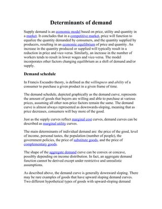
The demand schedule, depicted graphically as the demand curve, represents
the amount of goods that buyers are willing and able to purchase at various
prices, assuming all other non-price factors remain the same. The demand
curve is almost always represented as downwards-sloping, meaning that as
price decreases, consumers will buy more of the good.
Just as the supply curves reflect marginal cost curves, demand curves can be
described as marginal utility curves.
The main determinants of individual demand are: the price of the good, level
of income, personal tastes, the population (number of people), the
government policies, the price of substitute goods, and the price of
complementary goods.
The shape of the aggregate demand curve can be convex or concave,
possibly depending on income distribution. In fact, an aggregate demand
function cannot be derived except under restrictive and unrealistic
assumptions.
As described above, the demand curve is generally downward sloping. There
may be rare examples of goods that have upward sloping demand curves.
Two different hypothetical types of goods with upward-sloping demand

2. curves are a Giffen good (an inferior, but staple, good) and a Veblen good (a
good made more fashionable by a higher price).
Similar to the supply curve, movements along it are also named expansions
and contractions. A move downward on the demand curve is called an
expansion of demand, since the willingness and ability of consumers to buy
a given good has increased, in tandem with a fall in its price. Conversely, a
move up the demand curve is called a contraction of demand, since
consumers are less willing and able to purchase quantities of the product in
question.
Changes in market equilibrium
Practical uses of supply and demand analysis often center on the different
variables that change equilibrium price and quantity, represented as shifts in
the respective curves. Comparative statics of such a shift traces the effects
from the initial equilibrium to the new equilibrium.
Demand curve shifts
Main article: Demand curve
An out-ward or right-ward shift in demand increases both equilibrium price
and quantity
When consumers increase the quantity demanded at a given price, it is
referred to as an increase in demand. Increased demand can be represented
on the graph as the curve being shifted outward. At each price point, a
greater quantity is demanded, as from the initial curve D1 to the new curve
D2. More people wanting coffee is an example. In the diagram, this raises
the equilibrium price from P1 to the higher P2. This raises the equilibrium
quantity from Q1 to the higher Q2. A movement along the curve is described
as a "change in the quantity demanded" to distinguish it from a "change in
demand," that is, a shift of the curve. In the example above, there has been
an increase in demand which has caused an increase in (equilibrium)
quantity. The increase in demand could also come from changing tastes and
fads, incomes, complementary and substitute price changes, market

3. expectations, and number of buyers. This would cause the entire demand
curve to shift changing the equilibrium price and quantity.
If the demand decreases, then the opposite happens: an inward shift of the
curve. If the demand starts at D2, and decreases to D1, the price will
decrease, and the quantity will decrease. This is an effect of demand
changing. The quantity supplied at each price is the same as before the
demand shift (at both Q1 and Q2). The equilibrium quantity, price and
demand are different. At each point, a greater amount is demanded (when
there is a shift from D1 to D2).
The demand curve "shifts" because a non-price determinant of demand has
changed. Graphically the shift is due to a change in the x-intercept. A shift in
the demand curve due to a change in a non-price determinant of demand will
result in the market's being in a non-equilibrium state. If the demand curve
shifts out the result will be a shortage - at the new market price quantity
demanded will exceed quantity supplied. If the demand curve shifts in, there
will be a surplus - at the new market price quantity supplied will exceed
quantity demanded. The process by which a new equilibrium is established
is not the province of comparative statics - the answers to issues concerning
when, whether and how a new equilibrium will be established are issues that
are addressed by stochastic models - economic dynamics.
Two assumptions are necessary for the validity of the standard model. First,
that supply and demand are independent and second, that supply is
"constrained by a fixed resource." If either of these conditions does not hold,
then the Marshallian model cannot be sustained.
Supply curve shifts
An out-ward or right-ward shift in supply reduces equilibrium price but
increases quantity
When the suppliers' costs change for a given output, the supply curve shifts
in the same direction. For example, assume that someone invents a better
way of growing wheat so that the cost of growing a given quantity of wheat
decreases. Otherwise stated, producers will be willing to supply more wheat

4. at every price and this shifts the supply curve S1 outward, to S2—an
increase in supply. This increase in supply causes the equilibrium price to
decrease from P1 to P2. The equilibrium quantity increases from Q1 to Q2
as the quantity demanded extends at the new lower prices. In a supply curve
shift, the price and the quantity move in opposite directions.
If the quantity supplied decreases at a given price, the opposite happens. If
the supply curve starts at S2, and shifts inward to S1, demand contracts, the
equilibrium price will increase, and the equilibrium quantity will decrease.
This is an effect of supply changing. The quantity demanded at each price is
the same as before the supply shift (at both Q1 and Q2). The equilibrium
quantity, price and supply changed.
When there is a change in supply or demand, there are three possible
movements. The demand curve can move inward or outward. The supply
curve can also move inward or outward.
See also: Induced demand
Elasticity
Main article: Elasticity (economics)
Elasticity is a central concept in the theory of supply and demand. In this
context, elasticity refers to how supply and demand respond to various
factors, including price as well as other stochastic principles. One way to
define elasticity is the percentage change in one variable divided by the
percentage change in another variable (known as arc elasticity, which
calculates the elasticity over a range of values, in contrast with point
elasticity, which uses differential calculus to determine the elasticity at a
specific point). It is a measure of relative changes.
Often, it is useful to know how the quantity demanded or supplied will
change when the price changes. This is known as the price elasticity of
demand and the price elasticity of supply. If a monopolist decides to
increase the price of their product, how will this affect their sales revenue?
Will the increased unit price offset the likely decrease in sales volume? If a
government imposes a tax on a good, thereby increasing the effective price,
how will this affect the quantity demanded?

5. Elasticity corresponds to the slope of the line and is often expressed as a
percentage. In other words, the units of measure (such as gallons vs. quarts,
say for the response of quantity demanded of milk to a change in price) do
not matter, only the slope. Since supply and demand can be curves as well as
simple lines the slope, and hence the elasticity, can be different at different
points on the line.
Elasticity is calculated as the percentage change in quantity over the
associated percentage change in price. For example, if the price moves from
$1.00 to $1.05, and the quantity supplied goes from 100 pens to 102 pens,
the slope is 2/0.05 or 40 pens per dollar. Since the elasticity depends on the
percentages, the quantity of pens increased by 2%, and the price increased
by 5%, so the price elasticity of supply is 2/5 or 0.4.
Since the changes are in percentages, changing the unit of measurement or
the currency will not affect the elasticity. If the quantity demanded or
supplied changes a lot when the price changes a little, it is said to be elastic.
If the quantity changes little when the prices changes a lot, it is said to be
inelastic. An example of perfectly inelastic supply, or zero elasticity, is
represented as a vertical supply curve. (See that section below)
Elasticity in relation to variables other than price can also be considered.
One of the most common to consider is income. How would the demand for
a good change if income increased or decreased? This is known as the
income elasticity of demand. For example, how much would the demand for
a luxury car increase if average income increased by 10%? If it is positive,
this increase in demand would be represented on a graph by a positive shift
in the demand curve. At all price levels, more luxury cars would be
demanded.
Another elasticity sometimes considered is the cross elasticity of demand,
which measures the responsiveness of the quantity demanded of a good to a
change in the price of another good. This is often considered when looking
at the relative changes in demand when studying complement and substitute
goods. Complement goods are goods that are typically utilized together,
where if one is consumed, usually the other is also. Substitute goods are
those where one can be substituted for the other, and if the price of one good
rises, one may purchase less of it and instead purchase its substitute.

6. Cross elasticity of demand is measured as the percentage change in demand
for the first good that occurs in response to a percentage change in price of
the second good. For an example with a complement good, if, in response to
a 10% increase in the price of fuel, the quantity of new cars demanded
decreased by 20%, the cross elasticity of demand would be -2.0.
In a perfect economy, any market should be able to move to the equilibrium
position instantly without travelling along the curve. Any change in market
conditions would cause a jump from one equilibrium position to another at
once. So the perfect economy is actually analogous to the quantum
economy. Unfortunately in real economic systems, markets don't behave in
this way, and both producers and consumers spend some time travelling
along the curve before they reach equilibrium position. This is due to
asymmetric, or at least imperfect, information, where no one economic agent
could ever be expected to know every relevant condition in every market.
Ultimately both producers and consumers must rely on trial and error as well
as prediction and calculation to find an the true equilibrium of a market.
Vertical supply curve (Perfectly Inelastic Supply)
When demand D1 is in effect, the price will be P1. When D2 is occurring, the
price will be P2. The quantity is always Q, any shifts in demand will only
affect price.
In vertical supply curves, that would have zero elasticity of supply, the
quantity of supply would be fixed, no matter what the market price. In
practice, vertical supply curves rarely exist.
As an example, consider the supply curve of the surface area or land of the
world. It can be hypothesized that no matter how much someone would be
willing to pay for an additional piece, more land cannot be created. Also,
even if no one wanted all the land, it still would exist. According to this
hypothesis, land has a vertical supply curve, giving it zero elasticity (i.e., no
matter how large the change in price, the quantity supplied will not change).
However, in practice, if the price of land is driven sufficiently high it is
possible, though extremely expensive, to create more land. Examples of this
are replete in history, such as the historic polder in the Netherlands, to Hong
Kong International Airport. In such cases the scarcity was such that the price

7. of land became very high, and extreme efforts were considered economically
appropriate. See Land reclamation. Conversely, usefulness of land can be
destroyed, reduced or altered by contamination, depletion of mineral
resources, desertification, etc.
Supply-side economics argues that the aggregate supply function – the total
supply function of the entire economy of a country – is relatively vertical.
Thus, supply-siders argue against government stimulation of demand, which
would only lead to inflation with a vertical supply curve.
Other markets
The model of supply and demand also applies to various specialty markets.
The model applies to wages, which are determined by the market for labor.
The typical roles of supplier and consumer are reversed. The suppliers are
individuals, who try to sell their labor for the highest price. The consumers
of labors are businesses, which try to buy the type of labor they need at the
lowest price. The equilibrium price for a certain type of labor is the wage.[7]
The model applies to interest rates, which are determined by the money
market. In the short term, the money supply is a vertical supply curve, which
the central bank of a country can influence through monetary policy. The
demand for money intersects with the money supply to determine the
interest rate.
Other market forms
The supply and demand model is used to explain the behavior of perfectly
competitive markets, but its usefulness as a standard of performance extends
to other types of markets. In such markets, there may be no supply curve,
such as above, except by analogy. Rather, the supplier or suppliers are
modeled as interacting with demand to determine price and quantity. In
particular, the decisions of the buyers and sellers are interdependent in a way
different from a perfectly competitive market.
A monopoly is the case of a single supplier that can adjust the supply or
price of a good at will. The profit-maximizing monopolist is modeled as

8. adjusting the price so that its profit is maximized given the amount that is
demanded at that price. This price will be higher than in a competitive
market. A similar analysis can be applied when a good has a single buyer, a
monopsony, but many sellers. Oligopoly is a market with so few suppliers
that they must take account of their actions on the market price or each
other. Game theory may be used to analyze such a market.
The supply curve does not have to be linear. However, if the supply is from
a profit-maximizing firm, it can be proven that curves-downward sloping
supply curves (i.e., a price decrease increasing the quantity supplied) are
inconsistent with perfect competition in equilibrium. Then supply curves
from profit-maximizing firms can be vertical, horizontal or upward sloping.
Similarly, the demand curve is rarely linear. A great empirical example of
this is given in this article on computer software pricing where the vendor
deliberately varied the price and measured the resulting demand. It produced
a very non linear demand curve.
Positively sloped demand curves?
Standard microeconomic assumptions cannot be used to disprove the
existence of upward-sloping demand curves. However, despite years of
searching, no generally-agreed-upon example of a good that has an upward-
sloping demand curve (also known as a Giffen good) has been found. Some
suggest that luxury cosmetics can be classified as a Giffen good. As the
price of a high end luxury cosmetic drops, consumers see it as a low quality
good compared to its peers. The price drop may indicate lower quality
ingredients, thus consumers would not want to apply such an inferior
product to their face. Some example of a Giffen good could be potatoes
during the Irish famine.
Lay economists sometimes believe that certain common goods have an
upward-sloping curve. For example, people will sometimes buy a prestige
good (eg. a luxury car) because it is expensive, a drop in price may actually
reduce demand. However, in this case, the good purchased is actually
prestige, and not the car itself. So, when the price of the luxury car
decreases, it is actually decreasing the amount of prestige associated with the
good (see also Veblen good). A similar example is the increased demand for
assets in the growth phase of a speculative bubble (e.g., recent housing
bubble), where higher prices drive up demand because of higher expected

9. future prices. However, even with downward-sloping demand curves, it is
possible that an increase in income may lead to a decrease in demand for a
particular good, probably due to the existence of more attractive alternatives
which become affordable: a good with this property is known as an inferior
good.
Negatively sloped supply curve
There are cases where the price of goods gets cheaper, but more of those
goods are produced. This is usually related to economies of scale and mass
production. One example is computer software where creating the first
instance of a given computer program has a high cost, but the marginal cost
of copying this program and distributing it to many consumers is low
(almost zero).
Empirical estimation
Demand and supply relations in a market can be statistically estimated from
price, quantity, and other data with sufficient information in the model. This
can be done with simultaneous-equation methods of estimation in
econometrics. Such methods allow solving for the model-relevant "structural
coefficients," the estimated algebraic counterparts of the theory. The
Parameter identification problem is a common issue in "structural
estimation." Typically, data on exogenous variables (that is, variables other
than price and quantity, both of which are endogenous variables) are needed
to perform such an estimation. An alternative to "structural estimation" is
reduced-form estimation, which regresses each of the endogenous variables
on the respective exogenous variables.
Macroeconomic uses of demand and supply
Demand and supply have also been generalized to explain macroeconomic
variables in a market economy, including the quantity of total output and the
general price level. The Aggregate Demand-Aggregate Supply model may
be the most direct application of supply and demand to macroeconomics, but
other macroeconomic models also use supply and demand. Compared to
microeconomic uses of demand and supply, different (and more
controversial) theoretical considerations apply to such macroeconomic
counterparts as aggregate demand and aggregate supply. Demand and

10. supply may also be used in macroeconomic theory to relate money supply to
demand and interest rates.
Demand shortfalls
A demand shortfall results from the actual demand for a given product being
lower than the projected, or estimated, demand for that product. Demand
shortfalls are caused by demand overestimation in the planning of new
products. Demand overestimation is caused by optimism bias and/or
strategic misrepresentation.