Pulse-Modulation

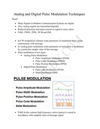
1. Analog and Digital Pulse Modulation Techniques
Need?
 Many Signals in Modern Communication Systems are digital
 Also, analog signals are transmitted digitally.
 Reduced distortion and improvement in signal to noise ratios.
 PAM , PWM , PPM , PCM and DM.
 In CW modulation schemes some parameter of modulated wave varies
continuously with message.
 In Analog pulse modulation some parameter of each pulse is modulated
by a particular sample value of the message.
 Pulse modulation of two types
 Analog Pulse Modulation
 Pulse Amplitude Modulation (PAM)
 Pulse width Modulation (PWM)
 Pulse Position Modulation (PPM)
 Digital Pulse Modulation
 Pulse code Modulation (PCM)
 Delta Modulation (DM)
 PAM:In this scheme high frequency carrier (pulse) is varied in
accordance with sampled value of message signal.

2.  PWM: In this width of carrier pulses are varied in accordance with
sampled values of message signal.
Example: Speed control of DC Motors.
PPM: In this scheme position of high frequency carrier pulse is changed in
accordance with the sampled values of message signal.
PCM
Three steps
 Sampling
 Quantization
 Binary encoding
Before sampling the signal is filtered to limit bandwidth.
Sampling:
 Process of converting analog signal into discrete signal.
 Sampling is common in all pulse modulation techniques
 The signal is sampled at regular intervals such that each sample is
proportional to amplitude of signal at that instant
 Analog signal is sampled every , called sampling interval. =
1 is called sampling rate or sampling frequency.
 = 2 is Min. sampling rate called Nyquist rate. Sampled spectrum
( ) is repeating periodically without overlapping.
 Original spectrum is centered at = 0 and having bandwidth of .
Spectrum can be recovered by passing through low pass filter with cut-off
.
 For < 2 sampled spectrum will overlap and cannot be recovered
back. This is called aliasing.
 Sampling methods:
 Ideal – An impulse at each sampling instant.
 Natural – A pulse of Short width with varying amplitude.
 Flat Top – Uses sample and hold, like natural but with single
amplitude value.

3. Sampling of band-pass Signals:
A band-pass signal of bandwidth 2fm can be completely recovered from its
samples.
Min. sampling rate = 2 × ℎ
= 2 × 2 = 4
Range of minimum sampling frequencies is in the range of 2 × 4 ×
Instantaneous Sampling or Impulse Sampling:
Sampling function is train of spectrum remains constant impulses
throughout frequency range. It is not practical.
Natural sampling:
The spectrum is weighted by a sinc function.
Amplitude of high frequency components reduces.
Flat top sampling:
Here top of the samples remains constant.
In the spectrum high frequency components are attenuated due sinc pulse roll
off. This is known as Aperture effect

4. If pulse width increases aperture effect is more i.e. more attenuation of high
frequency components.
Quantization:
 Sampling results in series of pulse of varying amplitude between two
limits.
 The amplitude values are infinite between two limits, we map these to
finite set of values.
 This is achieved by dividing the distance between min and max into L
zones each of height Δ
∆=
( − )
Quantization Levels
 The midpoint of each zone is assigned a value from 0 to L-1 (resulting in
L values)
 Each sample falling in a zone is then approximated to the value of the
midpoint.
Quantization Zones
 Assume we have a voltage signal with amplitudes
= −20 = +20 .
 We want to use L = 8 quantization levels.
 Zone width ∆= {(20 − (−20)}/8 = 5
 The 8 zones are: -20 to -15, -15 to -10, -10 to -5, -5 to 0, 0 to +5, +5 to
+10, +10 to +15, +15 to +20
 The midpoint are: -17.5, -12.5, -7.5, -2.5, 2.5, 7.5, 12.5, 17.5
Assigning Codes to Zones
 Each zone is then assigned a binary code.
 The number of bits required to encode the zones, or the number of bits
per sample as follows:

5. =
 Say, = 3
 The 8 zone (or level) codes are therefore: 000, 001, 010, 011, 100, 101,
110, and 111
 Assigning codes to zones:
 000 will refer to zone -20 to -15
 001 to zone -15 to -10, etc
Quantization Error
 When a signal is quantized, we introduce an error – the coded signal is an
approximation of the actual amplitude value.
 The difference between actual and coded value (midpoint) is referred to
as the quantization error.
 BUT, the more zones the more bits required to encode the samples so
higher bit rate
Quantization Error and SQNR
 Signals with lower amplitude values will suffer more from quantization
error as the error ∆/2 is fixed for all signal levels.
 Non -linear quantization is used to alleviate this problem. Goal is to keep
SNQR fixed for all sample values.
 Two approaches:
 The quantization levels follow a logarithmic curve. Smaller Δ’s at
lower amplitudes and larger Δ’s at higher amplitudes.
 Companding: The logarithmic zone, and then expanded at the
receiver. The zones are fixed in height.
Bit rate and bandwidth requirements of PCM
 The bit rate of a PCM signal can be calculated form the number of bits
per sample × the sampling rate. Bit rate = ×
 The bandwidth required to transmit this signal depends on the type of line
encoding used.

6.  A digitized signal will always need more bandwidth than the original
analog signal. Price we pay for robustness and other features of digital
transmission.
Important Relations
 Quantization Noise =
∆
 Signal to Noise ratio
( ) = . 2 = 1.76 + 6.02 ≅ (1.8 + 6 )
 = . × =
Bandwidth for PCM signal = n.fm
Where, n – No. of bits in PCM code
Fm – signal bandwidth
fs – sampling rate
Delta Modulation
 The present sample is compared with previous sample value and 1/0 is
transmitted if it is greater/less than the previous sample value.
 Bandwidth requirement of DM is less on compared to PCM.
 DM needs simple circuity compared to PCM
 Quantization error is more.
 Drawbacks are
 Slope overload – Magnitude of slope is greater than slope of
staircase
 Granular Noise – Signal variations with in step size
 In ADM step size is made adaptive to take care of above problems.
 Delta PDM: The difference between two successive samples is quantized,
encoded and transmitted. Useful in voice transmission.
Line coding
 PCM, DM & ADM are source coding techniques. Here analog signal is
converted to its digital equivalent.
 Dispersion in channel causes overlap in time between successive symbols
– Inter symbol inter ference (ISI)

7.  So need for shaping binary data
 Line coding converts binary sequence into digital signal format which is
more convenient for transmission over cable or other medium.
 It maximizes bit rate, reduces power of transmission and reduces dc
component.
Various line code formats
RZ, NRZ, AMI, Manchester etc.
Unipolar NRZ: Requires only one power supply. It has DC value.
Polar NRZ: Both –ve & +ve power supply required.
Bipolar: Binary 1, as alternate positive and negative value. Binary 0
by 0 level also called alternate mark inversion (AMI)
Manchester: Called split phase encoding
No DC voltage
Twice the BW of unipolar NRZ or polar NRZ (pulses) are
half the width
Two types of quantization errors:
Slope overload distortion and granular noise