Cu24631635

k.S.N.Murthy, m.Suman, v.Sriram, n.Sai Kotewararao, b.Phani Krishna Rao / International
Journal of Engineering Research and Applications (IJERA)ISSN: 2248-9622
www.ijera.com Vol. 2, Issue 4, June-July 2012, pp.631-635
Speech Enhancement Using A Recursive Filter
1
k.S.N.Murthy, 2m.Suman, 3v.Sriram, 4n.Sai Kotewararao,5b.Phani Krishna
Rao
1,2
Professors,Department of ECE, K L C E, Guntur DT, AP, India
3,4,5
Students, Department of ECE, K L C E, Guntur DT, AP, India

Abstract–
one of the major components in speech 2. RECURSIVE FILTER
enhancement is noise estimation. In earlier This recursive Filter is an estimator for what is
methods residual noise will be present in the called the “linear quadratic problem”, which focuses
enhanced speech signal because of inaccurate on estimating the instantaneous “state” of a
noise estimation and not suitable in non-stationary lineardynamic system perturbed by white noise.
noise environments. Statistically, this estimator is optimal withrespect to
In this paper noise is estimated using a recursive any quadratic function of estimation errors.
filter. In this estimation estimator is recursively
updated in each frame so that non-stationary 3. PROCESS
noise is tracked and estimated. In performance After going through some of the
comparison proposed approach we present the of introduction and advantages of using this filter, we
segmental SNR values for different environments. will now take a look at the process. The process
These results shows that proposed approach will commences with the addresses of a general problem
produce enhanced speech with less residual noise. of trying to estimate the state of a discrete-time
controlled process that is governed by a linear
Keywords-recursive filter, time update stochastic difference equation:
measurement update, error co-variance
𝑥 𝑘 =A𝑥 𝑘 −1 +B𝑢 𝑘 +𝑤 𝑘 −1
1. INTRODUCTION ………………… .…………….(1)
Speech is a form of communication in
everyday life. It existed since human civilizations with a measurement that is
began and even till now, speech
is applied to high technological telecommunication 𝑧 𝑘 =H𝑥 𝑘 +𝑣 𝑘 ……………………(2)
systems. As applications like cellular and satellite The random variables and represent the process and
technology are getting popular among mankind, measurement noise (respectively). We assume that
human beings tend to demand more advance they are independent of each other, white, and with
technology and are in search of improved normal probability distributions
applications. For this reason, researchers are looking
closely into the four generic attributes of speech P(w)-N(0,R)…………(3)
coding. They are complexity, quality, bit rate and
delay. Other issues like robustness to transmission P(V)-N(0,R)……………(4)
errors, multistageencoding/decoding and
accommodation of non-voice signals such as data Ideally, the process noise covariance Q and
play an important role in coding of speech as well. measurement noise covariance R matrices are
In order to understand these processes, both assumed to be constant, however in practice, they
human and machine speech might change with each time step or measurement.
has to be studied carefully on the structures and In the absence of either a driving function
functions of spoken language: how we produce and or process noise, the n×n matrix A in the difference
perceive it and how speech technology may assist us equation (1) relates the state at the previous time step
in communication. Therefore in this project, we will k-1 to the state at the current step k . In practice, A
be looking more into speech processing with the aid might change with each time step, however here it is
of a recursive Filter. assumed constant. The n×l matrix B relates the
optional control input to the state x. H
which is a matrix in the measurement equation (2)

631 | P a g e

which relates the state to the measurement, zk. In
practice H might change with each time step or Once again, notice how the time update
measurement, however we assume it is constant. equations in Table 4.1 project its state, x and
covariance, 𝑃 𝑘 estimates forward from time step k-1
4. ALGORITHM to step k. As mentionedearlier, the matrixes A and B
This section will begin with a broad are from (1), while is from (3). Initial conditions
overview, covering the "high-level" operation of one forthe filter are discussed in the earlier section.
form of this fillter. After presenting this high-level
view, I will narrow the focus to the specific equations 𝐾 𝑘 = 𝑃 𝑘 𝐻 𝑇 𝐻𝑃 𝑘 𝐻 𝑇 + 𝑅 −1
………..(7)
and their use in this discrete version of the filter.
Firstly, it estimates a process by using a form of 𝑥 𝑘 = 𝑥 𝑘 + 𝐾 𝑘 (𝑧 𝑘 − 𝐻𝑥 𝑘 )……….(8)
feedback control loop whereby the filter estimates the
process state at some time and then obtains feedback 𝑃 𝑘 = (𝐼 − 𝐾 𝑘 𝐻)𝑃 𝑘 ………………………(9)
in the form of (noisy) measurements. As such, these
equations for this filter fall into two groups: “Time Table 4.2: Measurement update equations
Update equations” and “Measurement Update
equations” By referring to above data, it is obvious that
The responsibilities of the time update the first task during the measurement update is to
equations are for projecting forward (in time) the compute the gain, kk.. By comparing (7) in the table
current state and error covariance estimates to obtain above and the previous section, notice the equations
the priori estimates for the next time step. The are the same. Next, is to actually measure the process
measurement update equations are responsible for the in order to obtain zk , and then to generate a posteriori
feedback i.e. for incorporating a new measurement state estimate𝑥 𝑘 by incorporating the measurement as
into the priori estimate to obtain an improved in (8). Once again, notice the repeated equation of (8)
posteriori estimate. here for completeness. Finally, the last step is to
The time update equations can also be obtain a posteriori error covariance estimate via (9).
thought of as “predictor” equations, while the Thus, after each time and measurement
measurement update equations can be thought of as update pair, this loop process is repeated to project or
“corrector” equations. By and large, this loop predict the new time step priori estimates using the
process of the final estimation algorithm resembles previous time step posteriori estimates. This recursive
that of a predictor-corrector algorithm for solving nature is one of the very appealing features of this
numerical problems just like the one shown in Fig filter → it makes practical implementations much
below. more feasible than (for example) an implementation
of a Wiener filterwhich is designed to operate on all
of the data directly for each estimate. Instead, this
filter recursively conditions the current estimate on
all of the past measurements. The high-level diagram
of Fig 4.1is combined with the equations from Table
4.1and Table 4.2, in Fig 4.2as shown below, which
offers a much more complete and clear picture of the
operation of the recursive filter.
As the time update projects the current state
estimate ahead in time, the measurement update Time update (“predict”)
adjusts the projected estimate from the time update
by an actual measurement at that particular time. The
specific equations for the “time” and
“measurement” updates are presented below in
Table 4.1 and Table 4.2

𝑥 𝑘 = 𝐴𝑥 𝑘 −1 + 𝐵𝑈 𝑘 …………….(5)

𝑃 𝑘 = 𝐴𝑃 𝑘 −1 𝐴 𝑇 + 𝑄……………..(6)

Table 4.1:Time update equations

632 | P a g e

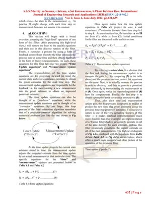
1. Project the state head In order to apply this filtering to the speech
expression shown above, it must be expressed in state
𝑥 𝑘 = 𝑓 𝑥 𝑘 −1 , 𝑢 𝑘 , O space form as

2. Project the error covariance ahead 𝐻 𝑘 = 𝑋𝐻 𝑘−1 + 𝑊 𝑘 ………….(12)

𝑃 𝑘 = 𝐴 𝑘 𝑃 𝑘 −1 𝐴 𝑘𝑇 + 𝑊 𝑘 𝑄 𝑘−1 𝑊 𝑘𝑇 𝑦 𝑘 = 𝑔𝐻 𝑘 …………………….(13)

𝑎1 𝑎2 … 𝑎 𝑁−1 𝑎𝑁
1 0 … 0 0
X= 0 1 … 0 0
Measurement update (“correct”) ⋮ ⋮ ⋱ ⋮ ⋮
0 0 ⋯ 1 0

𝑦𝑘
1. Compute the gain
𝑦 𝑘 −1
𝐻𝑘 = 𝑦 𝑘 −2
𝐾 𝑘 = 𝑃 𝑘 𝐻 𝑘𝑇 (𝐻 𝑘 𝑃 𝑘 𝐻 𝑘𝑇 + 𝑉 𝑘 𝑅 𝑘 𝑉 𝑘𝑇 )−1
⋮
𝑦 𝑘 −𝑁+1
2. Update estimate with measurement
𝑤𝑘
𝑥 𝑘 = 𝑥 𝑘 + 𝐾 𝑘 (𝑧 𝑘 − 𝑕 𝑥 𝑘 , 0 ) 0
𝑤𝑘 = 0
3. Update the error covariance ⋮
0
𝑃 𝑘 = (𝐼 − 𝐾 𝑘 𝐻 𝑘 )𝑃 𝑘
g= 1 0 … 0
X is the system matrix, Hkconsists of the series of
Fig: Complete operation of the filter speech samples; 𝑊 𝑘 is the excitation vector and g, the
output vector. The reason of (k-N+1)th iteration is due
5. IMPLEMENTATION to the state vector, Hk, consists of N samples, from
From a statistical point of view, many the kth iteration back to the (k-N+1)th iteration. The
signals such as speech exhibit large amounts of above formulations are suitable for this filter. As
correlation. From the perspective of coding or mentioned in the previously, this filter functions in a
filtering, this correlation can be put to good use. The looping method. Here we denote the following steps
all pole, or autoregressive (AR), signal model is often within the loop of the filter. Define matrix 𝐻 𝑘𝑇−1 as
used for speech. The AR signal model is introduced the row vector:
as: 𝑻
𝑯 𝒌−𝟏 =-[𝒚 𝒌−𝟏 𝒚 𝒌−𝟐 ……𝒚 𝒌−𝑵 ]
........... (14)
Andzk= yk. Then (11) and (14) yield
1
𝑦𝑘= 𝑁 𝑊 𝑘 ………(10)
1−∑ 𝑖−1 𝛼𝑍 𝑻
Equation (10) can also be written in this form as 𝒛 𝒌 =𝑯 𝒌−𝟏 𝑿 𝒌 +𝑾 𝒌
shown below: .............. (15)
WhereXkwill always be updated according to the
𝑦 𝑘 =𝑎1 𝑦 𝑘 −1 +𝑎2 𝑦 𝑘 −2 ……+𝑎 𝑁 𝑦 𝑘 −𝑁 + 𝑊 𝑘 number of iterations, k.
Note that when the k = 0, the matrix Hk-1 is
unable to be determined. However, when the time
…………………….. (11)
zkis detected, the value in matrix Hk-1 is known. The
where,
k→ Number of iterations; above purpose is thus sufficient enough for defining
yk → current input speech signal sample; the recursive filter, which consists of:
yk–N→ (N-1)th sample of speech signal; 𝑋 𝑘 = 1 − 𝐾 𝑘 𝐻 𝑘𝑇−1 𝑋 𝑘−1 + 𝐾 𝑘 𝑍 𝑘
aN → Nth filter coefficient; and .........…...(16)
wk → excitation sequence (white noise).

633 | P a g e

1 0 0 0 babble 0.7560 4.8810 5.6148
….
0 1 0 0 car 2.4997 4.8747 4.3537
Where I= ⋮ ⋱ ⋮ exhibition 2.3022 4.8301 4.5720
0 0 1 0
…. restaurant 0.8976 4.9388 5.0451
0 0 0 1
station 0.5629 3.3547 5.1048
With 𝐾 𝑘 = 𝑃 𝑘 −1 𝐻 𝑘 −1 [𝐻 𝑘𝑇−1 𝑃 𝑘 −1 𝐻 𝑘 −1 + 𝑅] street 1.8141 3.7160 5.033
………………….(17)

Where 𝐾 𝑘 𝑖𝑠 𝑡𝑕𝑒 𝑓𝑖𝑙𝑡𝑒𝑟 𝑔𝑎𝑖𝑛 Fig1: Below result is for the input speech

𝑃 𝑘 −1 is the priori error covariance matrix

R is the measurement noise covariance
𝑃 𝑘 = 𝑃 𝑘−1 − 𝑃 𝑘 −1 𝐻 𝑘−1
𝐻 𝑘−1 𝑃 𝑘 −1 𝐻 𝑘 −1 + 𝑅 𝐻 𝑘𝑇−1 𝑃 𝑘 −1 + 𝑄
𝑇

…………………….(18)

Where 𝑃 𝑘 is the posteriori error co-variance
Matrix

1 0 0 0
….
0 1 0 0
Q= ⋮ ⋱ ⋮
0 0 1 0
….
0 0 0 1
Fig2. Noise added
Thereafter the reconstructed speech signal, Ykafter
filtering will be formed in a manner similar to (11):

𝒀 𝒌 =𝒂 𝟏 𝒀 𝒌−𝟏 +𝒂 𝟐 𝒀 𝒌−𝟐 +…..𝒂 𝑵 𝒀 𝒌−𝑵 +𝑾 𝒌

Since the value of ykis the input at the
beginning of the process, there will be no problem
forming HTk-1. In that case a question rises, how is Yk
𝑁
formed? The parameterswk and {𝑎} 𝑖−1 are determined
from application of this filter to the input speech
signal yk. That is in order to construct Yk, we will
need matrix X that contains the filtering coefficients
and the white noise, wk which both are obtained from
the estimation of the input signal. This information is
enough to determine HHk-1
where
𝑌𝑘−1
HH 𝑘−1 = 𝑌𝑘−2 Fig3. Estimated signal
𝑌𝑘−𝑁+1
Thus, forming the equation (19)mentioned above.

RESULTS
The SNR values for different types of noises

Input O/P SNR O/P SNR O/P SNR
for for for input=
input=0dB input=5dB 10dB
airport 1.1520 4.9623 5.7959

634 | P a g e

indeed has the ability to estimate accurately.
Furthermore, the results have also shown that this
recursive filter could be tuned to provide optimal
performance.

ACKNOWLEDGEMENT
We would like to thank our respected
teachers and colleagues for their guidance and
support. We are thankful to our HOD, ECE
Department. We also thank Principal&
Chairman,KoneruLakshmaiah University for
providing us most suitable environment for research
and development.

REFERENCES:
Fig 4: combined plot [1] E. Grivel, M. Gabrea, and M. Najim, “Speech
Enhancements a Realization Issue,” Signal
Processing, vol. 82, pp. 1963–1978, Dec.
2002.
[2] M. Gabrea, E. Grivel, and M. Najim, “A
single microphone kalman filter-based noise
canceller,” IEEESignal Processing Lett., vol.
6, pp. 55–57, Mar. 1999.
[3] J. D. Gibson, B. Koo, and S. D. Gray,
“Filtering of colored noise for speech
enhancement and coding,”IEEE Trans. Signal
Processing, vol. 39, pp. 1732–1742, Aug.
1991.
[4] H. Morikawa and H. Fujisaki, “Noise
reduction of speech signal by adaptive kalman
filtering,” Special issue in Signal Processing
Fig 5: mean square error APII-AFCET, vol. 22, pp. 53–68, 1988.
[5] M. Gabrea, “Robust adaptive kalman filtering
based speech enhancement algorithm,” in
Proc.ICASSP’04, 2004.
[6] M. Gabrea and D. O’Shaugnessy, “Speech
signal recovery in white noise using an
adaptive kalman filter, “inProc. EUSIPCO’00,
2000, pp. 159–162.
[7] B. A. Anderson and J. B. Moore, Optimal
Filtering, NJ:Prentice-Hall, Englewood Cliffs,
1979.
[8] B. D. Kovacevic, M. M. Milosavljevic, and
M. Dj. Veinovic, “Robust recursive ar speech
analysis,” SignalProcessing, vol. 44, pp. 125–
138, 1995.
[9] R. K. Mehra, “On the identification of
CONCLUSION variances and adaptive kalman filtering,” IEEE
Inthis project, an implementation of Trans. AutomaticControl, vol. AC-15, pp.
employing this recursive filtering to speech 175–184, Apr. 1970.
processing had been developed. As has been [10] T. Kailath, “An innovations approach to least
previously mentioned, the purpose of this approach is squares estimation, part i: Linear filtering in
to reconstruct an output speech signal by making use additive white noise,” IEEE Tran. Automatic
of the accurate estimating ability of this filter. True Control, vol. AC-13, pp. 646–655, Dec. 1968.
enough, simulated results had proven that this filter

635 | P a g e

Cu24631635

More Related Content

What's hot

Viewers also liked

Similar to Cu24631635

Cu24631635