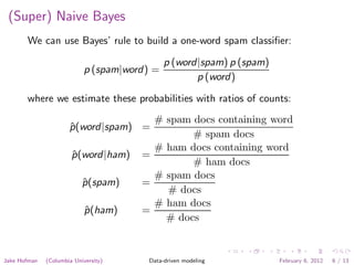
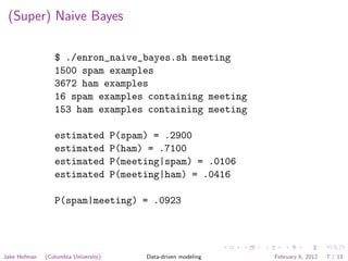
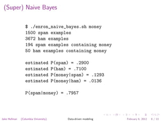
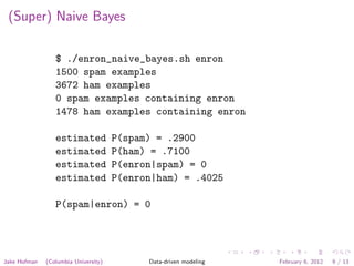
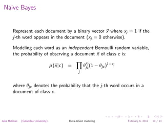
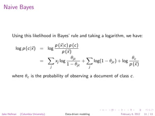
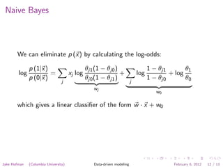
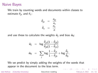
Data-driven modeling
                                           APAM E4990


                                           Jake Hofman

                                          Columbia University


                                         February 6, 2012


Jake Hofman   (Columbia University)        Data-driven modeling   February 6, 2012   1 / 13
Diagnoses a la Bayes1


              • You’re testing for a rare disease:
                  • 1% of the population is infected
              • You have a highly sensitive and specific test:
                  • 99% of sick patients test positive
                  • 99% of healthy patients test negative
              • Given that a patient tests positive, what is probability the
                   patient is sick?


              1
                  Wiggins, SciAm 2006
Jake Hofman       (Columbia University)   Data-driven modeling       February 6, 2012   2 / 13
Diagnoses a la Bayes


                                           Population
                                           10,000 ppl


                              1% Sick                        99% Healthy
                              100 ppl                          9900 ppl

               99% Test +             1% Test -     1% Test +      99% Test -
                 99 ppl                 1 per         99 ppl        9801 ppl


Jake Hofman   (Columbia University)         Data-driven modeling            February 6, 2012   3 / 13
Diagnoses a la Bayes

                                           Population
                                           10,000 ppl


                              1% Sick                        99% Healthy
                              100 ppl                          9900 ppl

               99% Test +             1% Test -     1% Test +      99% Test -
                 99 ppl                 1 per         99 ppl        9801 ppl

          So given that a patient tests positive (198 ppl), there is a 50%
                        chance the patient is sick (99 ppl)!


Jake Hofman   (Columbia University)         Data-driven modeling            February 6, 2012   3 / 13
Diagnoses a la Bayes

                                            Population
                                            10,000 ppl


                               1% Sick                        99% Healthy
                               100 ppl                          9900 ppl

                99% Test +             1% Test -     1% Test +      99% Test -
                  99 ppl                 1 per         99 ppl        9801 ppl
              The small error rate on the large healthy population produces
                                   many false positives.


Jake Hofman    (Columbia University)         Data-driven modeling            February 6, 2012   3 / 13
Inverting conditional probabilities


       Bayes’ Theorem
       Equate the far right- and left-hand sides of product rule

                               p (y |x) p (x) = p (x, y ) = p (x|y ) p (y )

       and divide to get the probability of y given x from the probability
       of x given y :
                                        p (x|y ) p (y )
                             p (y |x) =
                                            p (x)

       where p (x) =                  y ∈ΩY   p (x|y ) p (y ) is the normalization constant.


Jake Hofman   (Columbia University)                Data-driven modeling           February 6, 2012   4 / 13
Diagnoses a la Bayes


       Given that a patient tests positive, what is probability the patient
       is sick?
                                           99/100       1/100

                                        p (+|sick) p (sick)              99   1
                  p (sick|+) =                                      =       =
                                              p (+)                     198   2
                                      99/1002 +99/1002 =198/1002

       where p (+) = p (+|sick) p (sick) + p (+|healthy ) p (healthy ).


Jake Hofman   (Columbia University)          Data-driven modeling                 February 6, 2012   5 / 13
(Super) Naive Bayes
       We can use Bayes’ rule to build a one-word spam classifier:

                                              p (word|spam) p (spam)
                            p (spam|word) =
                                                     p (word)

       where we estimate these probabilities with ratios of counts:
                                         # spam docs containing word
                      p (word|spam) =
                      ˆ
                                                # spam docs
                                         # ham docs containing word
                       p (word|ham)
                       ˆ               =
                                                # ham docs
                                         # spam docs
                           p (spam)
                           ˆ           =
                                           # docs
                                         # ham docs
                            p (ham)
                            ˆ          =
                                           # docs


Jake Hofman   (Columbia University)     Data-driven modeling           February 6, 2012   6 / 13
(Super) Naive Bayes

                 $ ./enron_naive_bayes.sh meeting
                 1500 spam examples
                 3672 ham examples
                 16 spam examples containing meeting
                 153 ham examples containing meeting

                 estimated            P(spam) = .2900
                 estimated            P(ham) = .7100
                 estimated            P(meeting|spam) = .0106
                 estimated            P(meeting|ham) = .0416

                 P(spam|meeting) = .0923


Jake Hofman   (Columbia University)         Data-driven modeling   February 6, 2012   7 / 13
(Super) Naive Bayes

                 $ ./enron_naive_bayes.sh money
                 1500 spam examples
                 3672 ham examples
                 194 spam examples containing money
                 50 ham examples containing money

                 estimated            P(spam) = .2900
                 estimated            P(ham) = .7100
                 estimated            P(money|spam) = .1293
                 estimated            P(money|ham) = .0136

                 P(spam|money) = .7957


Jake Hofman   (Columbia University)         Data-driven modeling   February 6, 2012   8 / 13
(Super) Naive Bayes

                 $ ./enron_naive_bayes.sh enron
                 1500 spam examples
                 3672 ham examples
                 0 spam examples containing enron
                 1478 ham examples containing enron

                 estimated            P(spam) = .2900
                 estimated            P(ham) = .7100
                 estimated            P(enron|spam) = 0
                 estimated            P(enron|ham) = .4025

                 P(spam|enron) = 0


Jake Hofman   (Columbia University)         Data-driven modeling   February 6, 2012   9 / 13
Naive Bayes


       Represent each document by a binary vector x where xj = 1 if the
       j-th word appears in the document (xj = 0 otherwise).

       Modeling each word as an independent Bernoulli random variable,
       the probability of observing a document x of class c is:
                                                          x
                                      p (x|c) =          θjcj (1 − θjc )1−xj
                                                     j


       where θjc denotes the probability that the j-th word occurs in a
       document of class c.


Jake Hofman   (Columbia University)           Data-driven modeling             February 6, 2012   10 / 13
Naive Bayes


       Using this likelihood in Bayes’ rule and taking a logarithm, we have:

                                          p (x|c) p (c)
          log p (c|x) = log
                                              p (x)
                                                   θjc                                       θc
                              =           xj log         +            log(1 − θjc ) + log
                                                 1 − θjc                                    p (x)
                                      j                           j

       where θc is the probability of observing a document of class c.


Jake Hofman   (Columbia University)            Data-driven modeling                  February 6, 2012   11 / 13
Naive Bayes


       We can eliminate p (x) by calculating the log-odds:

              p (1|x)                          θj1 (1 − θj0 )                      1 − θj1       θ1
        log           =               xj log                  +              log           + log
              p (0|x)                          θj0 (1 − θj1 )                      1 − θj0       θ0
                                 j                                       j
                                                  wj
                                                                                      w0

       which gives a linear classifier of the form w · x + w0


Jake Hofman   (Columbia University)               Data-driven modeling                      February 6, 2012   12 / 13
Naive Bayes
       We train by counting words and documents within classes to
       estimate θjc and θc :

                                               ˆ            njc
                                               θjc     =
                                                            nc
                                                  ˆ         nc
                                                  θc   =
                                                            n
       and use these to calculate the weights wj and bias w0 :
                                              ˆ           ˆ

                                                   ˆ        ˆ
                                                   θj1 (1 − θj0 )
                                      ˆ
                                      wj   = log
                                                   ˆ        ˆ
                                                   θj0 (1 − θj1 )
                                                             ˆ
                                                         1 − θj1      ˆ
                                                                      θ1
                                      w0 =
                                      ˆ            log           + log .
                                                             ˆ
                                                         1 − θj0      ˆ
                                                                      θ0
                                              j

       We we predict by simply adding the weights of the words that
       appear in the document to the bias term.
Jake Hofman   (Columbia University)           Data-driven modeling         February 6, 2012   13 / 13
Naive Bayes


              In practice, this works better than one might expect given its
                                        simplicity2


              2
                  http://www.jstor.org/pss/1403452
Jake Hofman       (Columbia University)   Data-driven modeling     February 6, 2012   14 / 13
Naive Bayes


         Training is computationally cheap and scalable, and the model is
                      easy to update given new observations2


              2
                  http://www.springerlink.com/content/wu3g458834583125/
Jake Hofman       (Columbia University)   Data-driven modeling      February 6, 2012   14 / 13
Naive Bayes


                     Performance varies with document representations and
                               corresponding likelihood models2


              2
                  http://ceas.cc/2006/15.pdf
Jake Hofman       (Columbia University)   Data-driven modeling      February 6, 2012   14 / 13
Naive Bayes


              It’s often important to smooth parameter estimates (e.g., by
                         adding pseudocounts) to avoid overfitting


Jake Hofman   (Columbia University)   Data-driven modeling        February 6, 2012   14 / 13

Data-driven Modeling: Lecture 03

  • 1.
    Data-driven modeling APAM E4990 Jake Hofman Columbia University February 6, 2012 Jake Hofman (Columbia University) Data-driven modeling February 6, 2012 1 / 13
  • 2.
    Diagnoses a laBayes1 • You’re testing for a rare disease: • 1% of the population is infected • You have a highly sensitive and specific test: • 99% of sick patients test positive • 99% of healthy patients test negative • Given that a patient tests positive, what is probability the patient is sick? 1 Wiggins, SciAm 2006 Jake Hofman (Columbia University) Data-driven modeling February 6, 2012 2 / 13
  • 3.
    Diagnoses a laBayes Population 10,000 ppl 1% Sick 99% Healthy 100 ppl 9900 ppl 99% Test + 1% Test - 1% Test + 99% Test - 99 ppl 1 per 99 ppl 9801 ppl Jake Hofman (Columbia University) Data-driven modeling February 6, 2012 3 / 13
  • 4.
    Diagnoses a laBayes Population 10,000 ppl 1% Sick 99% Healthy 100 ppl 9900 ppl 99% Test + 1% Test - 1% Test + 99% Test - 99 ppl 1 per 99 ppl 9801 ppl So given that a patient tests positive (198 ppl), there is a 50% chance the patient is sick (99 ppl)! Jake Hofman (Columbia University) Data-driven modeling February 6, 2012 3 / 13
  • 5.
    Diagnoses a laBayes Population 10,000 ppl 1% Sick 99% Healthy 100 ppl 9900 ppl 99% Test + 1% Test - 1% Test + 99% Test - 99 ppl 1 per 99 ppl 9801 ppl The small error rate on the large healthy population produces many false positives. Jake Hofman (Columbia University) Data-driven modeling February 6, 2012 3 / 13
  • 6.
    Inverting conditional probabilities Bayes’ Theorem Equate the far right- and left-hand sides of product rule p (y |x) p (x) = p (x, y ) = p (x|y ) p (y ) and divide to get the probability of y given x from the probability of x given y : p (x|y ) p (y ) p (y |x) = p (x) where p (x) = y ∈ΩY p (x|y ) p (y ) is the normalization constant. Jake Hofman (Columbia University) Data-driven modeling February 6, 2012 4 / 13
  • 7.
    Diagnoses a laBayes Given that a patient tests positive, what is probability the patient is sick? 99/100 1/100 p (+|sick) p (sick) 99 1 p (sick|+) = = = p (+) 198 2 99/1002 +99/1002 =198/1002 where p (+) = p (+|sick) p (sick) + p (+|healthy ) p (healthy ). Jake Hofman (Columbia University) Data-driven modeling February 6, 2012 5 / 13
  • 8.
    (Super) Naive Bayes We can use Bayes’ rule to build a one-word spam classifier: p (word|spam) p (spam) p (spam|word) = p (word) where we estimate these probabilities with ratios of counts: # spam docs containing word p (word|spam) = ˆ # spam docs # ham docs containing word p (word|ham) ˆ = # ham docs # spam docs p (spam) ˆ = # docs # ham docs p (ham) ˆ = # docs Jake Hofman (Columbia University) Data-driven modeling February 6, 2012 6 / 13
  • 9.
    (Super) Naive Bayes $ ./enron_naive_bayes.sh meeting 1500 spam examples 3672 ham examples 16 spam examples containing meeting 153 ham examples containing meeting estimated P(spam) = .2900 estimated P(ham) = .7100 estimated P(meeting|spam) = .0106 estimated P(meeting|ham) = .0416 P(spam|meeting) = .0923 Jake Hofman (Columbia University) Data-driven modeling February 6, 2012 7 / 13
  • 10.
    (Super) Naive Bayes $ ./enron_naive_bayes.sh money 1500 spam examples 3672 ham examples 194 spam examples containing money 50 ham examples containing money estimated P(spam) = .2900 estimated P(ham) = .7100 estimated P(money|spam) = .1293 estimated P(money|ham) = .0136 P(spam|money) = .7957 Jake Hofman (Columbia University) Data-driven modeling February 6, 2012 8 / 13
  • 11.
    (Super) Naive Bayes $ ./enron_naive_bayes.sh enron 1500 spam examples 3672 ham examples 0 spam examples containing enron 1478 ham examples containing enron estimated P(spam) = .2900 estimated P(ham) = .7100 estimated P(enron|spam) = 0 estimated P(enron|ham) = .4025 P(spam|enron) = 0 Jake Hofman (Columbia University) Data-driven modeling February 6, 2012 9 / 13
  • 12.
    Naive Bayes Represent each document by a binary vector x where xj = 1 if the j-th word appears in the document (xj = 0 otherwise). Modeling each word as an independent Bernoulli random variable, the probability of observing a document x of class c is: x p (x|c) = θjcj (1 − θjc )1−xj j where θjc denotes the probability that the j-th word occurs in a document of class c. Jake Hofman (Columbia University) Data-driven modeling February 6, 2012 10 / 13
  • 13.
    Naive Bayes Using this likelihood in Bayes’ rule and taking a logarithm, we have: p (x|c) p (c) log p (c|x) = log p (x) θjc θc = xj log + log(1 − θjc ) + log 1 − θjc p (x) j j where θc is the probability of observing a document of class c. Jake Hofman (Columbia University) Data-driven modeling February 6, 2012 11 / 13
  • 14.
    Naive Bayes We can eliminate p (x) by calculating the log-odds: p (1|x) θj1 (1 − θj0 ) 1 − θj1 θ1 log = xj log + log + log p (0|x) θj0 (1 − θj1 ) 1 − θj0 θ0 j j wj w0 which gives a linear classifier of the form w · x + w0 Jake Hofman (Columbia University) Data-driven modeling February 6, 2012 12 / 13
  • 15.
    Naive Bayes We train by counting words and documents within classes to estimate θjc and θc : ˆ njc θjc = nc ˆ nc θc = n and use these to calculate the weights wj and bias w0 : ˆ ˆ ˆ ˆ θj1 (1 − θj0 ) ˆ wj = log ˆ ˆ θj0 (1 − θj1 ) ˆ 1 − θj1 ˆ θ1 w0 = ˆ log + log . ˆ 1 − θj0 ˆ θ0 j We we predict by simply adding the weights of the words that appear in the document to the bias term. Jake Hofman (Columbia University) Data-driven modeling February 6, 2012 13 / 13
  • 16.
    Naive Bayes In practice, this works better than one might expect given its simplicity2 2 http://www.jstor.org/pss/1403452 Jake Hofman (Columbia University) Data-driven modeling February 6, 2012 14 / 13
  • 17.
    Naive Bayes Training is computationally cheap and scalable, and the model is easy to update given new observations2 2 http://www.springerlink.com/content/wu3g458834583125/ Jake Hofman (Columbia University) Data-driven modeling February 6, 2012 14 / 13
  • 18.
    Naive Bayes Performance varies with document representations and corresponding likelihood models2 2 http://ceas.cc/2006/15.pdf Jake Hofman (Columbia University) Data-driven modeling February 6, 2012 14 / 13
  • 19.
    Naive Bayes It’s often important to smooth parameter estimates (e.g., by adding pseudocounts) to avoid overfitting Jake Hofman (Columbia University) Data-driven modeling February 6, 2012 14 / 13