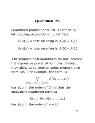
This document summarizes a paper on Boolean programs and quantified propositional proof systems. It introduces quantified propositional proof systems that extend propositional proof systems with propositional quantifiers. The main ideas are that quantified propositional proofs can be witnessed by Boolean programs, and that evaluating these programs is PSPACE-complete if the proofs are not tree-like, showing a connection between quantified propositional proof complexity and computational complexity classes.

1. Boolean Programs and
Quantified Propositional Proof
Systems
To appear in the Bulletin of the Section of Logic
Stephen Cook and Michael Soltys
1

2. A propositional proof is a derivation of a
propositional tautology (e.g. ¬P ∨ P) using a
set of rules.
A nice example of a propositional proof
system is Gentzen’s PK system, where we
have sequents of propositional formulas of
the form:
A1, . . . , An → B1, . . . , Bm (∗)
and the semantics of sequents is given as
follows. We say that a truth assignment τ
satisfies the sequent (∗) iff either τ falsifies
some Ai or τ satisfies some Bi.
For example, if τ is given by P = 0, Q = 1,
R = 0 then τ satisfies
P ∨ Q, ¬R → Q ∧ ¬R
2

3. A sequent is equivalent to the formula
(A1 ∧ · · · ∧ An) ⊃ (B1 ∨ · · · ∨ Bm)
In other words, the conjunction of the Ai’s
implies the disjunction of the Bi’s.
We say that a sequent is valid if it is true
under all truth assignments. For example, the
following are valid sequents:
A → A
→ A, ¬A
A, ¬A →
→ A ∨ ¬A
A, A ⊃ B → B
A PK proof is a sequence of sequents, where
all the sequents are derived from previous
sequents or are logical axioms of the form
A → A, → 1 or 0 →.
3

4. PK Rules of inference:
weak
Γ → ∆
A, Γ → ∆
Γ → ∆
Γ → ∆, A
exch
Γ1, A, B, Γ2 → ∆
Γ1, B, A, Γ2 → ∆
Γ → ∆1, A, B, ∆2
Γ → ∆1, B, A, ∆2
cont
Γ, A, A → ∆
Γ, A → ∆
Γ → ∆, A, A
Γ → ∆, A
“¬”
Γ → ∆, A
¬A, Γ → ∆
A, Γ → ∆
Γ → ∆, ¬A
“∧”
A, B, Γ → ∆
(A ∧ B), Γ → ∆
Γ → ∆, A Γ → ∆, B
Γ → ∆, (A ∧ B)
“∨”
A, Γ → ∆ B, Γ → ∆
(A ∨ B), Γ → ∆
Γ → ∆, A, B
Γ → ∆, (A ∨ B)
cut
Γ → ∆, A A, Γ → ∆
Γ → ∆
4

5. Any valid sequent can be derived from initial
sequents of the form A → A, → 1 and 0 →,
using the above rules (completeness of PK),
and only valid sequents can be derived
(soundness of PK).
As an example we give a proof of one of
DeMorgan’s laws:
¬(P ∧ Q) → ¬P ∨ ¬Q
Here is the derivation:
P → P
→ P, ¬P
→ P, ¬P, ¬Q
Q → Q
Q → Q, ¬P
→ Q, ¬P, ¬Q
→ P ∧ Q, ¬P, ¬Q
→ P ∧ Q, ¬P ∨ ¬Q
¬(P ∧ Q) → ¬P ∨ ¬Q
5

6. Abstract Definition: A proof system is a
feasible (i.e. easily computable) map
f : {0, 1}∗ onto
−→ {tautologies}
Where {tautologies} is just the set of
propositional tautologies, and if f(x) = A
then x is the proof of the propositional
tautology A.
A proof system is polynomially bounded if
there exists a polynomial p such that for
every A ∈ {tautologies}, there exists an x
such that |x| ≤ p(|A|), i.e. every tautology has
a proof which is “proportional” to its size.
See “The Complexity of Propositional
Proofs”, by Alasdair Urquhart, in The
Bulletin of Symbolic Logic, December 1995,
for all the details.
6

7. Interest in propositional proof complexity
arose from two fields connected with
computers: automated theorem proving
(artificial intelligence) and computational
complexity theory.
Some Complexity Theory
P is the class of problems that can be solved
with algorithms that run in polynomial time
in the size of the input (e.g. given a truth
assignment τ, and a sequent S, does τ satisfy
S?).
NP is the class of problems whose solutions
can be verified by an algorithm that runs in
polynomial time (e.g. given a sequent S, is it
satisfiable?)
co-NP is the class of problems for which a
counter-example can be verified by an
algorithm that runs in polynomial time (e.g.
given a sequent S, is it valid?).
7

8. Theorem: NP = co-NP iff there is a
polynomially bounded proof system for the
propositional tautologies.
Also P = NP implies NP = co-NP, thus if we
prove that there is no polynomially bounded
proof system (which is what experts
conjecture), then it will follow that
NP = co-NP, and therefore P = NP.
The problem
P
?
= NP
has been listed by Steve Smale in the top
three “Mathematical Problems for the Next
Century” (Math Intelligencer 20, 1998).
8

9. How could we prove that there is no
polynomially bounded proof system? It seems
like a very difficult problem. The standard
approach is to consider stronger and stronger
proof systems, and to exhibit superpolynomial
lower bounds for each of them.
strongest Quantified PK
Extended PK
PK
————————
Bounded Depth PK
Resolution
weakest Truth Tables
However, we can only prove superpolynomial
lower bounds for the weaker systems (the
ones below the line). The systems above the
line have no known lower bounds.
9

10. Quantified PK
Quantified propositional PK is formed by
introducing propositional quantifiers:
∀xA(x) whose meaning is A(0) ∧ A(1)
∃xA(x) whose meaning is A(0) ∨ A(1)
The propositional quantifiers do not increase
the expressive power of formulas. Instead,
they allow us to shorten some propositional
formulas. For example, the formula
(x1,...,xn)∈{0,1}n
A(x1, . . . , xn)
has size in the order of 2n|A|, but the
equivalent quantified formula
∃x1 . . . ∃xnA(x1, . . . , xn)
has size in the order of n + |A|.
10

11. The quantified propositional calculus is first
discussed by B. Russell in “The Theory of
Implication”, American Journal of
Mathematics in 1906. Also, the Polish
mathematician Le´sniewski treated it in his
“Protothetic”.
Martin Dowd investigated the connection
between quantified propositional proof
systems and the complexity class PSPACE in
his PhD thesis in 1979.
A modest source of information is also a 5
page section in Jan Kraj´ıˇcek’s book
“Bounded Arithmetic, Propositional Logic,
and Complexity Theory”, 1995.
Still, little is known about quantified
propositional proof systems.
11

12. G is PK with ∃ and ∀
I follow the results and notation from Jan
Kraj´ıˇcek’s “Bounded Arithmetic,
Propositional Logic, and Complexity Theory”.
The quantified propositional proof system G
extends LK by allowing quantified
propositional formulas in sequents, and by
adding the following quantifier rules:
A(B), Γ → ∆
∀xA(x), Γ → ∆
Γ → ∆, A(p)
Γ → ∆, ∀xA(x)
A(p), Γ → ∆
∃xA(x), Γ → ∆
Γ → ∆, A(B)
Γ → ∆, ∃xA(x)
where B is any formula, and with the
restriction that the atom p does not occur in
the lower sequents of ∀-right and ∃-left.
12

13. Let G1 be the restriction of G where we allow
only strict Σ
q
1 formulas, that is, all formulas
must begin with a block of existential
quantifiers (possibly empty) followed by a
quantifier free formula. In other words, all
formulas are either quantifier free, or of the
form
∃x1 . . . ∃xnA(x1, . . . , xn)
where A(x1, . . . , xn) is quantifier free.
For example, the sequent
∃x∃y((¬x ∨ p) ∧ (¬y ∨ q)) → ∃x(x ∨ ¬p ∨ q), p ∧ q
has only Σ
q
1 formulas.
13

14. Witnessing
Given a sequent S, we want to have a way of
computing the values of the existential
variables on the right in terms of the free
variables, and the quantified variables on the
left. For example, consider the sequent
∃yA(x, y) → ∃yA(x, y) (∗)
where x, y are the only variables in this
sequent. In this case it is very easy. The
quantified variable y on the right can be
witnessed by the following function:
f(x, y) = y
that is, the sequent
A(x, y) → A(x, f(x, y))
is valid if (∗) was valid.
14

15. Suppose that π is a G1 proof. We show that
the existential quantifiers can be witnessed by
Boolean programs. We do this by induction
on the number of sequents in π.
For example, consider the contraction rule:
C(¯p) → D(¯p), ∃xB(x), ∃xB(x)
C(¯p) → D(¯p), ∃xB(x)
By Induction Hypothesis, we know that there
are Boolean programs g, h such that the
sequent
C(¯p) → D(¯p), B(g(¯p)), B(h(¯p))
is valid. Now, define f as follows:
f(¯p) =



g(¯p) if B(g(¯p))
h(¯p) otherwise
The bottom sequent can thus be converted
to the valid sequent
C(¯p) → D(¯p), B(f(¯p)),
15

16. Main Idea
If π is a G1 proof of a propositional tautology,
and π is tree-like, then the existential
quantifiers can be feasibly computed by
evaluating Boolean circuits. This was already
shown in Jan Kraj´ıˇcek’s book “Bounded
Arithmetic, Propositional Logic, and
Complexity Theory”.
If, on the other hand, π is not tree-like, then
it seems that evaluating the existential
quantifiers requires a lot of computational
power, i.e. Boolean programs whose
evaluation is a PSPACE complete problem.
This is shown in our paper “Boolean
Programs and Quantified Propositional Proof
Systems”.
16

17. References
“Boolean Programs and Quantified
Propositional Proof Systems”, by S.Cook and
M. Soltys, in this paper we introduce the
notion of Boolean programs, and we
characterize PSPACE in terms of families of
Boolean programs. We then show how to use
Boolean programs to witness quantifiers in
G1.
“The Complexity of Propositional Proofs”, by
Alasdair Urquhart, in The Bulletin of
Symbolic Logic, December 1995, a
comprehensive introduction to the complexity
of propositional proofs.
“Bounded Arithmetic, Propositional Logic,
and Complexity Theory”, by Jan Kraj´ıˇcek. A
short introduction to quantified propositional
proof systems.
17