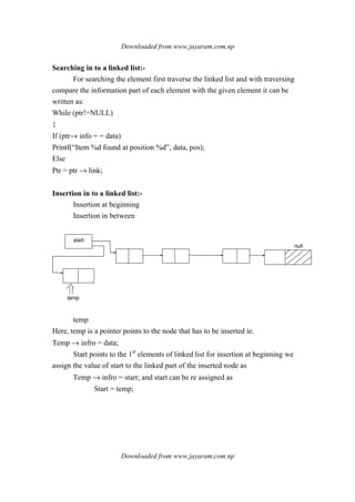
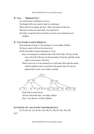
1. Linear data structures like arrays, stacks, queues, and linked lists process data items in a linear fashion.
2. Stacks follow a last-in, first-out principle where the last item inserted is the first removed.
3. Queues follow a first-in, first-out principle where the first item inserted is the first removed.
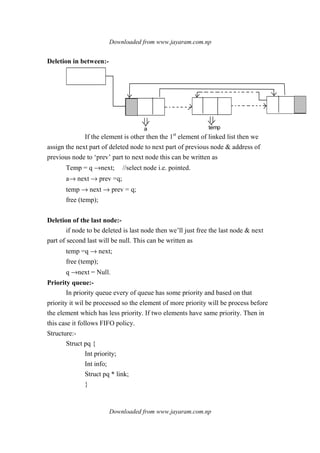
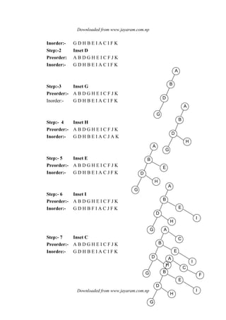
![- Deletion
- Search
- Display
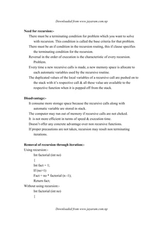
Here, item is component of ADT.
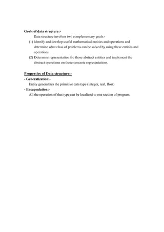
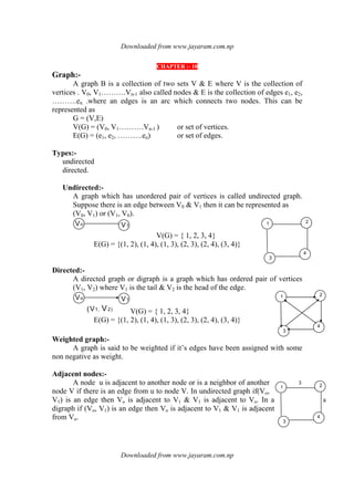
An ADT consists of two parts.
(a) value definition
i. Definition clause
ii. Condition clause
(b) operator definition
# ADT for Relation:-
/*value of definition */
Abstract type def <integer, integer> RTIONAL // value definition
Condition RATIONAL [1] = 0; // denominator is not equal to zero;
condn
.
/* operator definition * /
Abstract RATIONAL make rational (a, b)
Int a,b;
Precondition b! = 0;
Post condition make rational [0] == a;
Make rational [1] == b;
Abstract RATIONAL add (a, b)
RATIONAL a,b;
Past condition add [1] == a[1] * b[1];
Add [0] == a[a] * b[1] + b[0] * a[1];
Abstract RATIONAL mult (a,b)
RATIOANL a, b;
Post condition mult [0] ==a[a] * b[0];
Mult [1] == a[1] *b[1];
Abstract RATIONAL equal (a,b)
RATIONAL a,b;
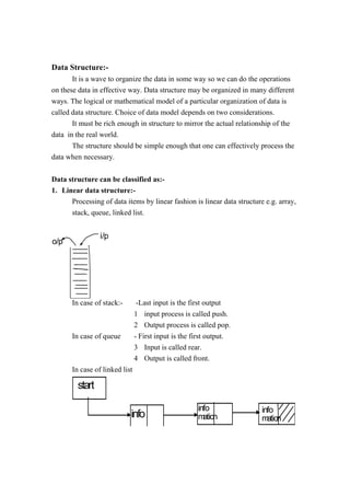
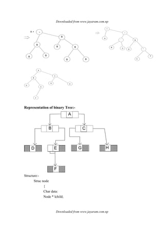
Post condition equal == (a[0] * b[1] == b [0] * a[1]);](https://image.slidesharecdn.com/datastructureandalgorithm-141219101030-conversion-gate01/85/Data-structure-and-algorithm-dsa-3-320.jpg)
![Downloaded from www.jayaram.com.np
Downloaded from www.jayaram.com.np
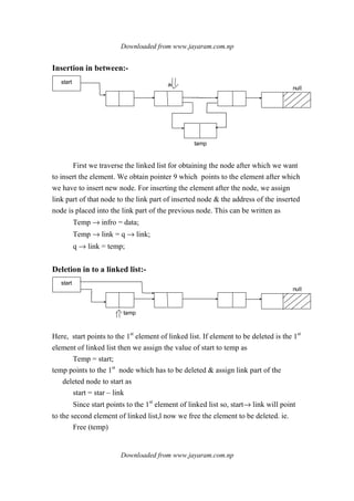
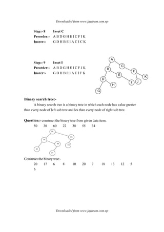
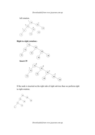
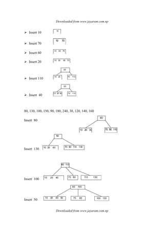
Stack Implementation:-
(i) Array implementation
(ii) Linked list.
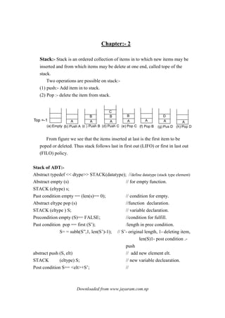
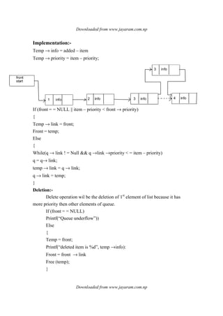
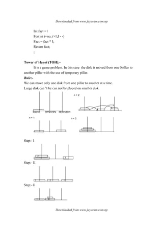
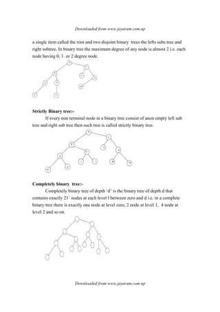
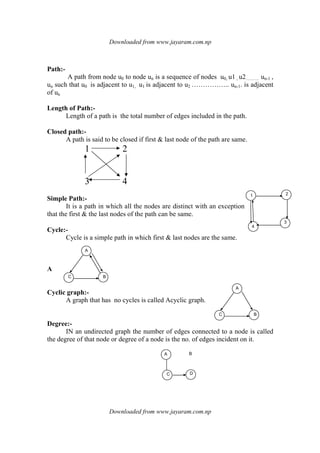
Array Implementation:-
In Array we can push elements one by one from 0th
position 1st
position
…….. n-1th
position. Any element can be added or deleted at any place and we can
push or pop the element from the top of the stack only.
1. When there is no place for adding the element in the array, then this is
called stack overflow. So first we check the value of top with size of array.
2. When there is no element in stack, then value of top will be -1. so we check
the value of top before deleting the element of stack.
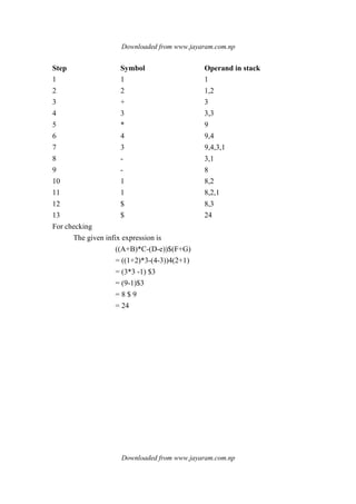
5 10 15
Stack_array [0] [1] [2] [3] [4] [5] [6]
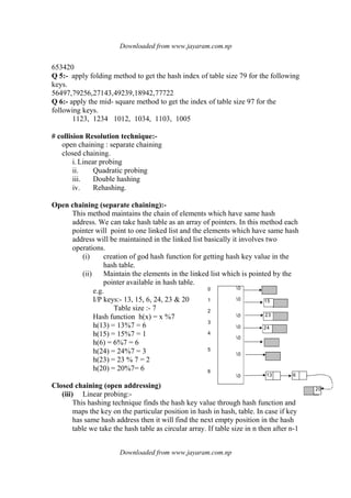
Here, Stack is implemented with stack array, size of stack array is 7 and value
of top is 2.
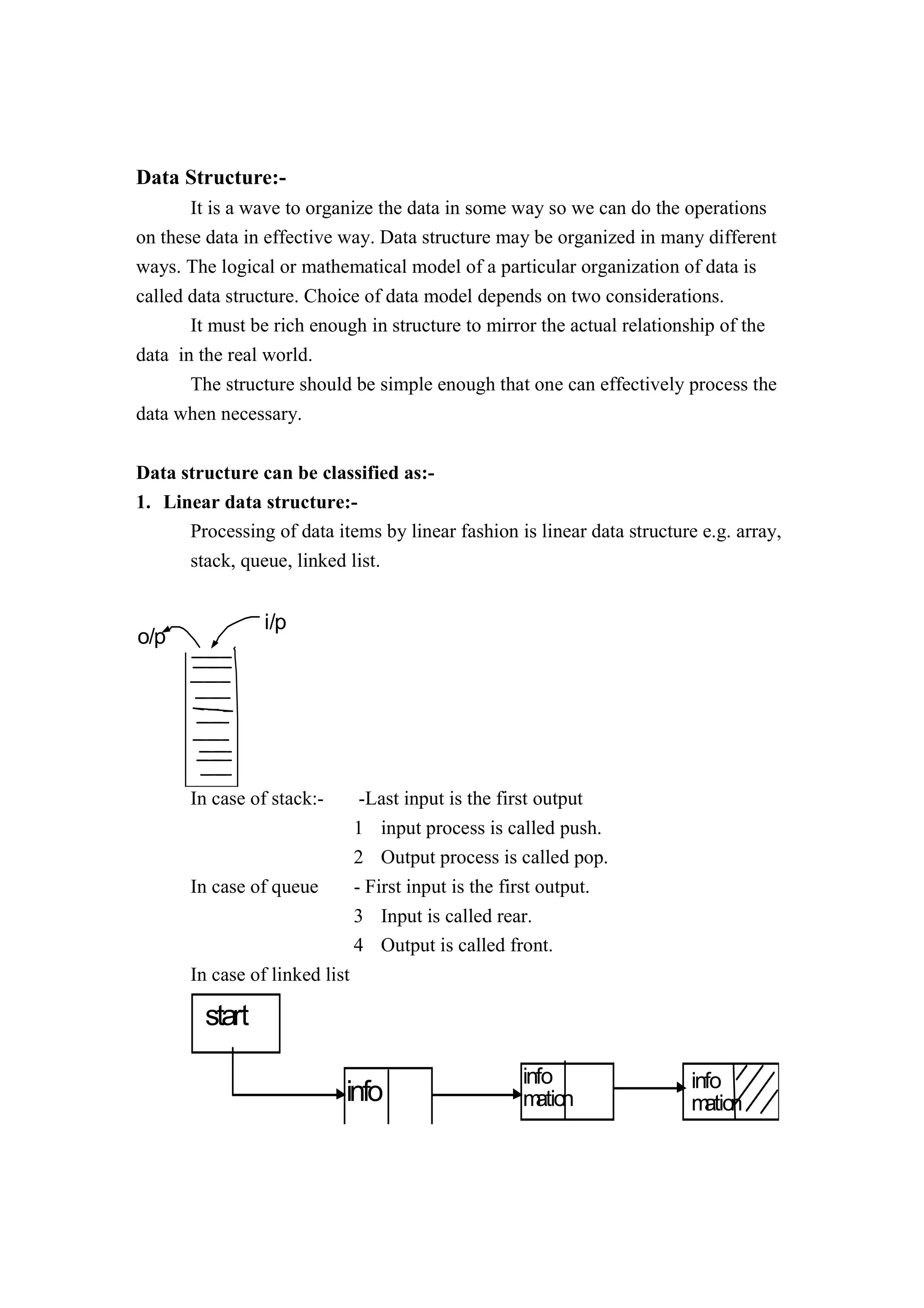
Operation of Stack:-
Push Operation:-
If (top == (max-1)]
Printf(“stack over flow”);
Else
{
Top == top + 1;
Stack_arr[top] = pushed –item;
}
Pop Operation:-
If (top ==-1)
Printf(“stack underflow”);
Else
{
Printf(“Poped element is %d”,stack_arr[top]);](https://image.slidesharecdn.com/datastructureandalgorithm-141219101030-conversion-gate01/85/Data-structure-and-algorithm-dsa-6-320.jpg)
![Downloaded from www.jayaram.com.np
Downloaded from www.jayaram.com.np
Top= top – 1;
}
Algorithm for push & Pop
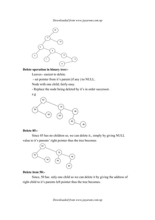
PUSH:-
Let stack [Max size] is an array for implementing the stack
1. [check for stack overflow?]
If top = maxsize-1, then print overflow & exit
2. set top = top + 1 (increase top by 1)
3. set stack [top] = item (inserts item in new top position )
4. exit.
POP:-
1. check for the stack underflow
If Top <0 then
Print stack underflow and exit
Else
[Remove the top element]
Set item = stack [ top]
2. Decrement the stack top.
3. Return the deleted item from the stack.
4. Exit.
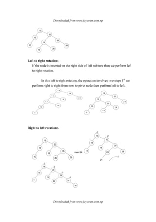
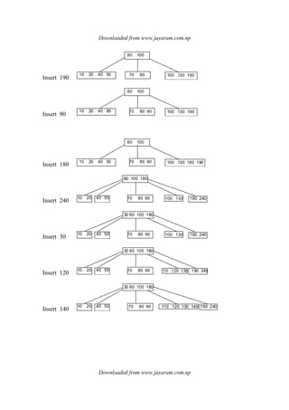
Application of Stack:-
1 Conversion of an expression from infix to post fix.
2 Evaluation of an arithmetic expression from post fix expression.
Precedence:-
$ (Power), %( remainder) - 5
*(mul), /(div) - 4
+ (add), -(sub) - 3
( -2
) - 1](https://image.slidesharecdn.com/datastructureandalgorithm-141219101030-conversion-gate01/85/Data-structure-and-algorithm-dsa-7-320.jpg)
![Downloaded from www.jayaram.com.np
Downloaded from www.jayaram.com.np
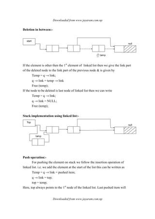
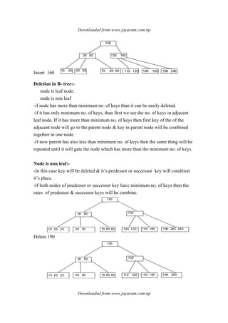
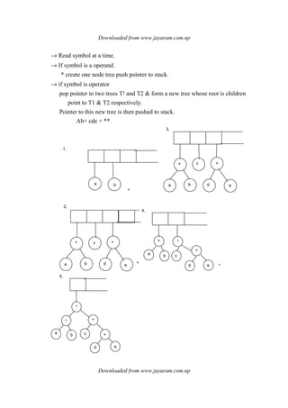
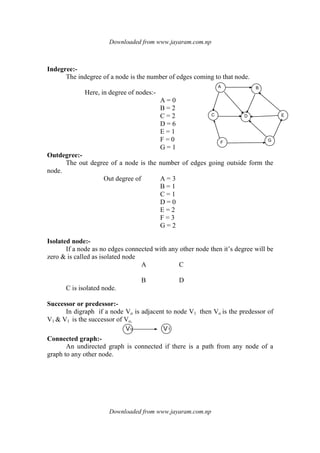
Algorithm:-
(i) Add the unique symbol # at the end of array post fix.
(ii) Scan the symbol of array post fix one by one from left to right.
(iii) If symbol is operand, two push in to stack.
(iv) If symbol is operator, then pop last two element of stack and evaluate it as
[top- 1] operator [top] & push it to stack.
(v) Do the same process until ‘#’ comes in scanning.
(vi) Pop the element of stack which will be value of evaluation of post fix
arithmetic expression.
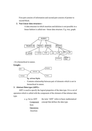
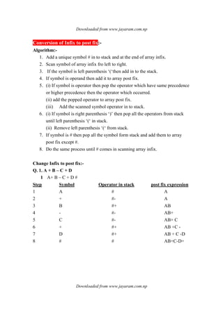
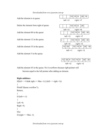
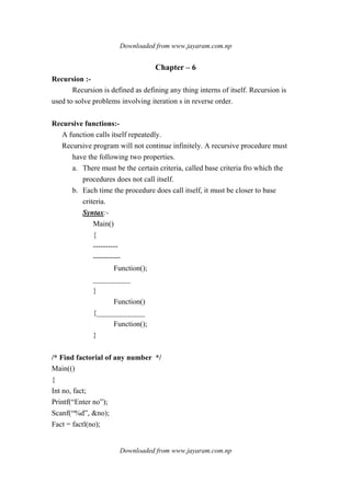
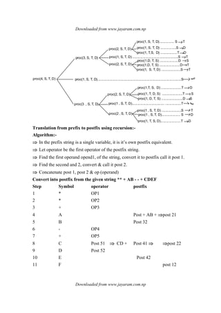
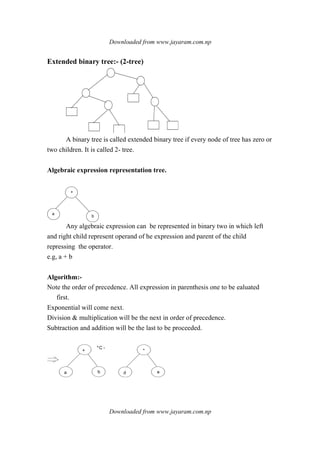
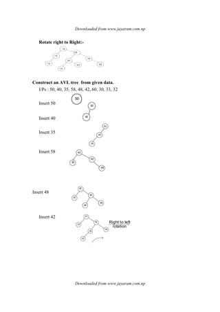
Postfix expression ABCD $+* EF$GHI * -
Evaluate postfix expression where A = 5, B = 5, C = 4, D = 2 E = 2, F= 2 ,
G = 9, H= 3 now, 4, 5, 2, $ , +, *, 2, 2, $, 9, 3, /, *, - , #
Step Symbol Operand in stack
1 4 4
2 5 4, 5
3 4 4,5,4
4 2 4,5,4,2
5 $ 4,5,16
6 + 4,21
7 * 84
8 2 84,2
9 2 84, 2,2
10 $ 84,4
11 9 84,4,9
12 3 84,4,9,3
13 / 84, 4, 3
14 * 84,12
15 - 72
The required value of postfix expression is 72](https://image.slidesharecdn.com/datastructureandalgorithm-141219101030-conversion-gate01/85/Data-structure-and-algorithm-dsa-10-320.jpg)
![Downloaded from www.jayaram.com.np
Downloaded from www.jayaram.com.np
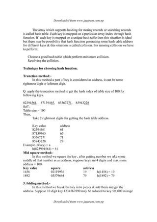
Chapter:- 3
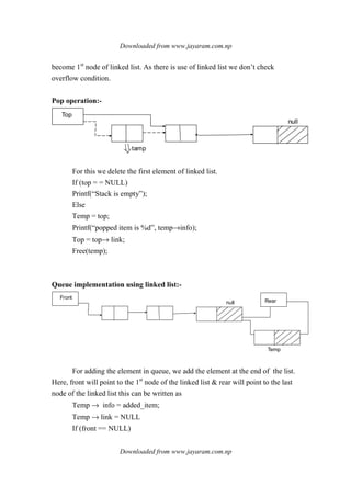
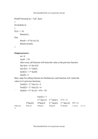
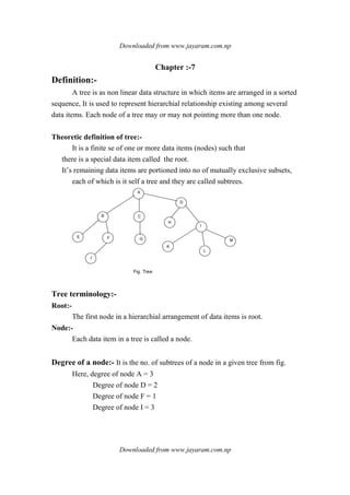
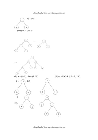
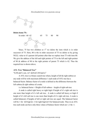
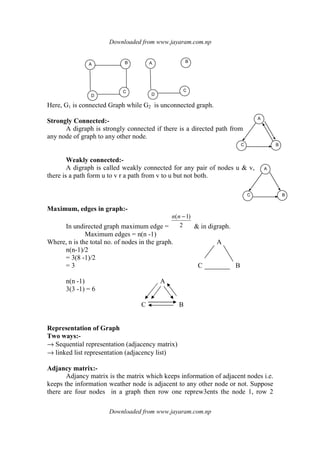
Queue:-
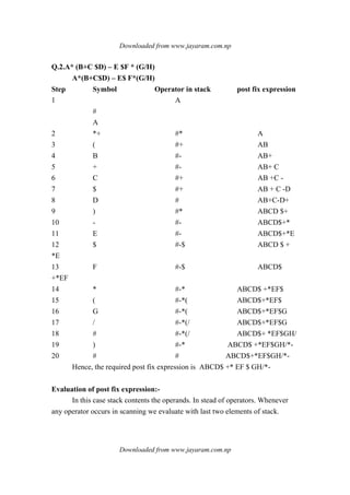
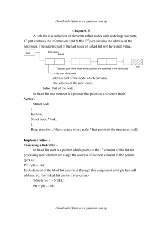
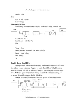
A queue is an ordered collections of items from which items may be
deleted at one end called the front of the queue and in to which items may be
inserted at the other end called rear of the queue.
Deletion ⇒ ⇐ Insertion
Front rear
e.g.
queue – arr [5] [0] [1] [2] [3] [4]
front =-1 (a) empty queue.
Rear =-1
5
Front =0 fig:- adding an item in queue
Rear =0
5 1 0
Front =0 fig:- adding an item in queue
Rear = 1
5 1 0 15
Front =0
Rear =2 fig:- adding an item in queue.
1 0 15
Front = 1 fig:- deleting an element from queue
Rear =2
1 0 15 20
Front = 1
Rear = 3 fig:- adding an element in queue
from figure we see that item are inserted at rear end and deleted at front
end. Thus queue follows FIFO policy. (First in first out).](https://image.slidesharecdn.com/datastructureandalgorithm-141219101030-conversion-gate01/85/Data-structure-and-algorithm-dsa-13-320.jpg)
![Downloaded from www.jayaram.com.np
Downloaded from www.jayaram.com.np
Queue as an A-DT
Abstract typedef <<eltype>>QUEUE (eltype); //queue type element.
Abstract empty (q)
QUEUE (eltype) q;
Post condition empty = = (len (q) = =0);
Abstract eltype delete (q)
QUEUE(eltype ) q;
Pre condition empty (q) = = FALSE
Post condition remove = = front (q’);
q = = sub(q’, 1, len(q’-1);
abstract insert (q, elt)
QUEUE (eltype) q;
Eltype elt ;
Post condition insert = rear (q’);
Q = q’+<elt>;
Queue Implementation :-
8 array implementation
9 linked list implementation
Array implementation of Queue:-
A queue top two pointers front and rear pointing to the front and rear
element of the queue.
- when there is no place for adding elements in queue, then this is called queue
overflow.
- when there is no element for deleting from queue, then value of front and rarer
will be -1 or front will be greater then rarer.
[0] [1] [2] [3] [4]
5 10
Front t =1
Rear =1](https://image.slidesharecdn.com/datastructureandalgorithm-141219101030-conversion-gate01/85/Data-structure-and-algorithm-dsa-14-320.jpg)
![Downloaded from www.jayaram.com.np
Downloaded from www.jayaram.com.np
Operation in queue
1. Add operation :-
If (rear = = Max -1)
Printf(“queue overflow”);
Else
{
If (front = = -1)
Front = 0;
Rear = rear + 1;
Queue_arr[rear]= added-item;
}
Delete operation:-
If (front = = -1)|| (front >rear)
{
Printf(“Queue under flow”);
Return;
}
Else
Printf(“Element detected from queue”, queue_arr[fornt]);
Front = front +1;
}
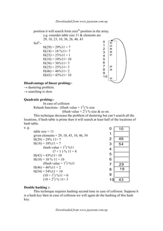
Drawbacks:-
[0] [1] [2] [3] [4]
5 10 1 5
Front =2
Rear = 4
Here we see that the rear is at the last position of array and front is not at
the zeroth
position. But we can not add any element in the queue because the rear
is at the n-1 position.
There are two spaces for adding the elements in queue. But we can not add](https://image.slidesharecdn.com/datastructureandalgorithm-141219101030-conversion-gate01/85/Data-structure-and-algorithm-dsa-15-320.jpg)
![Downloaded from www.jayaram.com.np
Downloaded from www.jayaram.com.np
any element in queue because are is at the last position of array. One way is to
shift all the elements of array to left and change the position of front and rear but it
is not practically good approach. To overcome this type of problem we use the
concept of circular queue.
Algorithm to insert an element in a queue Deletion
Step:-1 Step:-1
[check overflow condition] [check underflow
condition]
If rear (=) > [Max -1] if front =-1
o/p :”over flow” o/p:”under flow & return;
return;
Step:-2 Step:-2
[increment rear pointer] Remove an element
Rear = rear +1 value: Q[Front]
Step:-3 Step:-3
[insert an element ] [check for empty queue]
Q[rear]= value if front = = rear
Front =-1
Step:-4 Rear = -1
[set front pointer] else
If front =-1 front = front +1
Step:-5 Step:-4
Return Return [value]
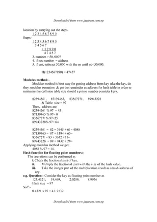
Circular Queue:-
[0] [1] [2] [3] [4]
1 0 20 3 0
A circular queue is one in which the insertion of new element is done at the very
first location of the queue if the last location of the queue is full.
e.g consider C queue_arr[4]](https://image.slidesharecdn.com/datastructureandalgorithm-141219101030-conversion-gate01/85/Data-structure-and-algorithm-dsa-16-320.jpg)
![Downloaded from www.jayaram.com.np
Downloaded from www.jayaram.com.np
a. [0] [1] [2] [3]
5 10 1 5
from = 1 rear = 3.
initial queue
b.
10 1 5
front = 2
fig. deletion in queue rear = 3
c.
10 1 53 5
front =0 rear = 1
fig. addition in queue.
d
10 1 52 035
rear =1
front =2
fig. addition in queue.
e
1 52 035
front =1
rear = 3
fig. deletion in queue.
f
2 035
front = 1
rear =1
fig. deletion in queue
g
2 0
front = 1
rear =1
fig. deletion in queue
h rear = 1
Front =-1
fig. deletion in queue](https://image.slidesharecdn.com/datastructureandalgorithm-141219101030-conversion-gate01/85/Data-structure-and-algorithm-dsa-17-320.jpg)
![Downloaded from www.jayaram.com.np
Downloaded from www.jayaram.com.np
Insersation:-
If ((front == 0 && rear = Max -1 ) || (front = = rear +1))
{
Printf(“Queue overflow”);
Return;
}
If (front = = - 1)
{
Front =0;
Rear = 0;
}
Else
If(rear == Max -1)
Rear =0;
Else
Rear = rear +1;
(queue_arr[rear] = added_item;
Operation
Deletion:-
If (front = = -1
{ printf(“queue underflow”);
Return;
}
Else
Printf(“element deleted from queue is %d”);
(queue_arr[front];
If (front == rear)
{
Front =-1;
Rear = -1;
}
Else](https://image.slidesharecdn.com/datastructureandalgorithm-141219101030-conversion-gate01/85/Data-structure-and-algorithm-dsa-18-320.jpg)
![Downloaded from www.jayaram.com.np
Downloaded from www.jayaram.com.np
5 10 15 8
left =2 right =5
10 15 8
left =3 right =5
10 15 8 20
left =3 right =6
If (front = = Max – 1)
Front = 0;
Else
Front = front +1;
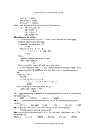
Dequeue (Double ended queue)
In dequeue we can add or delete the element from both sides i.e. front end
or form the rear end. It is of two types.
(i) I/P restricted
(ii) O/P
In input restricted dequeue element can be added at only one end but we
can delete the element from both sides.
In output restricted dequeue eleme4tn can be added from both side but
deletion is allowed only at one end.
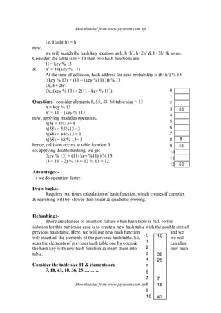
Operation in Dequeue:-
We assume a circular array fro operation of addition or deletion.
[0] [1] [2] [3] [4] [5] [6] [7]
5 10 15
Left = 2
Right = 4
We maintain two pointers right & left which indicate positions of dequeue. Here,
left pointer is at position 2 and right pointer is at position 4.
For I/P restricted:-
Add 8 in the queue from right.
Delete the element from left of the queue
Add the element 20 in the queue](https://image.slidesharecdn.com/datastructureandalgorithm-141219101030-conversion-gate01/85/Data-structure-and-algorithm-dsa-19-320.jpg)
![Downloaded from www.jayaram.com.np
Downloaded from www.jayaram.com.np
Right = 0;
Else
Right = right +1;
Dedequeue_arr[right] = added_item;
Left Addition:-
If (( left == 0 && right == Max-1) || (left == right +1))
{
Printf(“Queue overflow”);
Return;
}
If (left==-1)
{
Left =0;
Right =0;
}
Else
If (left == 0)
Left = Max -1;
Else
Left = left -1;
Dequeue_arr[left] = added_item;
Delete left:-
If (left==-1)
{
Printf(“Queue flow”);
Return;
}
Printf(“Element deletd from queue is “%d”, dequeue_arr[left]. // point delete
item
If (left == right ) // make empty
{
Left ==-1;](https://image.slidesharecdn.com/datastructureandalgorithm-141219101030-conversion-gate01/85/Data-structure-and-algorithm-dsa-21-320.jpg)
![Downloaded from www.jayaram.com.np
Downloaded from www.jayaram.com.np
Right =-1;
}
Else
If(left== Max -1) //move from zero.
Left =0;
Else
Left = left +1; // increase space.
Delete Right:-
If (left ==-1)
{
Printf(“Quieue underflow”);
Return;
}
Printf(“element delected from queue is %d”, deque_arr[right]);
If(left==right)
{
Left =-1;
Right =-1;
}
Else
If(right==0)
Right =Max-1;
Else
Right = right [-1;
}](https://image.slidesharecdn.com/datastructureandalgorithm-141219101030-conversion-gate01/85/Data-structure-and-algorithm-dsa-22-320.jpg)
![Downloaded from www.jayaram.com.np
Downloaded from www.jayaram.com.np
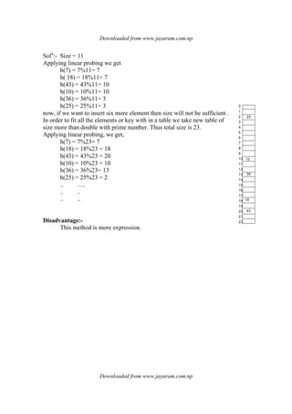
Chapter:- 4
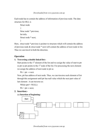
A linear list is an ordered set consisting of a umber of elements to which
addition w& deletion can be made. A linear list displays the relationship of
physical adjenci. The first element of a list is called the hear of list & the last is
called the tail of the list. The next element of the head of the list is called it’s
successes. The previous element to the tail (if it is not head of the list) is called it’s
predessor. Clearly a head doesn’t have as predessor & a tail doesn’t have a
successor. Any other element of the list has both one successor & one predessor.
10 20 30 40 50
head
Operations perform in list:-
1. Traversing an array list
2. Searching an element in the list
3. Insertion of an element in the list
4. Deletion of an element in the list.
Array Implementation:-
Take an array of size 10 which has 5 elements
10 20 30 40 50
[0] [1] [2] [3] [4] [5] [6] [7] [8] [9]
⇒ Traversing an array list:-
Here each element can be found through indeed no. of array & is
incremented by 1.
When index =0.
Then,
Arr[10] = 10 ⇒ determines 1st
element in array
Index = index +1
Then
Arr[index]= 20](https://image.slidesharecdn.com/datastructureandalgorithm-141219101030-conversion-gate01/85/Data-structure-and-algorithm-dsa-23-320.jpg)
![Downloaded from www.jayaram.com.np
Downloaded from www.jayaram.com.np
In this way we can transverse each element of array by incrementing
the index by 1 until index is not greater than no. of elements.
⇒⇒⇒⇒ Searching in an array list:-
For searching an element, we first travers the array list and while traversing
, we compare each element of array with the given element.
Int I, item;
For (i=0;i<n;i++)
‘{
If(item== arr[i])
Return(i+1);
}
Insertion of an element in the list:-
-two ways:-
(i) insertion at end
(ii) insertion in between.
(i) Insertion at end
10 20 30 40 50
60 elemetn inserted at 6th position
Set the array index to the total no of elements & then insert the element
Index = Total no of element (i.e 5)
Arr[index] = value of inserted element
2. Insertion in between
60 elemetn inserted at 4th position
10 20 30 40 50
Shift right one position all array elements from last array element to the
array element before which we want to insert the element.
Int tem, item, position;
If (n = = max)
{](https://image.slidesharecdn.com/datastructureandalgorithm-141219101030-conversion-gate01/85/Data-structure-and-algorithm-dsa-24-320.jpg)
![Downloaded from www.jayaram.com.np
Downloaded from www.jayaram.com.np
Printf(“list overflow”);
Return;
}
If (position >n+1)
{
Printf(“enter position less than or equal to %d”n+1);
Return;
}
If(position = = n+1) /*insertion at the end */
{
Arr [n]= item;
N= n+1;
Return;
}
Temp = n-1 //insertion in between
While (temp>=positon-1)
{
Arr[temp+1] = arr [temp];
Temp - -
}
Arr [positon -1] = item;
n = n+1;
Deletion of an element in the list:-
deletion of the last element
deletion in between
Deletion of the last element:-
10 20 30 40 50
Deleted element
Traverse the array last and if the item is last item of the array, then delete
that element & decrease the total no of element by 1,](https://image.slidesharecdn.com/datastructureandalgorithm-141219101030-conversion-gate01/85/Data-structure-and-algorithm-dsa-25-320.jpg)
![Downloaded from www.jayaram.com.np
Downloaded from www.jayaram.com.np
Deletion in between:-
10 20 30 40 50
Deleted element
First traverse the array list & compare array element with the element
which is to be deleted, then shift left one position from the next element to
the last element of array and decrease the total no. of elements by 1.
Int temp, position , item, n;
If (n= = 0) // present or not element
{
Printf(“list underflow”);
Return;
}
If (item == arr [n-1] //deletion at the end.
{
n = n- 1;
return;
}
Temp = position -1;
While (temp < = n -1)
{
Arr [temp] = arr [temp +1]
Temp + + ;
}
n = n -1;
Advantage of list:-
⇒⇒⇒⇒ Easy to compute the address of the array through index 4 can be access the
array element through index.
Disadvantage:-
⇒⇒⇒⇒ Use of contiguous list which is time consuming.
⇒⇒⇒⇒ As array size is declared we can’t take elements more then array size.
⇒⇒⇒⇒ If the elements are less than the size of array, then there is wastage of memory.](https://image.slidesharecdn.com/datastructureandalgorithm-141219101030-conversion-gate01/85/Data-structure-and-algorithm-dsa-26-320.jpg)
![Downloaded from www.jayaram.com.np
Downloaded from www.jayaram.com.np
⇒⇒⇒⇒ Too many shift operation on each insertion and deletion.
To overcome this problem we use liked list or DLL.
Index to prefix conversion :-
Rules:-
1. Parenthesize the expression starting from left to right.
2. During parenthesizing the expression, the operands associated with
operator having higher precedence are first parenthesized.
e.g. B * C is first parenthesized before A+B in A+B *C
3. the sub expression which has been converted in to prefix is to be treated as
single operand.
4. once the expression is converted to postfix from remove the parenthesis.
Question:- (A*B + (C/D) –F
(A*B + (C/D) –F
((A*B + (C/D)) – F)
((A*B+W) – F) [ W = /CD let]
(( *AB + W) –F)
((X +W)-F [ X = *AB]
(+XW – F)
(Y –F) [ Y = +XW
-YF
-+XWF
- + ABWF
- + * AB/CDF.
Which is required prefix expression.
Dynamic memory allocation:-
In an array it is necessary to declare the size of array. This creates two
possible problems.
If the records that are stored is less than the size of array, then there is a
wastage of memory.](https://image.slidesharecdn.com/datastructureandalgorithm-141219101030-conversion-gate01/85/Data-structure-and-algorithm-dsa-27-320.jpg)
![Downloaded from www.jayaram.com.np
Downloaded from www.jayaram.com.np
If we want to store more records then size of array, we can’t store.
To overcome these problem we use dynamic memory allocation. The
functions used for dynamic memory The functions used for dynamic memory
allocation and deallocaton are :-
Malloc()
Calloc()
Free()
Realloc()
Malloc():-
This function is used to allocate memory space. The malloc () function
reserves a memory space of specified size and gives the strating address to the
pointer variable.
Syntax:-
Ptr = (data type * ) malloc (specified size)
Type of pointer size required to reserve in memory.
Example:-
Ptr = (int *) malloc (10);
Struct student
{
Int roll_no;
Char name [30];
Float percentage;
};
Struct student * st_ptr.
St_ptr = (struct student *) malloc size of (struct student);](https://image.slidesharecdn.com/datastructureandalgorithm-141219101030-conversion-gate01/85/Data-structure-and-algorithm-dsa-28-320.jpg)
![Downloaded from www.jayaram.com.np
Downloaded from www.jayaram.com.np
Calloc():-
The caloc () function is used to allocate multiple blocks of memory. This
has two arguments.
Syntax:-
Ptr = (data type *) calloc (memory block, size )
Example:-
Ptr = (int * ) calloc (5, 2)
Struc record
{
Char name [10];
Int age;
Float sal;
};
Int to_record =100;
Ptr = (struct record *) calloc (tol_record, size of (record));
Free():-
This function is used to deallocate the previously allocated memory using
mulloc () or calloc() function .
Syntax:-
Free (ptr);
Realloc():-
This function is used to resize the size of memory block which is already
allocated. It is used in two condition.
⇒⇒⇒⇒ If the allocated memory block is insufficient for current application.
⇒⇒⇒⇒ If the allocated memory is much more thasn what is required by the
current application.
Syntax:-
To allocate memory; we use
Ptr = (char *) mallc(6);
To reallocate memory;
Ptr = (char * ) realloc (ptr, B)](https://image.slidesharecdn.com/datastructureandalgorithm-141219101030-conversion-gate01/85/Data-structure-and-algorithm-dsa-29-320.jpg)
![Downloaded from www.jayaram.com.np
Downloaded from www.jayaram.com.np
Step:- IV
12
3
Step:- V
123
Step:- VI
13
Step:- VII
1
2
3
Algorithm:-
Move upper 0-1 disk from source to temporary.
move largest disk from source to destination.
move n -1 disk from temporary to destination.
Problem:-
Proc(N -1, S, D, T)
Proc(1, S, T, D)
Proc(N-1, T, S, D)]
For n = 1
Proc(1, S, T, D)
Proc(1, S, D, T)
Proc (3, S,T,D) then, proc(2,S,D,T) proc(1,D, S,T)
Proc(1,S, T, D) S →D
Proc(2, S, T, D) proc(1, T, D,S)
Proc(1, T, S, D)
Proc(1, T, D, S)](https://image.slidesharecdn.com/datastructureandalgorithm-141219101030-conversion-gate01/85/Data-structure-and-algorithm-dsa-45-320.jpg)
![Downloaded from www.jayaram.com.np
Downloaded from www.jayaram.com.np
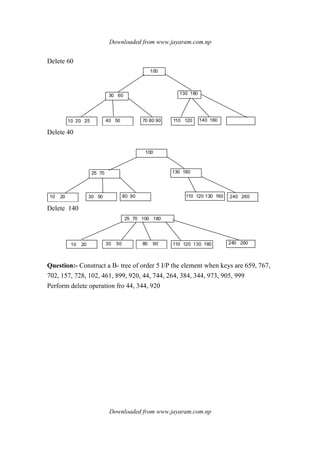
Insert 264 & 384
Insert 344
Insert 973 & 905 & 999
delete 44
delete 344 direct
Sorting:-
Sorting is storage of data in sorted order it can be in ascending or
descending order.
Type
Internal sort
External sort
In internal sorting data i.e. going to be sorted will be in many memory. In
external …….will be on auxiliary storage , tape floppy disk etc.
Sorting Technique:-
Insertion Sort:-
The insertion sort inserts each element in proper place if there are n-
element in array and we place each element of array at proper place in the
previously sorted element list.
Algorithm:-
Consider N elements in the array are
Pass 1 arr[0] is already sorted because of only one element.
Pass 2 arr[0] is inserted before or after arr[0]. So arr[0] & arr[i] are sorted.
Pass 3 arr[2] is inserted before arr[0], in between arr[0] & arr[1] or after
arr[0] . so arr[0] , arr[1] & arr [2] are sorted.
Pass 4 arr[3] is inserted in to it’s proper place in array arr[0], arr[1], arr[2],
arr[3] & are sorted.
…………………
……………………
Pass N arr[ N-1] is inserted in to it’s proper place in array arr[0], arr[1],
……. Arr[N-1]. So arr[0], arr[N-1] are sorted.](https://image.slidesharecdn.com/datastructureandalgorithm-141219101030-conversion-gate01/85/Data-structure-and-algorithm-dsa-74-320.jpg)
![Downloaded from www.jayaram.com.np
Downloaded from www.jayaram.com.np
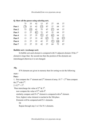
Q. Trace algo. With the given data using insertion sort.
82 42 49 8 92 25 59 52
Pass1 82 42 49 8 92 25 59 52
Pass 2 82 42 49 8 92 25 59 52
Pass 3 42 82 49 8 92 25 59 52
Pass 4 42 49 82 8 92 25 59 52
Pass 5 8 42 49 82 92 25 59 52
Pass 6 8 42 49 82 92 25 59 52
Pass 7 8 25 42 49 82 92 59 52
Pass 8 8 25 42 49 59 82 92 52
Pass 9 8 25 42 49 52 59 82 92
Selection Sort:-
Selection sort is the selection of an element & keepingit in sorted order. Let
us take an array arr[0]……..arr[N-1]. First find the position of smallest element
from arr[0] to arr [n-1]. Then interchange the smallest element from arr[1] to
arr[n-1], then interchanging the smallest element with arr[1]. Similarly, the
process will be for arr[0] to arr[n-1] & so on.
Algorithm:-
Pass 1:- search the smallest element for arr[0] ……..arr[N-1].
- Interchange arr[0] with smallest element
Result : arr[0] is sorted.
Pass 2:- search the smallest element from arr[1],……….arr[N-1]
- Interchange arr[1] with smallest element
Result: arr[0], arr[1] is sorted.
…………………
…………………
Pass N-1:-
- search the smallest element from arr[N-2] & arr[N-1]
- Interchange arr[N-1] with smallest element
Result: arr[0]…………. Arr[N-1] is sorted.](https://image.slidesharecdn.com/datastructureandalgorithm-141219101030-conversion-gate01/85/Data-structure-and-algorithm-dsa-75-320.jpg)
![Downloaded from www.jayaram.com.np
Downloaded from www.jayaram.com.np
Shell sort (Diminishing increment sort)
Shell sort is an improvement an insertion sort. In this case we take on itme
at a particular distance (increments) than we compare items which are far apart
and then sort them. After- words we decrease the increments & repeate this
process again. At last we take the increment one & sort them with insertion sort.
Procedure:-
Let us take an array from arr[0], arr[1]……… arr[N-1] & take the distance 5 (say)
for grouping together the items then in terms will grouped as:
First: arr[0], arr[5], arr[10],……….
Second: arr[1], arr[6], arr[11],………
Third: arr[1], arr[7], arr[12],……..
Fourth: arr[9], arr[8], arr[13]…….
We can see that we have to make the list equal to the increments & it will
cover all the items from arr[0]………arr[N-1].
First sort this list with insertion sort then decrease the increments & repeat this
process again.
At ht end, list is maintained with increment 1 & sort them with insertion sort.
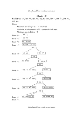
Question:- Show all the passes using shell sort with following list:-
75 35 42 13 87 27 64 57
Soln
:-
Consider increments 5
Pass1: 75 35 42 13 87 27 64 57
Pass 2 27 35 42 13 87 75 64 57
Pass 3 13 35 42 27 57 75 64 87
⇒ 13 27 35 42 57 64 75 87](https://image.slidesharecdn.com/datastructureandalgorithm-141219101030-conversion-gate01/85/Data-structure-and-algorithm-dsa-80-320.jpg)
![Downloaded from www.jayaram.com.np
Downloaded from www.jayaram.com.np
Explanation:-
Binary Tree sort:-
Create binary search tree.
Find in order traversal of binary tree.
Question:-
19 35 10 12 46 40 6 90 3 8
19
10
6
3
8
12
35
46
40
90
[do step by step]
In order traversal
3 6 8 10 12 19 35 40 46 90
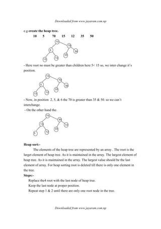
Heap Sort:-
Heaps:-
A heap is a binary tree that satisfied the following propertiers:-
→ shape property
→ Order property.
By the shape property we mean that heap must be a complete binary tree
where as by order property we mean that for every node in the heap the value store
in the heap node is greater than or equal to the value to the value an each of its’
children. A heap that satisfied this property is known as max heap.
However, If the order property is such that for every node. In the heap the
value stored in that node is less than or equal to the value in each of it’s children.
That heap is known as minimum heap.](https://image.slidesharecdn.com/datastructureandalgorithm-141219101030-conversion-gate01/85/Data-structure-and-algorithm-dsa-81-320.jpg)
![Downloaded from www.jayaram.com.np
Downloaded from www.jayaram.com.np
72
64
56
32
65
54
46
29 48 arr[8]arr[7]
arr[9]
arr[4]
arr[1]
arr[0]
arr[ 2]
arr[6]
arr[ 5]
72 64 65 56 32 46 54 29 48
0 1 2 3 4 5 6 7 8
arr
Step:-1 Root node is delete and this root node is replaced by last node and
the previous value of root node is placed in proper place in array.
48
64
29
12
65
46
54
56
4 8 64 65 56 3 2 5 4 2 9 72
Here, root node is less than 65. so we interchange the position to make heap tree.
65
64 54
56 32 46 48
29
Again , 48< 54
65
64 54
56 32 46 48
29
Now, which is in Heap tree form.
6 5 6 4 5 4 5 6 3 2 4 6 4 8 29 72
Again , delete root node & put 29 in root node.
2 9 6 4 5 4 5 6 3 2 3 2 4 6 48 6 5 7 2
2 9 6 4 5 4 5 6 3 2 3 2 4 6 48 6 5 7 2
6 5 6 4 5 4 5 6 3 2 4 6 4 8 29 72](https://image.slidesharecdn.com/datastructureandalgorithm-141219101030-conversion-gate01/85/Data-structure-and-algorithm-dsa-83-320.jpg)
![Downloaded from www.jayaram.com.np
Downloaded from www.jayaram.com.np
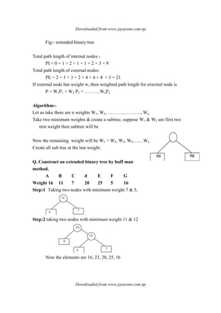
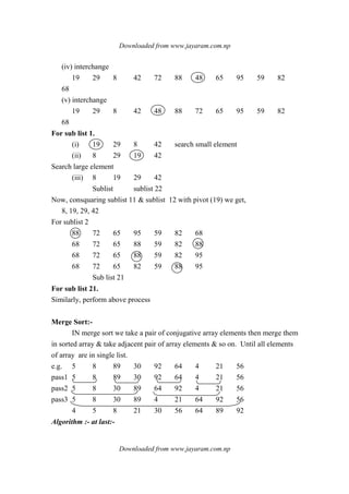
Radix sort:-
In radix sort, we sort the item in terms of it’s digits. If we have list of nos.
then there will be 10 parts from 0 to 9 because radix is 10.
Algo
consider the list n digit of nos, then there will be 10 parts from 0 to 9.
in the first pass take the nos in parts on the basis of unit digits.
In the second pass the base will be ten digit.
Repeat similarly for n passes for n digits.
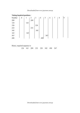
Show all the passes using radix sort.
233 124 209 345 498 567 328 163
Pass 1
Numbers [0] [1] [2] [3] [4] [5] [6] [7] [8] [9]
233 233
124 124
209 209
345 345
498 498
567 567
328 328
163 163
Pass 2
233 163 124 345 567 498 328 209
Number [0] [1] [2] [3] [4] [5] [6] [7] [8] [9]
233 233
163 1 163
124 124
345 345
567 567
498 498
328 328
209 209
209, 124, 328, 233, 345, 163, 567, 498.](https://image.slidesharecdn.com/datastructureandalgorithm-141219101030-conversion-gate01/85/Data-structure-and-algorithm-dsa-84-320.jpg)
![Downloaded from www.jayaram.com.np
Downloaded from www.jayaram.com.np
Chapter – 9
Searching
Definition:-
Searching is used to find the location whether element is available or not.
There are various kinds of searching techniques.
sequential search:-
simplest technique for searching on unordered table for particular record is to
scan each entry in sequential manner until the desired record is found.
If search is successful then it will return the location of element otherwise it
will return failene notification.
Consider, sequential search in array.
Arr [0] [1] [2] [3] [4] [5] [6]
10 20 30 40 50
Algorithm:-
Put a unique value at the end of array. Then.
(i) index =0
(ii) scan each element of array one by one.
(iii) (a) If match occurs then return the index value.
(b) otherwise index = index +1
(iv) Repeat the same process until unique value comes in scanning.
(v) Return the failure notification.
Consider sequential search in linked list.
Algorithm:-
Take a pointer of node type and initialize it with sort
Ptr = start
Scan each node of the linked list by traversing the list with the help of ptr.
Ptr = ptr → link;
If match occur then return.
Repeat the same process until null comes in scanning.
Return the failure notification.
Performance analysis:-](https://image.slidesharecdn.com/datastructureandalgorithm-141219101030-conversion-gate01/85/Data-structure-and-algorithm-dsa-86-320.jpg)
![Downloaded from www.jayaram.com.np
Downloaded from www.jayaram.com.np
Number of key comparison taken to find a particular record
Average case : (n+1)/2
Warpe case: n+1
Best case:- if desired record is present in the 1st
position of search table i.e. only
one comparison is made.
Binary search:-
The sequential search situation will be in worse case i.e. if the element is at
the end of the list. For eliminating this problem one efficient searching technique
called binary search is used in this case.
the entries are stored in sorted array.
The element to be searched is compared with middle element of the array.
a. If it is less than the middle element then we search. It in the left portion
of the array.
b. If it is greater than the middle element then search will be in the right
portion of the array.
The process will be in iteration till the element is searched or middle element
has no left or right portion to search.
Algorithm:-
Binary search (K.N, x)
→ entries in ascending order.
(i) [initialize]
Start ← 0, end ← N
(ii) Perform search
Repeat through step (iv) while low ≤ high
(iii) [obtain index of mid point of interval]
Middle ← [ (start + end)/2]
(iv) Compare
If X<K (middle)
Then end ← middle -1
Else
If X>K(middle);](https://image.slidesharecdn.com/datastructureandalgorithm-141219101030-conversion-gate01/85/Data-structure-and-algorithm-dsa-87-320.jpg)
![Downloaded from www.jayaram.com.np
Downloaded from www.jayaram.com.np
Then start ← middle +1
Else
Write (“Successful search”)
Return (middle)
(v) [unsuccessful search]
Return (0)
Question:- Tress a Binary search algorithm I/P data:-
75, 151, 203, 275, 318, 489, 524, 591, 647, 727
Search Pop x = 275, 727, 725.
Soln
:- [0] [1] [2] [3] [4] [5] [6] [7] [8] [9]
75 151 203 275 318 489 524 591 647 727
Iteration:1
Start = 0 end = 9 middle =
4
2
90
=
+
Since middle element [4] = 318
Since, the middle element is greater than search element, so we assign,
Iteration:-2
Start = 0 end = 3 middle =
1
2
30
=
+
[0] [1] [2] [3] [4] [5] [6] [7] [8] [9]
75 151 203 275 318 489 524 591 647 727
151 < 275
Now,
Start = middle + 1 = 2 end = 3
Iteration:- 3
[0] [1] [2] [3] [4] [5] [6] [7] [8] [9]
75 151 203 275 318 489 524 591 647 725
203 < 275 end = 3
Iteration :- 4](https://image.slidesharecdn.com/datastructureandalgorithm-141219101030-conversion-gate01/85/Data-structure-and-algorithm-dsa-88-320.jpg)
![Downloaded from www.jayaram.com.np
Downloaded from www.jayaram.com.np
Middle =
3
2
33
=
+
275 = 275
Middle [3] = 275
For 725
[0] [1] [2] [3] [4] [5] [6] [7] [8] [9]
75 151 203 275 318 469 524 591 647 727
Iteration:-1
Start = 0 end = 9 middle =
4
2
90
=
+
725> 318
Iteration:-2
Start = 5 end = 9 middle =
7
2
95
=
+
[0] [1] [2] [3] [4] [5] [6] [7] [8] [9]
75 151 203 275 318 489 524 591 647 727
725 < 591
Iteration:-3
Start = 8 end = 9 middle =
8
2
98
=
+
[0] [1] [2] [3] [4] [5] [6] [7] [8] [9]
75 151 203 275 318 489 524 591 647 727
725 < 647
Iteration:- 4
Start = 9 end = 9 middle =
9
2
99
=
+
[0] [1] [2] [3] [4] [5] [6] [7] [8] [9]
75 151 203 275 318 489 524 591 647 727
725 < 727
Binary search tree:- (BST)](https://image.slidesharecdn.com/datastructureandalgorithm-141219101030-conversion-gate01/85/Data-structure-and-algorithm-dsa-89-320.jpg)
![Downloaded from www.jayaram.com.np
Downloaded from www.jayaram.com.np
Algorithm:-
[initialize]
Read (no)
Root node content = 0
Right subtree = NULL
Left sub tree = NULL
while there is data
Do
Begin
Read(no)
compare no. with the content of root.
Repeat
If match then declare duplicates
Else
If no < root, then
Root = left sub tree root
Else
Root = right sub tree root.
Until
Duplicate found or (root = = NULL)
If(root = = NULL) then place it as root.
Application of BST:-
sorting a list
→ construct a BST &
→ Traverse in in order
For conversion prefix, infix & posfix expression.
→ construct a BST &
→ traverse in preorder, post order, inorder
Algorithm to build a binary search tree (BST) from post fix expression](https://image.slidesharecdn.com/datastructureandalgorithm-141219101030-conversion-gate01/85/Data-structure-and-algorithm-dsa-90-320.jpg)
![Downloaded from www.jayaram.com.np
Downloaded from www.jayaram.com.np
Inorder:-
Preorder:-
Post order:-
“Hashing”
Sequential search, binary search and all the search trees are totally
dependent on no. of element and may key comparisons are involved. Now, our
need is to search the element in constant time and loss key comparisons should be
involved.
Suppose all the elements are in array of size ‘N’. Let us take all the keys are
unique and in the rage ‘o’ to N-1. Now we are sorting the record in array based on
key, where array index and keys are same. Then we can access the record in
constant time and no key comparisons are involved.
Consider 5 records where keys are :-
9, 4, 6, 7, 2
The keys can be stored in array up
Arr [0] [1] [2] [3] [4] [5] [6] [7] [8] [9]
2 4 6 7 9
Here, we can see the record which has key value can be directly accessed through
array index.
In hashing key is converted into array index and records are kept in array.
In the same way for searching the record, key are converted into array index and
get the records from array.
For storing records:-
Key
↓
Generate array index
Key
↓
Stored the record on that array index.
For accessing record:-
Key
↓
Generate array index
Key
↓
Get the records from the array index](https://image.slidesharecdn.com/datastructureandalgorithm-141219101030-conversion-gate01/85/Data-structure-and-algorithm-dsa-92-320.jpg)
![Downloaded from www.jayaram.com.np
Downloaded from www.jayaram.com.np
A B
D
C
A B
C
D
A B
D
C
9
2
3
7
5
6
8
represents the node 2 & so on . similarly, column 1 represents node 1 & column 2
represents node 2 & so on. The entry of the matrix will be.
Arr[i][j] = 1 if there is an edge from node I to node j
= 0 if there is no edge from node I to node j.
A B C D outdegree
A 0 1 0 1 2
B 1 0 1 1 3
C 0 0 0 1 1
D 1 0 1 0 2
indegree 2 1 2 3
again,
For undirected graph:-
A B C D
A 0 1 1 1
B 1 0 1 1
C 1 1 0 1
D 1 1 1 0
It has no in degree & out degree because it has no direction of node.
Representation of weighted graph in matrix form:-
If graph has some weight on it’s edge then,
Arr[i][j] = weight on edge (if there is an edge from I to node j
= 0 (otherwise)
Weighted adjacency matrix
A B C D` out degree
A 0 2 0 8 10
B 3 0 4 7
C 0 0 0 5
D 9 0 6 0
Indegree =
Warshall Algorithm:-
Used for finding path matrix of a graph
Algorithm:-
Initialize
P ← A](https://image.slidesharecdn.com/datastructureandalgorithm-141219101030-conversion-gate01/85/Data-structure-and-algorithm-dsa-104-320.jpg)
![Downloaded from www.jayaram.com.np
Downloaded from www.jayaram.com.np
A B
D
C
[perform a pass]
Repeat through step 4 fro K = 1, 2, ……….n
process row]
Repeat step 4 for I = 1, 2, ………..n
process columns]
Repeat for j= 1, 2, ……….n
Pij U (Pik ∩Pkj)
[finish]
Return
Q:- From the given graph find out the path matrix by warshal algorithm.
A B C D`
A 0 1 0 1
P0 = B 1 0 1 1
C 1 1 0 1
D 1 1 1 0
Pij ∪ (Pik ∩ Pkj)
For k = 1
Pij ∪ (Pi1 ∩ P1j)
A B C D
A 1 0 1 0
P1 = B 1 1 1 1
C 0 0 0 1
D 1 1 1 1
Similarly taking k = 2 Pij = Pij ∪ (Pik ∩ Pkj)
Pij = Pij ∪ (Pi2 ∩ P2j)
A B C D`
A 1 1 1 1
P2 = B 1 1 1 1
C 0 0 0 1
D 1 1 1 1
Now taking k = 3,
A B C D`
A 1 1 1 1
P3 = B 1 1 1 1
C 0 0 0 1
D 1 1 1 1
Again taking k = 4](https://image.slidesharecdn.com/datastructureandalgorithm-141219101030-conversion-gate01/85/Data-structure-and-algorithm-dsa-105-320.jpg)
![Downloaded from www.jayaram.com.np
Downloaded from www.jayaram.com.np
A B C D`
A 1 1 1 1
P4 = B 1 1 1 1
C 1 1 1 1
D 1 1 1 1
Here, P0 is the adjency matrix & Pu is the path matrix of the graph.
Q:- Modified warshal’s algorithm:-
Warshall’s algoritham give the path matrix of graph. By modifying this
algorithm, we will find out the shortest path matrix Q. Qij represent the length of
shortest path from Vi to Vj. Here, we consider the matrices q0, q1, q2, ………. qn.
Thus, length of shortest path from Vi to Vj using nodes Vj,V2, ….Vn
Qk[i][j] =
∞ [i] there is no path from Vj to Vj using nodes V1, V2…………….
Vn
Procedures:-
→ In this algorithm length of 1st
path will be Qk-1 [i][j]
→ length of 2nd
path will be Qk-1 [i][j] + Qk-1 [i][j].
Now, select the smaller one from these two path length so value of
Qk [i][j] = Minimum [Qk-1 [i][j], Qk-1 [i][j] + Qk-1 [i][j] ]
Algorithm:-
→→→→ Q ←←←← A
- adjacency matrix with 0 replaced by ∞
→→→→ [Perform a pass]
- Repeat through step 4 for k = 1,2, ………..0.
→→→→ [process rows]
- Repeat step 4 fro j = 1,2, …………n
→→→→ [process column]
- Repeat for j = 1,2, ……….n
Qk [i][j] ← Min [Qk-1 [i][j], Qk-1 [i][j] + Qk-1 [i][j] ]
→→→→ [finish]
- Return
Case :-1
Qk [i][j] = ∞ & Qk-1 [i][j] + Qk-1 [i][j] = ∞
Then, Qk [i][j] =min (∞,∞ ) = ∞
Case :-2
Qk [i][j] = ∞ & Qk-1 [i][j] + Qk-1 [i][j] = b](https://image.slidesharecdn.com/datastructureandalgorithm-141219101030-conversion-gate01/85/Data-structure-and-algorithm-dsa-106-320.jpg)
![Downloaded from www.jayaram.com.np
Downloaded from www.jayaram.com.np
Then, Qk [i][j] =min (∞,b ) = b
Case :-3
Qk [i][j] = a & Qk-1 [i][j] + Qk-1 [i][j] = ∞
Then, Qk [i][j] =min (a,∞ ) = a
Case :-4
Qk [i][j] = a & Qk-1 [i][j] + Qk-1 [i][j] = b
Then, Qk [i][j] =min (a,b)
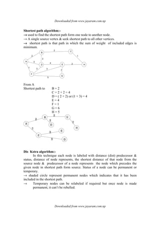
Traversal in graph:-
There are two efficient techniques for traversing the graph.
→ 1) depth first search (DFS)
→ 2) Breadth first search (BFS)
Difference between traversal in graph & traversal in tree or us
There is no 1st
node or root node in graph . Hence the traversal can start from
any node
In tree or list when we start traversing from the 1st
node, all the nodes are
traversed which are reachable from the starting node. If we want to
traverse al the reachable nodes we again have to select another starting
node for traversing the remaining nodes.
In tree or list while traversing we never encounter a node more then once but
while traversing graph,. There may be a possibility that we reach a node
more than once.
In tree traversal, there is only one sequence in which nodes are visited but in
graph for the same technique of traversal there can be different sequences
in which node can be visited.
Breadth first search:-
This technique uses queue for traversing all the nodes of the graph. In this
we take any node as a starting node than we take all the nodes adjacent to that
starting node. Similar approach we take for al other adjacent nodes which are
adjacent to the starting node & so on. We maintain the start up of the visited node
in one array so that no node can be traversed again.
Algorithm:-
[initialize]
Mark all vertex unvisited
begin with any node.
Insert it into queue (initially queue empty)
Remove node from queue.
append it to traversal list.
2 Mark it visited.](https://image.slidesharecdn.com/datastructureandalgorithm-141219101030-conversion-gate01/85/Data-structure-and-algorithm-dsa-107-320.jpg)
![Downloaded from www.jayaram.com.np
Downloaded from www.jayaram.com.np
4. insert al the unvisited or node snot an queue in to the queue.
2. Repeat step 3 to 5 until queue is empty.
3. [Finish]
Return.
1
2
8
3
5
6
7
8
3
3
5
5
5
6
6
6
7
7
7
7
Thus the traversal list is
1→ 2 → 8 → 3 → 4 → 5 → 6 → 7
Depth first Search:-
This technique uses stack for traversing all the nodes of the graph in this
we take one as starting node then go to the path which is from starting node &
visit all the nodes which are in that path. When we reach at the last node then we
traverse another path starting from that node. If there is no path in the graph from
the last node then it returns to the previous node in the path & traverse another &
so on.
Algorithm:-
1
*
2 8 3
2
*
1 4 5
3 1
*
6
*
7
4
*
2
*
8
5 2 8
6
*
3 8
7
*
3
*
8
8
*
4
*
5
*
1
*
6 7](https://image.slidesharecdn.com/datastructureandalgorithm-141219101030-conversion-gate01/85/Data-structure-and-algorithm-dsa-108-320.jpg)
![Downloaded from www.jayaram.com.np
Downloaded from www.jayaram.com.np
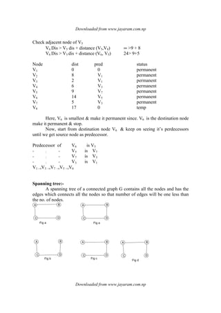
Procedure:-
→ Initially make source node permanent and make it the current working node
. al other nodes are node temporary.
→ Examine all the temporary neighbors of the current working nodes & after
checking the condition for minimum weight reliable the require node.
→ From all the temporary nodes find out the node which ahs minimum value
of distance, make the node permanent & now this is the current working
node.
→ Repeat step 2 & 3 until destination node is made permanent.
V3
V1
V4
V7
V8
V5 V6
V2
5
2
5
4
7
3
36
3
5
4 2
5
16
Let , V1 = source node
Node dist pred status
V1 0 0 permanent
V2 ∞ 0 temp
V3 ∞ 0 temp
V4 ∞ 0 temp
V5 ∞ 0 temp
V6 ∞ 0 temp
V7 ∞ 0 temp
V8 ∞ 0 temp
Check adjacent node of V3
V4 Dis > V3 dis + distance (V3,V4) 7<2+ 4 relable.
V7 Dis > V3sis + sistance (V3, V7) ∞> 2 + 3 relable
Node dist pred status
V1 0 0 permanent
V2 ∞ 0 temp
V3 ∞ 0 temp
V4 ∞ 0 temp
V5 ∞ 0 temp
V6] ∞ 0 temp
V7 ∞ 0 temp
V8 ∞ 0 temp](https://image.slidesharecdn.com/datastructureandalgorithm-141219101030-conversion-gate01/85/Data-structure-and-algorithm-dsa-111-320.jpg)
![Downloaded from www.jayaram.com.np
Downloaded from www.jayaram.com.np
Check adjacent node of V7
V4 Dis > V37 dis + distance (V7,V4) 7<2+ 4 relable.
V5 Dis > V7 sis + sistance (V7, V5) ∞> 2 + 3 relable V5
Node dist pred status
V1 0 0 permanent
V2 8 V1 temp
V3 2 V1 permanent
V4 6 V3 permanent
V5 9 V7 temp
V6] ∞ 0 temp
V7 5 V3 permanent
V8 ∞ 0 temp
Check adjacent node of V4
V5 Dis > V4 dis + distance (V4,V5) 9<6+9 leave.
Node dist pred status
V1 0 0 permanent
V2 0 V1 permanent
V3 2 V1 permanent
V4 6 V3 permanent
V5 9 V7 temp
V6] ∞ 0 temp
V7 5 V3 permanent
V8 ∞ 0 temp
Check adjacent node of V2
V6 Dis > V2 dis + distance (V2,V6) ∞>8 + 16 relable.
Node dist pred status
V1 0 0 permanent
V2 8 V1 permanent
V3 2 V1 permanent
V4 6 V3 permanent
V5 9 V7 permanent
V6] 24 0 temp
V7 55 V3 permanent
V8 ∞ 0 temp](https://image.slidesharecdn.com/datastructureandalgorithm-141219101030-conversion-gate01/85/Data-structure-and-algorithm-dsa-112-320.jpg)
![Downloaded from www.jayaram.com.np
Downloaded from www.jayaram.com.np
Here, A B C D is a spanning tree & D is the minimum spacing tree.
Node:- 1 2 3 4 5 6 7 8 9
Father:- 0 0 0 0 1 0 0 0 0
Step :2 = selected is 4 -5 wet = 3.
n1 = 4 root n1 = 4 n2 = 5 root n2 = 1
Roots are different, so edge is inserted.
Father [1] = 4
Node:- 1 2 3 4 5 6 7 8 9
Father:- 4 0 0 0 1 0 0 0 0
Step:- 4 edge selected is 3 – 6 wt = 5
n1 = 3 root – n1 = 3 n2= 6 root – n2= 6
father [6] = 3
roots are different so edge is inserted.
Node:- 1 2 3 4 5 6 7 8 9
Father:- 4 0 0 0 1 3 0 0 0
Step: 5 edge selected is 5-6 wt = 6
n1 = 5 root – n1 = 4 n2= 6 root – n2= 3
Roots are different so edge is inserted in spanning tree. Father of [3] = 4
Node:- 1 2 3 4 5 6 7 8 9
Father:- 4 0 0 0 1 3 0 0 0
Step: 6 edge selected is 3 -5 wt = 7
n1 = 3 root – n1 = 4 n2= 5 root – n2= 4
Roots are same so edge is not inserted i
Node:- 1 2 3 4 5 6 7 8 9
Father:- 4 0 4 0 1 3 0 0 0
Step: 7 edge selected is 2-5 wt = 8
n1 = 2 root – n1 = 2 n2= 5 root – n2= 4
Roots are different so edge is inserted Father of [4] = 2
Node:- 1 2 3 4 5 6 7 8 9
Father:- 4 0 4 2 1 3 0 0 0
Step: 8 edge selected is 1-2 wt = 9
n1 = 1 root – n1 = 2 n2= 2 root – n2= 32
Roots are same so edge is not inserted
Node:- 1 2 3 4 5 6 7 8 9
Father:- 4 0 4 2 1 3 0 0 0](https://image.slidesharecdn.com/datastructureandalgorithm-141219101030-conversion-gate01/85/Data-structure-and-algorithm-dsa-114-320.jpg)
![Downloaded from www.jayaram.com.np
Downloaded from www.jayaram.com.np
Step: 9 edge selected is 2-3 wt = 10
n1 = 2 root – n1 = 2 n2= 3 root – n2= 2
Roots are same so edge is not inserted
Node:- 1 2 3 4 5 6 7 8 9
Father:- 4 0 4 2 1 3 0 0 0
Step: 10 edge selected is 5-7 wt = 11
n1 = 5 root – n1 = 2 n2= 7 root – n2= 7
Roots are different so edge is inserted in spanning tree. Father of [7] = 2
Node:- 1 2 3 4 5 6 7 8 9
Father:- 4 0 4 2 1 3 2 0 0
Step: 11 edge selected is 5-8 wt = 12
n1 = 5 root – n1 = 2 n2= 8 root – n2= 8
Roots are different so edge is inserted in spanning tree. Father of [8] = 2
Node:- 1 2 3 4 5 6 7 8 9
Father:- 4 0 4 2 1 3 2 2 0
Step: 12 edge selected is 7-8 wt = 14
n1 = 7 root – n1 = 2 n2= 8 root – n2= 2
Roots are same so edge is not inserted
Node:- 1 2 3 4 5 6 7 8 9
Father:- 4 0 4 2 1 3 2 2 0
Step: 13 edge selected is 5- 9 wt = 15
n1 = 5 root – n1 = 2 n2= 9 root – n2= 9
Roots are different so edge is inserted in spanning tree. Father of [8] = 2
Node:- 1 2 3 4 5 6 7 8 9
Father:- 4 0 4 2 1 3 2 2 2
0 3
7
4 0 6
9
2
8
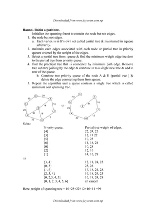
Since, minimum spacing tree should contain n-1 edges where n is the no. of nodes
in the graph. This graph contains nine nodes so after inserting 8 edges in the
spanning tree we will not examine other edges & stop the process.
Here, edge included in the spacing tree are (1, 5) (4, 5) (3, 6), (5, 6), (2, 5)
,(5, 7), (5, 8) & (5, 9) & weight of spanning tree = 2 + 3+ 5+ *+ 11+12 + 15
` = 62](https://image.slidesharecdn.com/datastructureandalgorithm-141219101030-conversion-gate01/85/Data-structure-and-algorithm-dsa-115-320.jpg)
![Downloaded from www.jayaram.com.np
Downloaded from www.jayaram.com.np
Greedy algorithm:-
Consider the problem of making changes Assume cosines of value 25φ
(quarter), 10φ & (dine), 5φ (nick) , & 1φ (penny) & suppose we want to return 63
φ in change, almost without thinking , we convert this amount to two quarters, one
dine & 3 pennies. Not only where we able to determine quickly lost of coins & the
correct value but we produce certain list of value with that coin.
The algorithm probably used to select the largest will whose value was not
greater than 63, & add it to the list of subtract it’s value from 63 getting 38[(63-
25) = 38]
We then select the largest coi9n whose value is not greater than 38 and add
it to the list & so one. According to this
63-25 = 38
38-25 = 13
13-10 = 3
3-1 =2
2-1 =1
1-1 = 0
This method of making charge is a greedy algorithm.
At any individual stage a greedy algorithm selects that option which is
locally optimum in same some particular sence. not that the greedy algorithm for
making change produces on over al optimum solution only because of special
properties of the coins. If the coins had value 1, 9 & 11 & we first select an 11
coin & then four 1 coins total of 5 coins.
We have seen several greedy algorithm such as Dijkstrals shortes path
algorithm & kruskal’s minimum cost spanning tree algorithm.
Kruskal’s algorithm is also greedy as it picks from remaining edges the
shortest among these that do not create a cycle.
/*Program of stack using Array */
# define max 5
Int top =-1;
Int stack_arr[Max];
Main()
{
Int choice;
While(1)
{
Printf(“1.psh”n”);
Printf(“2.pop”);
Printf(3. display”);
Printf( 4. quit”);
Printf(“Enter your choice”)](https://image.slidesharecdn.com/datastructureandalgorithm-141219101030-conversion-gate01/85/Data-structure-and-algorithm-dsa-117-320.jpg)
![Downloaded from www.jayaram.com.np
Downloaded from www.jayaram.com.np
Scanf(“%d”, choice);
Switch(choice)
{
Case 1:- psh();
Break;
Case 2: pop();
Break;
Case 3:- display()l;
Break;
Case 4: exit(4);
Default:
Printf(“wrong choice”);
}
}
}
Void push()
{
Int pushed_item;
If(top== (max -1)
Printf(“stack overflow”);
Else
{
Printf(“Enter that item to be pushed in stack”);
Scanf(“%d”, & pushed_item);
Top =top +1;
Stack_arr[top] = pushed_item;
}
}
Void pop()
{
If (top = =-1)
Printf(“stack uinderflow”);
Else
{
Printf(“popped element is %d”, stack_arr[top];
Top = top -1;
}
}
Void display()
{
Int I;
If(top == -1)
Printf(“Stack empty”);](https://image.slidesharecdn.com/datastructureandalgorithm-141219101030-conversion-gate01/85/Data-structure-and-algorithm-dsa-118-320.jpg)
![Downloaded from www.jayaram.com.np
Downloaded from www.jayaram.com.np
Else
{
Printf(“Stack element”);
For(i=top; I > = 0; i- -)
Printf(“%d”, stack_arr[i]);
}
}
/*Program of circular queue */
# define Max 5
Int cqueue_arr[Max];
Int front =-1;
Int rear =-1;
Main()
{
Int choice;
While (1)
{
Printf(“1. insert”);
Printf(2.delete”);
Printf(3.dispalay”);
Printf(4.quit”);
Printf(“Enter your choice”);
Scanf(“%d”, & choice);
Switch(choice)
{
Case 1: insert();
Break;
Case 2: del();
Break;
Case 3: display();
Break;
Case 4: exit(1);
Default:
Printf(“Wrong choice”);
}}}
Insert()
{
Int added_item;
If((front = = 0 & & rear = = Max -1)) || (front = = rear +1))
{
Printf(“Queue overflow”);
Return;](https://image.slidesharecdn.com/datastructureandalgorithm-141219101030-conversion-gate01/85/Data-structure-and-algorithm-dsa-119-320.jpg)
![Downloaded from www.jayaram.com.np
Downloaded from www.jayaram.com.np
}
If (front = = -1)
{
Front = 0;
Rear = 0;
}
Else
If (rear = = max -1)
Return =0;
}
else
Reae = rear +1;
Printf(“I/P element for insertion in queue”);
Scanf(“%d”, & added_item);
Cqueue_arr[rear] = added item;
Dle()
{
If(front ==-1)
{
Printf(“Queue underflow”);
Return;
}
Printf(“Element deleted from queue is %d”, cqueue_arr[front]);
If (front == rear)
{
Front =-1;
Rear =-1;
}
Else
If(front = max-1)
Font =0;
Else
Front = front +1;
}
Display()
{
Int fornt _pos = front; rear_pos = rear;
If (front == -1)
{
Printf(“queue is empty”);
Return;
}
Printf(“Queue elements”);](https://image.slidesharecdn.com/datastructureandalgorithm-141219101030-conversion-gate01/85/Data-structure-and-algorithm-dsa-120-320.jpg)
![Downloaded from www.jayaram.com.np
Downloaded from www.jayaram.com.np
If(front_pos<=rear_pos)
While(front_pos<=rear_pos)
{
Printf(%d”, cqueue_arr[front_pos]);
Front_pos + +;
}
Font_pos= 0;
While (front_pos<= rear_pos]);
Front_pos =0;
Whiel(frot_pos<=rear_pos)
{
Printf(%d”, cqueue arr[front_pos]);
Front_pos ++;
}}}
Output:-
1. insert
delete
display.
quit
enter Your choice:-1
input the element for insertion in queue 7
insert. 2. delete. 3. delete. 4. quit
enter your choice 1. input = 8
“ input = 9
+ input = 10
“ input = 11
# Define Max 5
Int deque_arr[max];
Int left =-1;
Int right =-1;
Main()
{
Int choice;
Printf(“1. I/P restricted dequeue”);
Printf(“2. O/P restricted dequeue”);
Printf(“Enter your choice”);
Scanf(“%D”, & choice);
Switch(choice)
{
Case 1: input_que();](https://image.slidesharecdn.com/datastructureandalgorithm-141219101030-conversion-gate01/85/Data-structure-and-algorithm-dsa-121-320.jpg)
![Downloaded from www.jayaram.com.np
Downloaded from www.jayaram.com.np
Right =0;
Else
Right = right +1;
Printf(“I/P the element for adding in queue”);
Scanf(“%d”, & added_item);
Deque_arr[right] = added_item;
}
Insert_lfet()
{
Int added_item;
If(left== 0&& right = max -1) || (left = right +1));
{
Printf(“Queue overflow”);
Return;
}
If(left ==-1
{
Left = 0;
Right =0;
}
Else
If(left = 0)
Left = max -1;
Else
Left = left-1;
Printf(“I/P thelement for adding”);
Scanf(“%d”, & added_item);
Deque_arr(left) = added_item;
}
Delete_left()
{
If(left ==-1)
{
Printf(“Queue underflow”):
Return;
}
Printf(“Element deleted from queue is %d”, deque_arr[left]);
If(left == right)
{
Left =-1;
Right =-1;
}
Else](https://image.slidesharecdn.com/datastructureandalgorithm-141219101030-conversion-gate01/85/Data-structure-and-algorithm-dsa-123-320.jpg)
![Downloaded from www.jayaram.com.np
Downloaded from www.jayaram.com.np
If()left== max-1)
Left =0;
Eles
Left = left +1;
}
Delete_right()
{
If(left ==-1)
{
Printf(“Queue under flow”);
Return;
}
Printf(“Element deleted from queue is %d”, deque_arr[right]);
If(left = = right)
{
Left = -1;
Right =-1;
}
Else
If(right = =0)
Right = max -1;
Else
Right = rightg -1;
}
Display_queue()
}
Program of list using array
#defince Max 10
Int arr[max];
Int n;
Main()
{
Int choice, item_pos;
While(1)
{
Print(“1. input list”);
Printf(“2. insert”);
Printf(“3. search”);
Printf(“4. display”);
Printf(“5. quit”);
Printf(“Enter your choice”);](https://image.slidesharecdn.com/datastructureandalgorithm-141219101030-conversion-gate01/85/Data-structure-and-algorithm-dsa-124-320.jpg)
![Downloaded from www.jayaram.com.np
Downloaded from www.jayaram.com.np
Scanf(“%d”, & choce);
Switch(choice)
{
Case 1:
Printf(“Enter the no. of element to be inserted”);
Scanf(“%d”, &n)
Input(n);
Break;
Case 2:
Break;
Case 3. insert();
Break;
Case 3: printf(“Enter elements to be serched”);
Scanf(“%d”, & item);
Pos = search(item);
If(p0os>=1)
Printf(“%d found at postion %d”, item, pos);
Else
Printf(“element not found”);
Break;
Case 4:
Del();
Break;
Case 5: display();
Break;
Case 6: exit();
Break;
Default:
Print(“Wrong choice”);
}}}
Input()
{
Int I;
For (I =0; i<n; i++)
{
Printf(“I/P value for element %d”,j+1);
Scanf(%d”, &arr[i]);
}}
Int search *(int item)
{
Int I;
For (I =0; i<n;i++)
{](https://image.slidesharecdn.com/datastructureandalgorithm-141219101030-conversion-gate01/85/Data-structure-and-algorithm-dsa-125-320.jpg)
![Downloaded from www.jayaram.com.np
Downloaded from www.jayaram.com.np
If (item == arr[i])
Return(i+1);
}
Return(0) /*if element not found */
}
Insert ()
{
Int temp, item, position;
If(n == max)
{
Printf(“list overflow”);
Return;
}
Printf(“enter positionfor insertion”)
Scanf(“%d”, & position);
Printf(“Enter the value”);
Scanf(“%d”, & item);
If position > n+1)
{
Printf(“Enter position less than or equal to n+1);
Return;
}
If position = n+1;
}
Arr[n] = item
n = n+1
return;
}
/*insertion in between */
Temp = n-1;
While (tem> = posiotn-1)
{
Arr[tem +1] = arr[temp];
Temp --;
}
Arr[position -1] = item;
n = n+1;
}
Del()
{
Int tem , position, item;
If(n==0)
{](https://image.slidesharecdn.com/datastructureandalgorithm-141219101030-conversion-gate01/85/Data-structure-and-algorithm-dsa-126-320.jpg)
![Downloaded from www.jayaram.com.np
Downloaded from www.jayaram.com.np
Printf(“list underflow”);
Return;
}
Printf(“Enter the element to be deleted”);
Scanf(“%d”, & item)
If (item = arr[n-1])
{
N = n-1;
Retun;
}
Position = search (item);
If (position == 0)
{
Printf(“Element not present in array”);
Return;
}
//Deletion in between
Temp = position -1;
While (tem<=n-1)
{
Arr[temp] = arr[temp +1];
Temp ++
{
N = n-1;
}
Display()
{
Int I;
If (n = = 0)
{
Printf(“List is empty”);
Return;
}
For (I =0; i<n; i++)
Printf(“value at position % %d”, i+1, arr[i]);
}
/* program of single linked list */
#include <stdio.h>
#include<malloc.h>
Struct node
Int info;](https://image.slidesharecdn.com/datastructureandalgorithm-141219101030-conversion-gate01/85/Data-structure-and-algorithm-dsa-127-320.jpg)