Downloaded 124 times


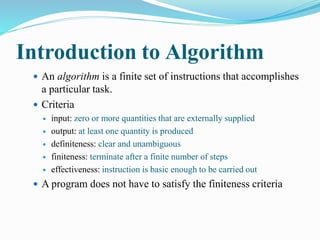
![[Cont…]
Representation
A natural language, like English or Chinese.
A graphic, like flowcharts.
A computer language, like C.
Algorithms + Data structures = Programs [NiklusWirth]](https://image.slidesharecdn.com/datastructureandalgorithm-141107231244-conversion-gate01/85/Data-structure-and-algorithm-5-320.jpg)
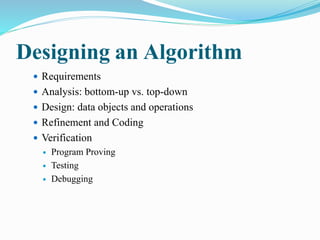

![[Cont…]
Since an algorithm's performance time may vary with
different inputs of the same size, one commonly uses
the worst-case time complexity of an algorithm, denoted
as T(n), which is defined as the maximum amount of time
taken on any input of size n. Time complexities are
classified by the nature of the function T(n). For instance,
an algorithm with T(n) = O(n) is called a linear time
algorithm, and an algorithm with T(n) = O(2n) is said to be
an exponential time algorithm.](https://image.slidesharecdn.com/datastructureandalgorithm-141107231244-conversion-gate01/85/Data-structure-and-algorithm-10-320.jpg)

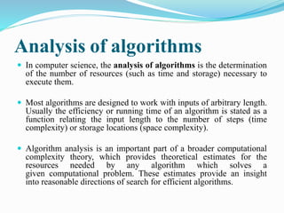
![Pointer Variable[Cont…]
Pointers are declared with the use of the asterisk ( *). In
the example
int *foo;
float *bar;
Here, foo is declared as a pointer to an integer, and bar is
declared as a pointer to a floating point number.](https://image.slidesharecdn.com/datastructureandalgorithm-141107231244-conversion-gate01/85/Data-structure-and-algorithm-15-320.jpg)
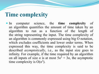
![Pointer Variable[Cont…]
To make a pointer variable point at some other variable,
the ampersand operator is used. The ampersand operator
returns the address of a variable's value; that is, the place
in memory where the variable's value is stored. Thus:
int *foo;
int x= 5;
foo= &x;
It makes the pointer foo ``point at'' the value of x (which
happens to be 5).](https://image.slidesharecdn.com/datastructureandalgorithm-141107231244-conversion-gate01/85/Data-structure-and-algorithm-16-320.jpg)
![Pointer Variable[Cont…]
This pointer can now be used to retrieve the value
of x using the asterisk operator. This process is called de-referencing.
The pointer, or reference to a value, is used to
fetch the value being pointed at. Thus:
int y;
y= *foo;
It sets y equal to the value pointed at by foo. In the
previous example, foo was set to point at x, which had the
value 5. Thus, the result of dereferencing foo yields 5,
and y will be set to 5.](https://image.slidesharecdn.com/datastructureandalgorithm-141107231244-conversion-gate01/85/Data-structure-and-algorithm-17-320.jpg)


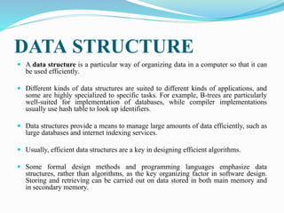
The document discusses data structures and algorithms. It defines a data structure as a particular way of organizing data in a computer so that it can be used efficiently. Common data structures include arrays, stacks, queues, linked lists, trees, heaps, and hash tables. An algorithm is defined as a finite set of instructions to accomplish a particular task. Analyzing algorithms involves determining how resources like time and storage change with input size. Key considerations in algorithm design include requirements, analysis, data objects, operations, refinement, coding, verification, and testing.