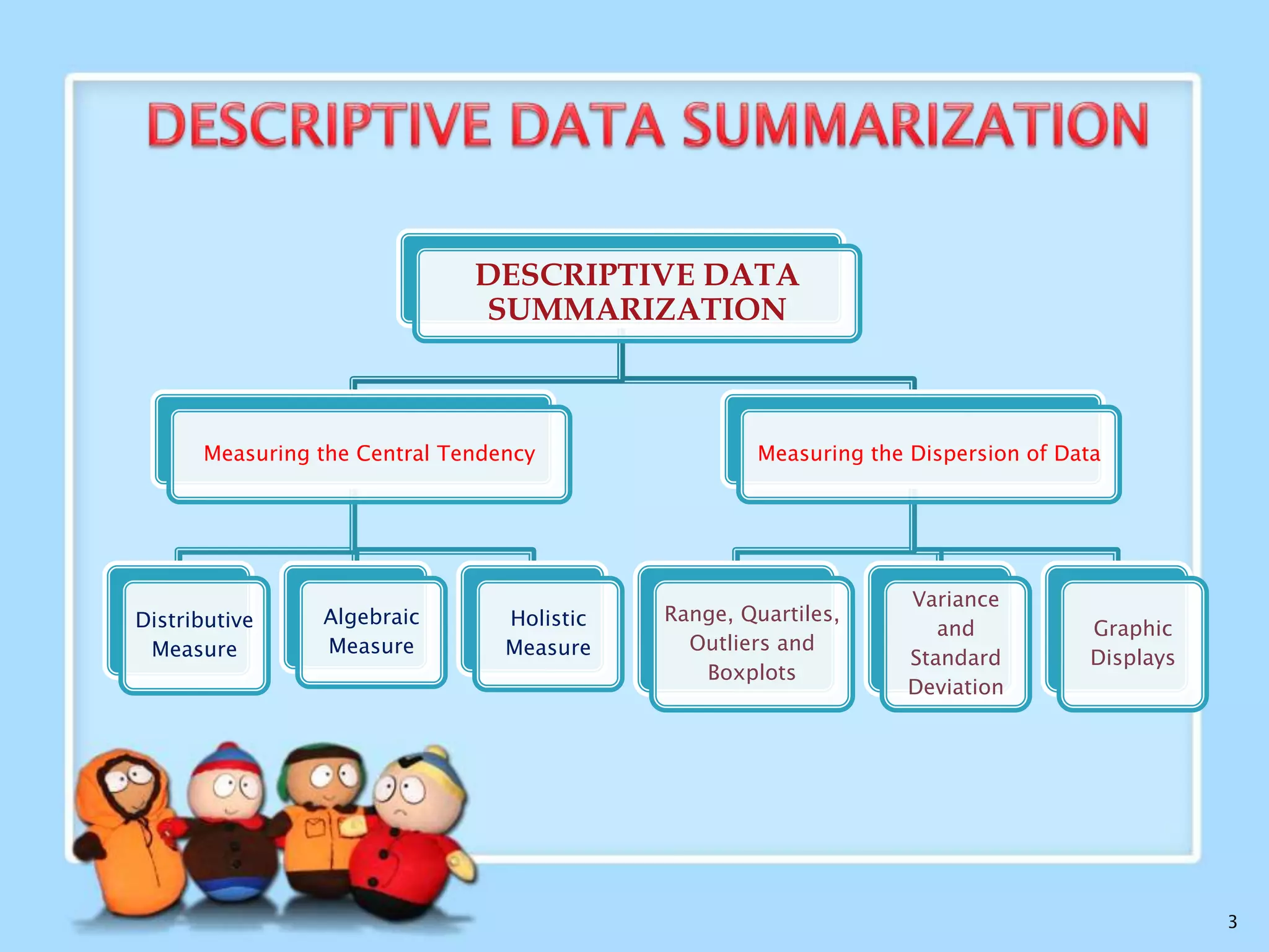
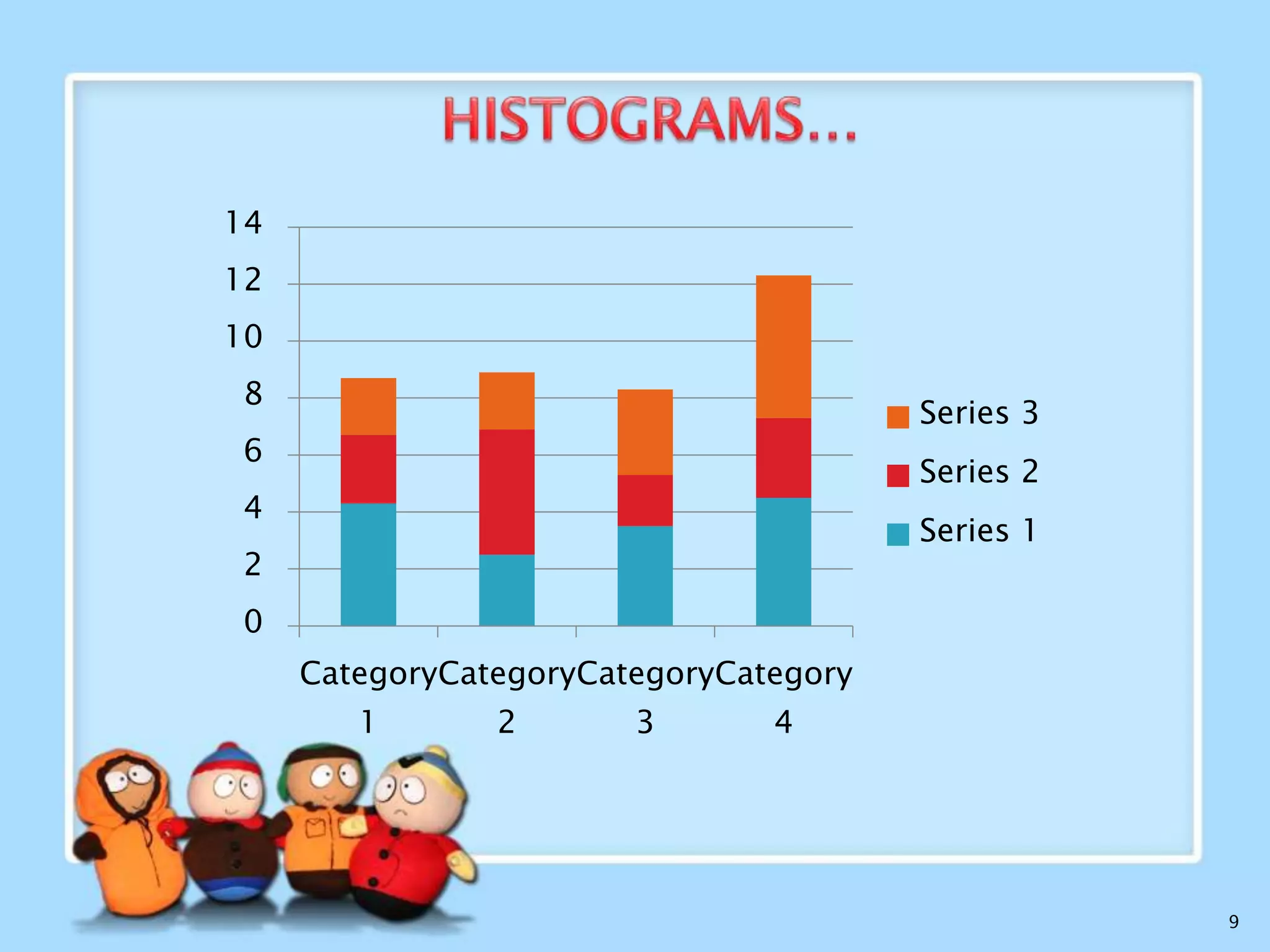
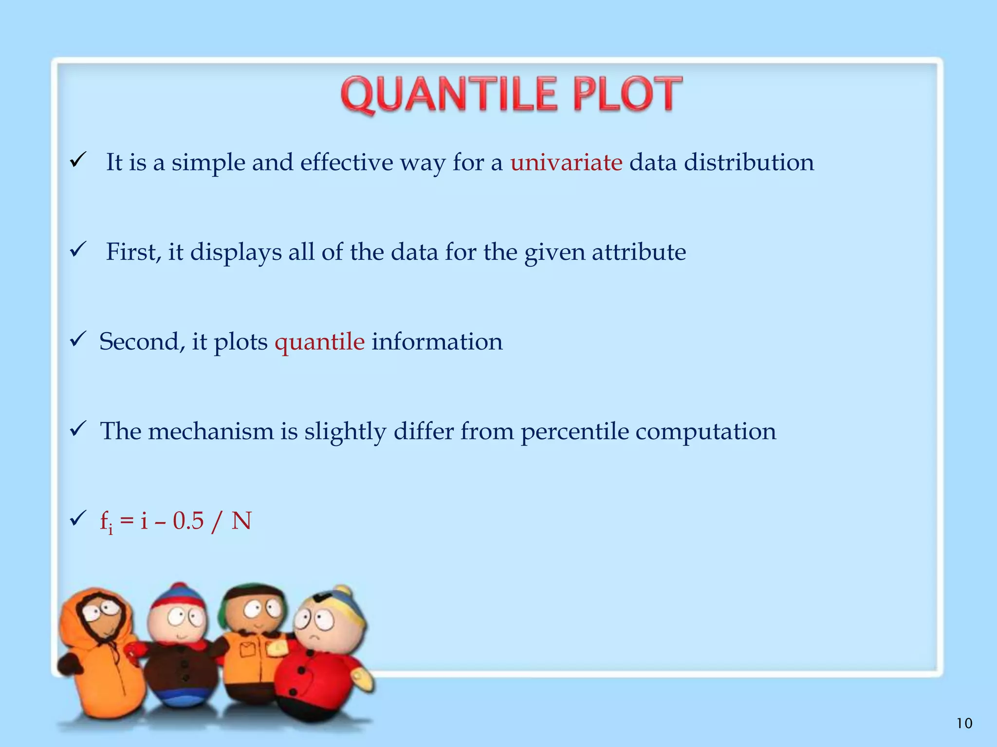
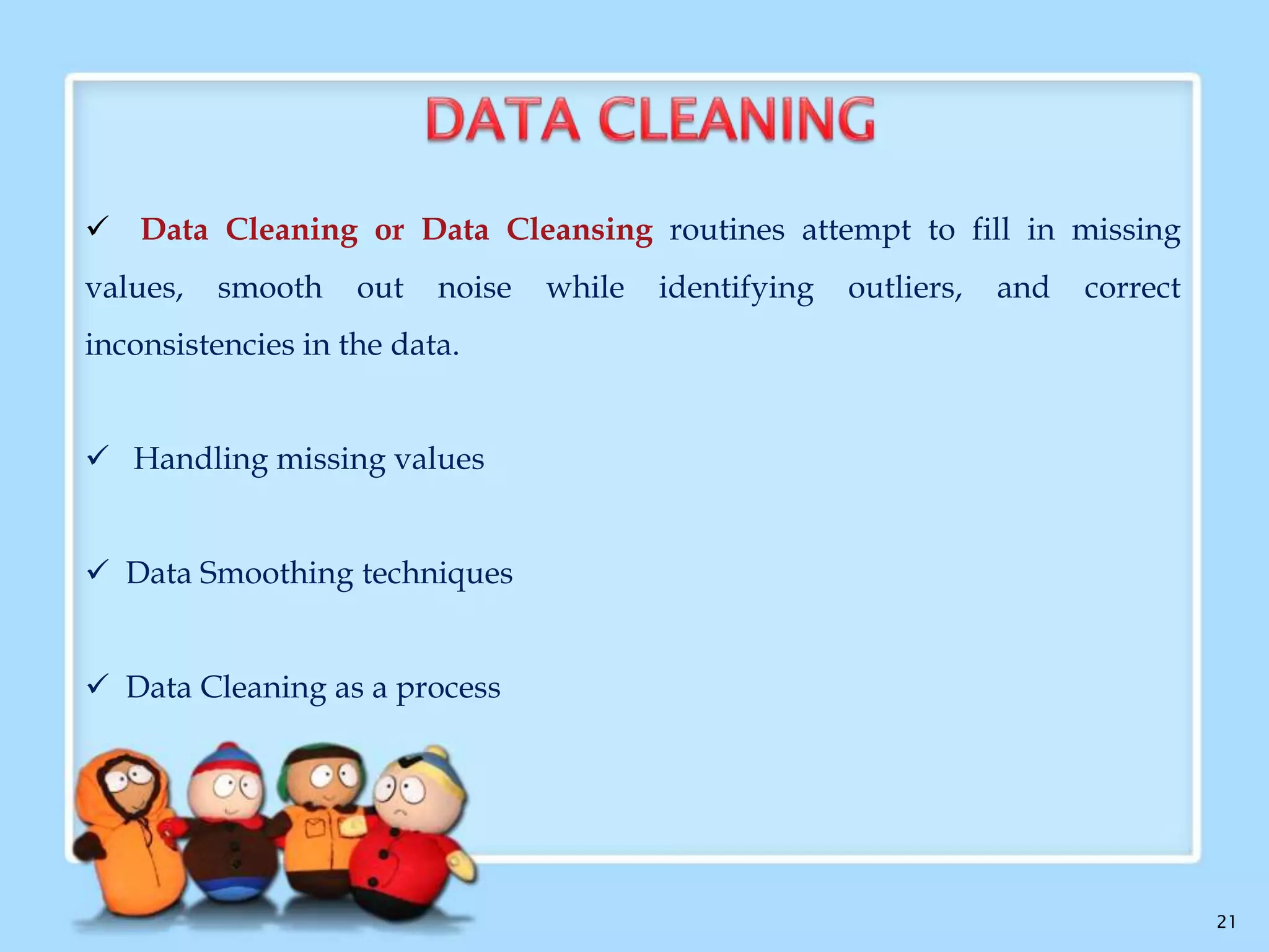
The document discusses descriptive data summarization techniques for data cleaning and preprocessing. It describes common issues with real-world data including missing values, noise, and inconsistencies. Common techniques for data cleaning are then presented, such as data cleaning, integration, transformation, and reduction. Methods for handling missing values, smoothing noisy data, and resolving inconsistencies are outlined. Finally, descriptive statistical techniques for summarizing data distributions are reviewed, including measures of central tendency, dispersion, and graphical displays like histograms and scatter plots.

1. 1

2. Data in the real world is dirty
incomplete: lacking attribute values, lacking certain attributes of
interest, or containing only aggregate data
e.g., occupation=― ‖
noisy: containing errors or outliers
e.g., Salary=―-10‖
inconsistent: containing discrepancies in codes or names
e.g., Age=―42‖ Birthday=―03/07/1997‖
e.g., Was rating ―1,2,3‖, now rating ―A, B, C‖
e.g., discrepancy between duplicate records
2

3.  Data Cleaning / Data Cleansing
Fill in missing values, smooth noisy data, identify or
remove outliers, and resolve inconsistencies
 Data Integration
Integration of multiple databases, data cubes, or files
 Data Transformation
Normalization and aggregation
 Data Reduction
Obtains reduced representation in volume but produces
the same or similar analytical results
3

4. DESCRIPTIVE DATA
SUMMARIZATION
Measuring the Central Tendency
Distributive
Measure
Algebraic
Measure
Holistic
Measure
Measuring the Dispersion of Data
Range, Quartiles,
Outliers and
Boxplots
Variance
and
Standard
Deviation
Graphic
Displays
4

5. The variance of N observations, x1, x2, ....xN is
1
2 =
N
N
( xi x)
i1
2
1
N
2
i
x
1
( xi )2
N
5

6. Where
x
is the mean value of observations
The Standard deviation is 
The  of the observations is the square root of the
variance,  2
6

7. The basic properties of the standard deviation ,
  measures spread about the mean and should be used only
when the mean is chosen as the measure of center
  = 0 only when there is no spread, that is, when all
observations have the same value. Otherwise  > 0
7

8. 
Apart from the bar charts, pie charts and line graphs, there
are other popular types of graphs for the display of data
summaries and distributions.
Histograms
Quantile plots
q-q plots
Scatter plots
Curves
8

9.  Plotting histograms, or frequency histograms, is a graphical method
for summarizing the distribution of a given attribute.
 A histogram for an attribute A partitions into subsets or buckets.
 The width of each bucket is uniform
 Each bucket is represented by a rectangle
 The resulting graph is referred to as Bar chart
9

10. 14
12
10
8
6
4
2
0
Series 3
Series 2
Series 1
10

11.  It is a simple and effective way for a univariate data distribution
 First, it displays all of the data for the given attribute
 Second, it plots quantile information
 The mechanism is slightly differ from percentile computation
 fi = i – 0.5 / N
11

12. 12

13.  A quantile-quantile plot, or q-q plot graphs the quantiles of one
variate distribution against the corresponding quantiles of another
 It is a powerful visualization tool that allows the user to view
whether there is a shift in going from one distribution to another.
13

14. 6
5
4
3
Series 1
2
Series 2
1
Series 3
0
Category Category Category Category
1
2
3
4
14

15.  A Scatter plot used for determining if there appears to be a
relationship, pattern, or trend between two numerical attributes
 To construct a scatter plot, each pair of values is treated as a pair of
coordinates in an algebraic sense and plotted as points in the plane
 Bivariate data to see clusters of points and outliers or correlation
relationships
15

16. Y-Values
3.5
3
2.5
2
1.5
Y-Values
1
0.5
0
0
1
2
3
16

17. Y-Values
3.5
3
2.5
2
1.5
Y-Values
1
0.5
0
0
1
2
3
17

18. Y-Values
3.5
3
2.5
2
1.5
Y-Values
1
0.5
0
0
1
2
3
18

19.  It is another graphic aid that adds a smooth curve to a scatter plot in order
to provide better perception of the pattern of dependence
 The word loess is short for ―local regression‖
 There are two values are needed that is smoothing parameter () and , the
degree of the polynomials that are fitted by regression
19

20. Y-Values
3.5
3
2.5
2
1.5
Y-Values
1
0.5
0
0
1
2
3
20

21.  Descriptive data summaries provide valuable insight into the
overall behavior of our data
 By helping to identify noise and outliers, they are especially useful
for data cleaning
21

22.  Data Cleaning or Data Cleansing routines attempt to fill in missing
values,
smooth
out
noise
while
identifying
outliers,
and
correct
inconsistencies in the data.
 Handling missing values
 Data Smoothing techniques
 Data Cleaning as a process
22

23. Many tuples have no recorded value for several attributes
Methods:
1. Ignore the tuple :
This is usually done when the class label is missing
It is not very effective
2. Fill in the missing value manually:
It is time-consuming and may not be feasible in large data set
3. Use a global constant to fill in the missing value:
Replace all missing attribute values by the same constant
23

24. 4. Use the attribute mean to fill in the missing value:
Use the mean value to replace the missing value for particular
attribute
5. Use the attribute mean for all samples belonging to the same class as the
given tuple:
if classifying customers according to credit_risk, replace the missing
value with the average income value for customers
6. Use the most probable value to fill in the missing value:
This may be determined with regression, inference-based tools using
a Bayesian formalism, or decision tree induction.
24

25.  Methods 3 to 6 bias the data. The filled-in value may not be correct
 Method 6 is a popular strategy to predict missing values
 By considering the other values of the other attributes in its estimation
of the missing value
 In some cases, a missing value may not imply an error in the data!
Ex: Phone number in some application form  NULL
25

26.  What is Noise?
 Noise is a random error or variance in a measured variable.
 Data Smoothing techniques:
Binning
Regression
Clustering
26

27.  Binning
first sort data and partition into (equal-frequency) bins then
one can smooth by bin means, smooth by bin median, smooth by bin
boundaries, etc.
 Regression
smooth by fitting the data into regression functions
 Clustering
detect and remove outliers
27

28. Combines data from multiple sources into a coherent store
 Schema integration:
Integrate metadata from different sources
 Entity identification problem:
Identify real world entities from multiple data sources,
e.g., Bill Clinton = William Clinton
 Detecting and resolving data value conflicts
For the same real world entity, attribute values from different
sources are different
28

29. Redundant data occur often when integration of multiple databases
Object identification: The same attribute or object may have
different names in different databases
Derivable data: One attribute may be a ―derived‖ attribute in
another table, e.g., annual revenue
Redundant attributes may be able to be detected by correlation analysis
Careful integration of the data from multiple sources may help
reduce/avoid redundancies and inconsistencies and improve mining
speed and quality
29

30. Smoothing: remove noise from data
Aggregation: summarization, data cube construction
Generalization: concept hierarchy climbing
Normalization: scaled to fall within a small, specified range
min-max normalization
z-score normalization
normalization by decimal scaling
30

31. 
Min-max normalization: to [new_minA, new_maxA]
v'
v minA
(new _ maxA new _ minA) new _ minA
maxA minA
◦ Ex. Let income range $12,000 to $98,000 normalized to [0.0, 1.0].
Then $73,000 is mapped to 73,600 12,000 (1.0 0) 0 0.716
98,000 12 ,000


Z-score normalization (μ: mean, σ: standard deviation):
v
A
v'
73,600 54 ,000
A
1.225
◦ Ex. Let μ = 54,000, σ = 16,000. Then
Normalization by decimal scaling
v
v'
10 j
16 ,000
Where j is the smallest integer such that Max(|ν’|) < 1
31

32. Why data reduction?
 A database/data warehouse may store terabytes of data
 Complex data analysis/mining may take a very long time to run on
the complete data set
Data reduction
Obtain a reduced representation of the data set that is much
smaller in volume but yet produce the same (or almost the same)
analytical results
Data reduction strategies
o Data cube aggregation:
o Dimensionality reduction — e.g., remove unimportant attributes
o Data Compression
o Numerosity reduction — e.g., fit data into models
o Discretization and concept hierarchy generation
32

33.  Data preparation or preprocessing is a big issue for both data
warehousing and data mining
 Discriptive data summarization is need for quality data preprocessing
 Data preparation includes,
 Data cleaning and data integration
 Data reduction and feature selection
 Discretization
 A lot a methods have been developed but data preprocessing still an active
area of research
33

34. 34