This document describes the development of an Aspen Custom Modeler simulation of a double stirred cell used to capture CO2 in a water-caustic potash solution. The simulation allows the user to specify inlet gas and liquid stream compositions and calculates changing molality and pressure over time as reactions reach equilibrium. Key aspects include defining component properties, calculating Henry's law constants, and using the Pitzer model to calculate activity coefficients as molalities change due to the kinetic and equilibrium reactions between CO2, water, and potash solution components.

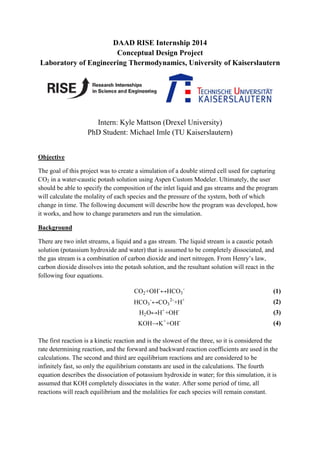
1. DAAD RISE Internship 2014
Conceptual Design Project
Laboratory of Engineering Thermodynamics, University of Kaiserslautern
Intern: Kyle Mattson (Drexel University)
PhD Student: Michael Imle (TU Kaiserslautern)
Objective
The goal of this project was to create a simulation of a double stirred cell used for capturing
CO2 in a water-caustic potash solution using Aspen Custom Modeler. Ultimately, the user
should be able to specify the composition of the inlet liquid and gas streams and the program
will calculate the molality of each species and the pressure of the system, both of which
change in time. The following document will describe how the program was developed, how
it works, and how to change parameters and run the simulation.
Background
There are two inlet streams, a liquid and a gas stream. The liquid stream is a caustic potash
solution (potassium hydroxide and water) that is assumed to be completely dissociated, and
the gas stream is a combination of carbon dioxide and inert nitrogen. From Henry’s law,
carbon dioxide dissolves into the potash solution, and the resultant solution will react in the
following four equations.
CO2+OH-
↔HCO3
-
(1)
HCO3
-
↔CO3
2-
+H+
(2)
H2O↔H+
+OH-
(3)
KOH→K+
+OH-
(4)
The first reaction is a kinetic reaction and is the slowest of the three, so it is considered the
rate determining reaction, and the forward and backward reaction coefficients are used in the
calculations. The second and third are equilibrium reactions and are considered to be
infinitely fast, so only the equilibrium constants are used in the calculations. The fourth
equation describes the dissociation of potassium hydroxide in water; for this simulation, it is
assumed that KOH completely dissociates in the water. After some period of time, all
reactions will reach equilibrium and the molalities for each species will remain constant.

2. Mattson 2
Explanation of the Code
Here are some general comments before going into line-by-line explanation. Double slash (//)
is used for commenting, the word “as” defines variables, and using “componentlist” will give
a value for that variable for each component (i.e. mole fraction, density, etc.). For adding
components, the user can upload a component list from an Aspen Property file, and the
component properties such as molecular weight or vapor pressure can be called from that file
into the code. “Fixed” variables like temperature will not change in the model, “Initial”
variables like molality will change in time when dynamic mode is implemented, and “Free”
variables like mole fraction will be calculated by the program. Additionally, the code must be
compiled before it can be run in steady state, initialization, or dynamic mode. More
information concerning the basics of Aspen Custom Modeler can be found in references one
and two, which are at the end of this report.
The outline below will describe in detail how each section works in the code, and screen-shots
from the code are below as well.
Lines 2-8: Default
• Default lines from Aspen Custom Modeler; they explain syntax for parameters,
variables, etc.
Lines 10-14: Ports
• Ports are what connect streams to the models, and in this case, connect the inlet liquid
and gas streams to the tank. There are also liquid and gas outlet streams, which can be
equated to the solution as it approaches equilibrium
• The port “Main” can be found under Port Types in Custom Modeling, and there the
flow rate, mole fraction, and other properties are defined
• In this code, G is for gaseous stream and L is for liquid stream
Lines 16-33: Tank Specs
• Defines tank temperature and pressure as well as physical parameters like liquid area,
height, and volume

3. Mattson 3
• Also defines component mole fractions and the gas constant R
• CO2 and N2 will have individually calculated partial pressures and the total pressure
will be calculated from them
Lines 35-49: Defining Component Properties
• Defines molecular weight, density, vapor pressure, Henry parameters, activity
coefficients, and diffusion coefficients for each component. The Henry coefficients are
calculated later using these parameters for each component i in component j
• Subsequently, all values except activity coefficient are called from the Aspen Property
file. The activity coefficient will be calculated using the Pitzer model, since the called
values have proven to be inaccurate for this system. The diffusion coefficient will be
called later in the program since it is dependent on mole fraction
Lines 51-53: Calculating Henry Constants
• The Henry constants for each combination of component i in component j are
calculated using the parameters previously called in the following equation:
kH , =Hparam1 ,
+
Hparam2 ,
T
+Hparam3 , * ln T +Hparam4 , *T+
Hparam5 ,
T2
(5)
• The only coefficients that are needed in this model are the coefficients of CO2 and N2
in water
Lines 55-72: Define Parameters for Calculating Pressures of CO2 and N2 using SRK Equation
of State

4. Mattson 4
• The Soave-Redlich-Kwong (SRK) Equation of State is used in this code to calculate
the pressure over the liquid solution
• Acentric factors as well as critical temperatures and pressures are defined and called
for each component, though the only ones needed are for CO2 and N2
o Note: The program will incorrectly report the critical temperatures and
pressures in C and Bar, they are actually K and Pascal respectively
• Reduced temperature, a, b, and alpha are defined for each gaseous component and will
be calculated later
Lines 74-81: Set Inlet Port Conditions
• Molar flow rate (F) and composition (Z) are defined for inlet gas and liquid streams.
The gas stream is N2/CO2 and the liquid stream is H2O/KOH
• These values for the inlet flow rates are based on 0.5m3
of gas and liquid each. The
volume was converted to molar flow rate using the following formula for each stream
(the liquid stream will be used as an example):
Vliquid*ρliquid,average
MWliquid,average
= nliquid (6)
• Here, ρ is the average liquid density, and MW is the average molecular weight
Lines 83-96: Set Solution Properties Prior to Reaction
• Inlet molar flow for inside the reactor is set by using the previously defined port
conditions
o Here it is assumed that KOH completely dissociates, so there is no KOH in the
solution, only K+
and OH-
ions
• The initial concentration values for HCO3
-
, CO3
2-
, and H+
are initial guesses, so any
value in a certain range will be fine, as long as it is above 0
o Note: In general, avoid using 0 in equations as this can lead to problems like
dividing by 0 when the program is doing iterations. Instead, use very small
values like 1E-10.

5. Mattson 5
• Molality is also defined here because the pressure of CO2 will depend on the changing
molality in the solution. Even though it is defined here, it will not be calculated until
later in the code
o Note also that molality is set as an initial value, so it will be the main variable
changing in time in this code
Lines 98-114: Calculating Pressure of CO2, N2, and total pressure
• Molar volume (Vm) is calculated for each gaseous component (CO2 and N2) by using
the changing molality in the liquid phase. By doing this, the pressure above the
solution will change as the molality in the solution changes
• The following equations are used in the SRK equation of state:
Tr, =
T
Tc
(7)
a =
0.427*R2
*Tc
2
Pc
(8)
b =
0.08664*R*Tc,
Pc,
(9)
α =(1+ 0.48508+1.55171ω - 0.15613ω 2
1- Tr, )
2
(10)
P =
R*T
Vm, -b
-
a *α
Vm, (Vm, +b )
(11)
• The total pressure is then calculated by summing the partial pressures of CO2, N2, and
the vapor pressure of water
Lines 116-124: Define Pitzer Model Constants

6. Mattson 6
• Constants are defined for the Pitzer model, which will calculate the activity
coefficients for each component on the molality basis. These include the number Pi,
Avogadro’s number, the electron charge, etc. These values will be used later in the
Pitzer equations.
Lines 126-138: Define and Call Binary Beta 0, Beta 1, and Ternary Mu Pitzer Parameters
• β(0)
and β(1)
are binary parameters and µ is a ternary parameter, all of which are used in
the Pitzer model. The beta parameters can be called from the Aspen Property file, and
the values for beta can be calculated in a similar manner as was done for the Henry
constants. However, the mu parameters cannot be called, but there are only eight
values that are not zero. To account for this, all values are set to zero and the eight
non-zero values are input manually via the output form. These eight values are taken
from the Aspen Property file as well.
• The beta and mu values are calculated later in the code using temperature dependent
correlations
Lines 140-149: Define Calculated Pitzer Parameters and Calculate Beta and Mu values
• Here, Z is the component charge, IonS is the ionic strength, Aphi is the Debye-Hückel
constant, and Bpitz is an osmotic coefficient which is depended on the beta values
• The following temperature dependent equations calculate β(0)
, β(1)
and µ:
β ,
(0)
= B0param1 ,
+
B0param2 ,
T
+
B0param3 ,
T2
(12)
β ,
(1)
= B1param1 ,
+
B1param2 ,
T
+
B1param3 ,
T2
(13)
µ , ,
= muparam1 , ,
+ muparam3 , ,
1
T
-
1
Tref
(14)
• In equation 14, Tref is 298.15K

7. Mattson 7
• Note: the binary and tertiary parameters are symmetric for all components, so βi,j = βj,i
and µi,j,k = µi,k,j = µj,i,k = µj,k,i = µk,i,j = µk,j,i
Lines 151-162: Calculate Pitzer Values and Activity Coefficients
• First, the charge for each component is called from Aspen Properties
• Next, the following equations are used to calculate the activity coefficients for each
component:
Aϕ=
1
3
2πNAρw
e2
4πϵ0ϵwkBT
1.5
(15)
I=
1
2
m
mo
z 2
(16)
B , =β ,
(0)
+
2β ,
(1)
α1
2I
1- 1+α1√I exp -α1√I (17)
ln γ (m)
= -Aϕzi
2 √I
1+b√I
+
2
b
ln 1+b√I !
+ 2
m
mo
B ,
#$
-
2z 2
α1
2I2 1- 1+α1√I+
α1
2
2
I exp -α1√I !
∗
m
mo
m
mo
β ,
1
#$#$
+3
m
mo
m
mo
µ , ,
#$#$
(18)
• Note: e in equation 15 is the charge of an electron, not the natural exponent
• Here, m stands for the molality of the species, and mo
is the standard molality, which
is set to 1mol/kg. This is used to make the summations be unitless.
• Since the molality of each species will be changing in time, the activity coefficient of
each species will be changing as well, since it is dependent on the individual and
overall molality of the solution. Eventually, as the molalities reach equilibrium, the
activity coefficients will approach equilibrium values as well

8. Mattson 8
Lines 164-174: Calculating Initial Concentrations in Solution
• Henry’s Law is used to calculate the initial concentration of CO2 and N2 in solution.
For all other species, the concentration is simply the incoming moles over the volume
of solution
Lines 176-179: Calculating Initial Mole Fractions
• For loop calculates mole fraction by dividing initial concentration of each component
over total concentration
Lines 181-199: Extents of Reaction
• Extents of reaction are created for each of the three reactions. These will be used in
conjunction with the kinetic and equilibrium equations. The general way to write
extent of reaction equations is shown below:
n ,final-n ,initial = υ *ξ (19)
o Here, ν is the stoichiometric coefficient for the component and ξ is the extent
of reaction for each equation; so the change in moles for any component is
equal to the sum of the extent of reactions multiplied by each stoichiometric
coefficient. An example for HCO3
-
is shown below based on the reactions on
page one:

9. Mattson 9
Vliquid* concHCO3
-
,final-concHCO3
-
,initial = ξ1
-ξ2 (20)
• The volume does not change very much since the solution is dilute, so the only things
that change in the system are the concentrations of each component
• Additionally, the outlet concentration and activity variables are created. The outlet
concentration is used here and the activity (molality basis) will be calculated and used
later.
Lines 201-206: Old Equilibrium Reaction One (Commented Out)
• This describes the following equilibrium reaction:
CO2+H2O ↔ HCO3
-
+H+
(21)
• However, this equation is not used in the calculations because the kinetic equation
(number one) is much slower than this one. This equation is kept in the code solely for
referencing purposes
Lines 208-216: Kinetic Reaction
• This creates the forward, backward, and equilibrium coefficients for the kinetic
reaction. The forward and backward constants are calculated using an Arrhenius
equation, and the equilibrium constant is calculated once the other two are known
kforward or kbackward = k0*exp
-Ea
RT
(22)
kequilibrium =
kforward
kbackward
(23)
o Here, k0 is a pre-exponential factor, Ea is the activation energy, R is the gas
constant, and T is the temperature. The forward and backward reactions each
have their own k0 and Ea values that are taken from the Aspen Property file
• The forward and backward constants will be used later in the code to determine the
change in molality with time.
o Note that the calculated equilibrium coefficient for the kinetic equation is not
explicitly needed in the calculations, it is calculated for reference

10. Mattson 10
Lines 218-228: Equilibrium Reactions
• These lines define the equilibrium constants for the latter two equations, which are
considered to be the fast reactions. The constants are calculated for each reaction using
parameters from the Aspen Property file in the following temperature dependent
function:
ln kequilibrium = A+
B
T
+C* ln T +D*T (24)
• Additionally, the following equilibrium equations are written for each of the reactions:
k2,eqm=
mH+*γH+*mCO3
2-*mCO3
2-
mHCO3
-*γHCO3
-
(25)
k3,eqm=
mH+*γH+*mOH-*γOH-
mH2O*γH2O
(26)
• For each reaction in this model, the activity coefficient is in terms of molality, as
calculated in the Pitzer model. The molality multiplied by the activity coefficient is the
activity of each species.
Lines 230-243: Set Molality Derivatives and Calculate Activity
• The change in molality for each species is directly related to the change in activity of
each species. The molalities of CO2, HCO3
-
, and OH-
are dependent on the kinetic
reaction, and can be written in the following way:
dm6CO2
dt
=k1,backward
aHCO3
-
γHCO3
- m
- k1,forward
aOH-
γOH-
m
aCO2
γCO2
m (27)
dm6HCO3
-
dt
=k1,forward
aOH-
γOH-
m
aCO2
γCO2
m
- k1,backward
aHCO3
-
γHCO3
- m (28)

11. Mattson 11
• In Aspen Custom, the dollar sign ($) denotes the change of some variable in time, in
this case the variable is the molality of each species.
o Note: the change in molality of OH-
is the same as that of CO2
• For the remaining species, the change in molality is based on concentration and can be
expressed in this simpler equation (H+
is used as an example):
dm6H+
dt
=
Vliquid*1000
nH2O*MWH2O
*∆concH+ (29)
• For K+
, KOH, and N2 it is assumed that the concentrations do not change, so the
molalities will remain constant as well. In reality this is not true, as the amount of
water is changing slightly, so the concentrations will vary. However, the change is not
very drastic and hence it can be assumed to be negligible
• Aspen Custom will calculate the concentrations and activities and will in turn
calculate the changing molality for each species in the system.
o Note, molality is set as an Initial variable type, so the initial value is calculated
by the program based on the derivative equation, not specified by the user
• Additionally, the activity for each species is defined using the following equation (and
is used in equations 27 and 28 for calculating molality derivatives):
a =
m
mo
γ (m)
(30)
• The standard molality is used here again so that the activity becomes unitless when
multiplied by the activity coefficient
• Aspen Custom uses iterations to calculate the activity coefficient using the Pitzer
model as a function of molality, the molality derivative as a function of the activity
and gamma values, and the activity as a function of molality and gamma values
Lines 245-255: Calculating Outlet Moles, Mole Fraction, and Diffusion Coefficient
• Here, a for-loop calculates the outlet number of moles for each species based on their
concentration, and another for-loop calculates the mole fraction based on the outlet
number of moles
• Additionally, the diffusion coefficient is called for each species based on the
temperature, pressure, and mole fraction of the solution, however it is not used
explicitly in this model

12. Mattson 12
Lines 257-262: Outlet Port
• This moves the outlet molar flow rates and mole fractions from the CSTR to the outlet
liquid port. No values are changed.
Limitations of Code
As of now, the code is still a work in progress. When it is executed, the error “singular
decomposition” shows up, meaning that some equations are not independent. Upon analyzing
the code, the two equations that are not independent are the equilibrium equations, which are
both on the activity basis. This could be because the component molalities, activity
coefficients, and activities are all being calculated from iterations in the Pitzer equation (18),
the molality derivative equations (27-29), and the activity definition equations (30).
Modifications must be made to the equilibrium equations so that they are independent, or
additional variables or equations must be added to the model, though it is not known at this
time what variables or equations should be used.
One source of error associated with this code has to do with the activity coefficients for each
component. Gamma values calculated from the model can be compared to the GMTRUE
values taken from the Aspen Property file, which are the correct activity coefficient values for
each component on the molality basis. Additionally, there is a procedure to call activity
coefficients from the Aspen Property file, though these values tend to be not very accurate. A
comparison of these three values is shown later in this report.
Additionally, diffusion of vapor into liquid and liquid into vapor has not been taken into
account by this model; though it is assumed that the chemical reactions have a larger
influence on the molality profiles than diffusion. Finally, the film has not been accounted for
in this model, it is assumed that there is only the liquid bulk and gas bulk in the system. A
film model which also uses the called diffusion coefficients must be created and implemented
in future work.
Results
The following chart compares the gamma values from Aspen Custom to the Aspen Property
file for a simulation with the same flow rates as shown in the section titled “Set Inlet Port
Conditions”. The procedure pAct_Coeff_Liq is used to call the activity coefficients based on
temperature, pressure, and mole fraction, and the Pitzer model calculates them using the
equations mentioned previously. Both methods are compared to the GMTRUE values from
the property file on a percent difference basis.

13. Mattson 13
Component GMTRUE pAct_Coeff_Liq(T,P,X) %Difference Pitzer Gamma %Difference
CO2 2,22046 3,20E-13 200,0% 2,4316 -9,1%
CO3-- 0,00257252 0,00430532 -50,4% 0,177878 -194,3%
H2O 0,702886 0,895788 -24,1% 1 -34,9%
H+ 0,286741 0,0127303 183,0% 0,667501 -79,8%
HCO3- 0,101926 0,00115657 195,5% 0,232542 -78,1%
K+ 1,99505 1,52139 26,9% 0,0207389 195,9%
KOH 1 1,2252 -20,2% 1 0,0%
N2 1 1,2252 -20,2% 1 0,0%
OH- 2,21126 2,76151 -22,1% 4,49674 -68,1%
AVERAGE 52,0% -29,8%
Table 1: Comparison of Activity Coefficients
By looking at the average percent difference for each method in the final row, this shows that
the Pitzer model is more accurate overall. Additionally, the GMTRUE and p_Act_Coeff_Liq
values are based on the equilibrium compositions, whereas the Pitzer gamma values will
change in time since they are based on molality. With that in mind, as the time in the
simulation increases, the Pitzer gamma values should approach the GMTRUE values. For this
reason, the Pitzer model was used to calculate activity coefficients in this model.
It is possible for the model to be executed in dynamic mode, though several modifications
must be made. The Pitzer model cannot be implemented, the gamma values must be set to
those in the property file manually, and the equilibrium equations must be in terms of
concentration instead of activity. These two equations are commented out and can be seen in
the screen-shot in the “Equilibrium Reactions” section. This scenario is not ideal, but it is
always good to get a sense of what the program can accomplish if it runs correctly. Note: this
scenario is set up and can be executed using the “ReactorKineticsDynamic(7.30)” file under
dynamic mode. The same flow rates that were used previously were input in that file and two
resultant plots were created (the data was copied over and replotted in Excel).

14. Mattson 14
Figure 1: Component and Total Pressure vs. Time
Figure 2: Component Molality vs. Time
The top graph shows that pressure of CO2 decreases in time, which causes the overall pressure
to decrease as well. However, the pressure of nitrogen stays constant, since it is an inert
component. From the bottom graph, it can be seen that the molality of CO2 and OH-
decrease
0
2
4
6
8
10
12
14
16
18
20
22
0 0,02 0,04 0,06 0,08 0,1 0,12
Pressure(Bar)
Time (Minutes)
Pressure vs. Time
Total Pressure P(CO2) P(N2) Pvap(H2O)
0
0,5
1
1,5
2
2,5
3
3,5
4
4,5
5
5,5
6
6,5
0 0,02 0,04 0,06 0,08 0,1 0,12
Molality(mol/kgH2O)
Time (Minutes)
Component Molality vs. Time
molalfinal("CO2") mol/kg molalfinal("CO3--") mol/kg molalfinal("HCO3-") mol/kg
molalfinal("H+") mol/kg molalfinal("OH-") mol/kg molalfinal("K+") mol/kg

15. Mattson 15
at the same rate, as a result of the kinetic reaction, while the molality of HCO3
-
increases at
the opposite rate. The molalities of CO3
2-
and H+
increase as well, but the rate at which they
increase is much lower in comparison. The run terminates once the molality of CO2 goes
below zero, in this case after 11 iterations.
Once the model with the Pitzer equations is able to run properly in dynamic mode, the results
should look similar to the ones shown above. Those results will be even more accurate since
the equilibrium equations are in terms of activity and not concentration, so the non-idealities
are accounted for.
Conclusions
This model was created in Aspen Custom Modeler with the purpose of simulating a double
stirred cell in which CO2 dissolves into and reacts in a water-caustic potash solution. The
model starts with a gas and liquid stream separately entering the tank. Once in the tank, the
CO2 dissolves into the liquid according to Henry’s law, and reacts with the water-caustic
potash solution. There is one kinetic reaction occurring, which is the slow reaction, and two
equilibrium reactions which are considered fast reactions. These reactions cause the molalities
of each component to increase or decrease accordingly in time until they reach equilibrium.
This model uses molality, activity, and activity coefficients on the molality basis in the kinetic
and equilibrium reactions. This model is still a work in progress in terms of executing the
code and having it run to completion; however, it is a good basis for future work and several
older models are capable of producing results. Once additional equations or specifications are
put in place, the simulation should run dynamically and give a good idea of how the double
stirred cell behaves under different inlet scenarios.
List of Variables in Model
Name Description Units
a_co2 SRK Equation of State Parameter for CO2 -
a_n2 SRK Equation of State Parameter for N2 -
activity(i) Activity of Each Component on Molality Basis -
alpha_co2 SRK Equation of State Parameter for CO2 -
alpha_n2 SRK Equation of State Parameter for N2 -
alpha1 Osmotic Parameter Variable -
Aphi Debye-Hückel Constant -
Area Tank Area m2
b_co2 SRK Equation of State Parameter for CO2 -
b_n2 SRK Equation of State Parameter for N2 -
beta0(i,j) Pitzer Beta 0 Binary Value -
beta0Param(i,j) Pitzer Beta 0 Binary Parameter -
beta1(i,j) Pitzer Beta 1 Binary Value -
beta1Param(i,j) Pitzer Beta 1 Binary Parameter -
Bpitz(i,j) Binary Second Osmotic Viral Coefficient -
conc_in(i) Incoming Concentration for Each Component kmol/m3
conc_out(i) Outlet Concentration for Each Component kmol/m3
Dens(i) Component Density kg/m3

16. Mattson 16
diffuse(i,j) Binary Diffusion Coefficient for component i in j cm2
/s
elec Charge of Electron C (coulombs)
eps0 Vacuum Permitivity C2
/Nm2
(F/m)
epsW Water Relative Permativity at 20°C -
Ext(1,2,3) Extent of Reaction for Reactions 1,2,3 kmol
F Port Molar Flow Rates kmol/time
gamma(i) Component Activity Coefficients based on Pitzer Model -
hliq Height of Liquid in Tank m
Hparam(i,j) Binary Henry Parameters -
IonS Ionic Strength -
k1 Reaction 1 Equilibrium Constant -
k1b Reaction 1 Backward Kinetic Constant -
k1f Reaction 1 Forward Kinetic Constant -
k2 Reaction 2 Equilibrium Constant -
k3 Reaction 3 Equilibrium Constant -
kB Boltzman Constant J/K
kH(i,j) Binary Henry Coefficients for component i in component j m3
*bar/kmol
molalfinal(i) Component Molality in Reactor mol/kgH2O
MolW(i) Component Molecular Weight kg/kmol
mu(i,j,k) Ternary Pitzer Parameter Value -
muparamA(i,j,k) Ternary Pitzer Parameter A -
muparamC(i,j,k) Ternary Pitzer Parameter C -
n_in(i) Incoming Moles for Each Component kmol/time
n_out(i) Outlet Moles for Each Component kmol/time
NA Avogadro's Number -
omega(i) Component Acentric Factor -
P Total Reactor Pressure bar
Pc(i) Component Critical Pressure bar
Pco2 Partial Pressure of CO2 bar
Pi Pi Number -
Pn2 Partial Pressure of N2 bar
Pvap(i) Component Vapor Pressure bar
R Gas Constant bar*m3
/kmol*K
smallb Osmotic Parameter Variable -
T Reactor Temperature °C
Tc(i) Component Critical Temperature °C
Tr Reduced Temperature -
V_L Liquid Volume m3
Vm_co2 Molar Volume of CO2 m3
/kmol
Vm_n2 Molar Volume of N2 m3
/kmol
X_in(i) Inlet Component Mole Fraction -
X_out(i) Outlet Component Mole Fraction -
Z(i) Port Mole Fractions -
Z(i) Component Charge -

17. Mattson 17
References
(1) "Aspen Custom Modeler." Aspen Tech, 1 Jan. 2010. Web. 7 Aug. 2014.
<http://wenku.baidu.com/view/51ee6fea5ef7ba0d4a733b87>.
(2) "Aspen Custom Modeler Examples Guide." Aspen Tech, 1 Jan. 2004. Web. 7 Aug. 2014.
<http://de.scribd.com/doc/83299741/Aspen-Custom-Modeler>.