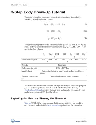
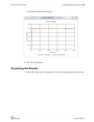
1. STAR-CCM+ User Guide
4410
Combustion
Tutorials
Three types of models have been chosen for combustion tutorials:
• An idealized CAN type gas turbine combustion chamber
• A flame tube
• Methane on platinum
These models will familiarize you with STAR-CCM+’s combustion
modeling capabilities and introduce various recommended practices for
simulating combusting flows.
CAN Type Gas Turbine Combustion Chamber
The problem geometry (shown below) consists of three sets of air inlets
placed circumferentially at the combustor head to promote maximum
mixing and flame stabilization. Swirling air enters the primary combustion
zone through the two sets of inlets nearest to the axis of symmetry.
Non-swirling air enters the upper inlet and thence the primary, secondary
and dilution zones via five injection holes in the baffle.
Air is assumed to be composed of 23.3% oxygen and 76.7% nitrogen, by
mass, and its initial pressure and temperature are 1 bar and 293 K,
respectively.
Version 4.04.011

2. STAR-CCM+ User Guide
4411
The use of periodic interfaces allows the cylindrical combustor to be
represented by a single sixty-degree sector, reducing the computational
effort required by a factor of roughly 5 ⁄ 6 .
The combustion models illustrated using the above geometry are:
• Propane combustion using a 3-step Eddy Break-up model.
• Propane combustion using an adiabatic PPDF model.
• Hydrogen combustion using an adiabatic PPDF Flamelets model.
Flame Tube
The problem geometry consists of a two-dimensional representation of a
flame tube. The flow involves an inviscid, compressible, multi-component
gas whose components are reacting chemically. A premixed mixture of
hydrogen and air enters the pipe through an inlet at a pressure of 1 bar and
a temperature of 1000K.
The combustion model illustrated using this geometry is the complex
chemistry operator splitting model.
Methane on Platinum
Methane on platinum deposition is modeled by importing complex
chemistry descriptions from external files. In this simulation, a premixed
combination of methane and air flows over a platinum plate at a pressure of
1 bar and a temperature of 600K.
Version 4.04.011

3. STAR-CCM+ User Guide
4412
3-Step Eddy Break-Up Tutorial
This tutorial models propane combustion in air using a 3-step Eddy
Break-up model as detailed below:
C 3 H 8 + 1.5O 2 → 3CO + 4H 2
(9)
CO + 0.5O 2 → CO 2
(10)
H 2 + 0.5O 2 → H 2 O
(11)
The physical properties of the air components (23.3% O2 and 76.7% N2, by
mass) and the rest of the reaction components (C3H8 , CO, H2 , CO2 , H2O)
are defined as follows:
O2
N2
C3H
CO
H2
8
Molecular weights
Density
Molecular viscosity
Specific heat
Thermal conductivity
32.0
28.00
8
CO
O
2
44.1
28.0
1
2.01
44.01
H2
18.02
8
Ideal gas
1.716 x 10–5 Pas
Determined via thermodynamic polynomial functions
Determined via the Lewis number
Air enters the combustion chamber through the three air inlets and propane
gas enters through the fuel inlet, as indicated in the introductory
Combustion Tutorials section. Both air and fuel are at a pressure of 1 bar
and a temperature of 293 K at the inlets.
Importing the Mesh and Naming the Simulation
Start up STAR-CCM+ in a manner that is appropriate to your working
environment and select the New Simulation option from the menu bar.
Version 4.04.011

4. STAR-CCM+ User Guide
3-Step Eddy Break-Up Tutorial 4414
Visualizing the Imported Geometry
To view the geometry more clearly, change the viewing direction.
• Open the Scenes > Geometry Scene 1 > Attributes node, then right-click
on the View node.
• Select Edit....
• In the Edit View dialog, enter the values shown below and then click
Apply.
• Close the Edit View dialog.
To make the interior features of the combustor geometry visible, change the
opacity of its surfaces.
Version 4.04.011

5. STAR-CCM+ User Guide
3-Step Eddy Break-Up Tutorial 4420
• First select the Segregated Flow node.
• In the Properties window, change the Convection property to 1st-order.
• Repeat this process for the Segregated Species, Segregated Fluid Enthalpy
and Standard K-Epsilon nodes.
• Save the simulation by clicking on the
(Save) button.
Setting Material Properties
The components of the mixture and its material properties must now be
defined.
Version 4.04.011

6. STAR-CCM+ User Guide
3-Step Eddy Break-Up Tutorial 4424
• Select the C3H8 > Component Properties > Specific Heat node.
• In the Properties window, change the Method property to Thermodynamic
Polynomial Data
• Repeat this process for the remaining six components.
This completes the specification of material properties.
• Save the simulation.
Defining Reactions
• Within the Models node, select the Eddy Break-up node.
Version 4.04.011

7. STAR-CCM+ User Guide
3-Step Eddy Break-Up Tutorial 4427
• Select the C3H8 node and, in the Properties window, enter 1.0 for the
Stoich. Coeff.
• Repeat this for O2 , CO and H2 , assigning stoichiometric coefficients of
1.5, 3.0 and 4.0, respectively.
The specification of Reaction 1 is now complete.
• Follow the same procedure to define the remaining two reactions of the
chemical reaction scheme:
CO + 0.5O 2 → CO 2
(12)
H 2 + 0.5O 2 → H 2 O
(13)
• Save the simulation.
Setting Initial Conditions and Reference Values
The lower temperature limit for the specific heat polynomials imported
from the materials database is 200 K. Although this temperature is much
lower than we would expect to find in the converged solution, it is possible
that temperatures below this may arise early on in the run. For this reason,
it is necessary to increase the minimum allowable temperature to match the
lower temperature limit for the polynomials.
Version 4.04.011

8. STAR-CCM+ User Guide
3-Step Eddy Break-Up Tutorial 4430
• In the Properties window, set the Value property to 293 K.
• Select the Turbulence Specification node.
• In the Properties window, select Intensity + Length Scale for the Method
property.
• Set the turbulence intensity to 0.05 and the turbulent length scale to
0.2.
• Save the simulation.
Creating Interfaces
All regions and boundaries already have suitable names so we can proceed
to create the periodic interface linking the two plane, rectangular, cyclic
boundaries.
• Open the Regions > Default_Fluid > Boundaries node.
A node will be displayed for each boundary region.
Version 4.04.011

9. STAR-CCM+ User Guide
3-Step Eddy Break-Up Tutorial 4432
Two new periodic boundary nodes will appear under the Boundaries node
and a new node named Periodic 1 will appear under the Interfaces node.
Setting Boundary Conditions and Values
All wall boundaries, including the baffle, are adiabatic, no-slip walls. Since
this is the default wall boundary type, no changes are required here. The
default settings are also suitable for the outlet, so the only boundary
conditions that need to be specified are for the four inlets.
• Select the Air_Inlet1 > Physics Conditions > Velocity Specification node.
• In the Properties window, change the Method property to Components.
• Select the Turbulence Specification node and, in the Properties window,
change the Method property to Intensity + Length Scale.
The air and fuel will be made to swirl on entry to the combustor by
specifying inlet velocity vectors in a new cylindrical coordinate system. To
create the latter:
• Open the Tools node, right-click the Coordinate Systems node and then
Version 4.04.011

10. STAR-CCM+ User Guide
3-Step Eddy Break-Up Tutorial 4440
• Click OK.
• Select the Fuel_Inlet > Physics Values > Velocity > Constant node.
• In the Properties window enter -28,-60,100 m/s for the Value property.
Specification of the boundary conditions is now complete.
• Save the simulation.
Setting Solver Parameters and Stopping Criteria
The default under-relaxation factors for the flow and turbulence equations
are suitable for this case but those for the species and energy equations need
to be reduced to ensure solution convergence.
• Select the Solvers > Segregated Species node.
• In the Properties window, change the Under-Relaxation Factor property to
0.8
• Select the Segregated Energy node and change the Fluid Under-Relaxation
Factor property to 0.8 also.
It is important that the under-relaxation factors for the species and energy
equations are the same to ensure that the two solutions remain
synchronized. Other species and energy modeling settings, such as the
choice of differencing scheme, should also be kept the same.
The simulation will be run for 500 iterations, which is sufficient to achieve a
steady-state solution. This number can be specified using a stopping
criterion.
Version 4.04.011

11. STAR-CCM+ User Guide
3-Step Eddy Break-Up Tutorial 4447
• Add the plane section part to the Selected list.
• Click Close.
• Right-click on the scalar bar in the display. In the pop-up menu that
appears, select Temperature.
• Rotate the scalar scene until the view is roughly perpendicular to the
plane section (which is colored beige in the geometry scene), and the
inlet boundaries are on the left.
• Save the simulation.
Reporting, Monitoring and Plotting
STAR-CCM+ can dynamically monitor virtually any quantity while the
solution develops. This requires setting up a report defining the quantity of
interest and the parts of the region to be monitored. A monitor is then
defined based on that report. The former also helps to create an appropriate
X-Y graph plot.
Version 4.04.011

12. STAR-CCM+ User Guide
3-Step Eddy Break-Up Tutorial 4452
• Rename the Carbon In Plot node as Carbon Balance.
• Make sure that the Title property of the Carbon Balance node is Carbon
Balance.
• Double-click the Carbon Balance node to display the empty plot in the
Graphics window.
The analysis is now ready to be run.
• Save the simulation.
Running the Simulation
• To run the simulation, click the
(Run) button on the toolbar.
If this is not displayed, use the Solution > Run menu item. You may also
activate the Solution toolbar by selecting Tools > Toolbars > Solution and then
clicking the toolbar button.
The Residuals display will be created automatically and will show the
solver’s progress. If necessary, click on the Residuals tab to bring the
Residuals plot into view. An example of a residual plot is shown in a
separate part of the User Guide. This example will look different from your
residuals, since the plot depends on the models selected.
Version 4.04.011

13. STAR-CCM+ User Guide
3-Step Eddy Break-Up Tutorial 4454
solution has indeed converged.
• Save the simulation.
Visualizing the Results
• Select the Scalar Scene 1 display to view the temperature profile for the
Version 4.04.011

14. STAR-CCM+ User Guide
3-Step Eddy Break-Up Tutorial 4457
angle so that velocity vectors are clearly visible.
Summary
This tutorial introduced the following STAR-CCM+ features:
• Importing the mesh and saving the simulation.
• Visualizing the geometry.
• Defining models for eddy break-up combustion.
• Defining material properties required for multi-component gases.
• Defining chemical reactions.
• Setting initial conditions and reference values.
• Creating interfaces.
• Defining boundary conditions.
• Setting solver parameters and stopping criteria.
• Creating vector and scalar displays for examining the results.
• Setting up monitoring reports and plots.
• Running the solver for a set number of iterations.
• Analyzing the results using STAR-CCM+’s visualization facilities.
Version 4.04.011

15. STAR-CCM+ User Guide
Adiabatic PPDF Equilibrium Tutorial 4459
combustor.ccm.
• Click Open to start the import. The Import Mesh Options dialog will
appear. Select the following options:
•
Run mesh diagnostics after import
•
Open geometry scene after import
• Ensure that the Don’t show this dialog during import option is not selected
and then click OK.
STAR-CCM+ will provide feedback on the import process, which will take
a few seconds, in the Output window. A geometry scene showing the
combustor geometry will be created in the Graphics window.
• Finally, save the new simulation to disk under file name
adiabaticPPDF.sim.
Visualizing the Imported Geometry
To view the geometry more clearly, change the viewing direction.
• Right-click the Scenes > Geometry Scene 1 > Attributes > View node and
Version 4.04.011

16. STAR-CCM+ User Guide
Adiabatic PPDF Equilibrium Tutorial 4461
• Open the Displayers node and select the Geometry 1 node.
• In the Properties window, change the Opacity property to 0.2.
The baffle and the five injection holes in it are now visible through the
external surface of the combustor.
You can now proceed to Setting up the Models.
Setting up the Models
Models define the primary variables of the simulation, including pressure,
temperature and velocity, and what mathematical formulation will be used
to generate the solution. In this example, the flow involves a turbulent,
compressible, multi-component gas whose components are reacting
chemically. The Segregated Flow model will be used together with the
standard K-Epsilon turbulence model and the PPDF reaction model.
To select the models:
• Open the Continua node, right-click on the Physics 1 node and select
Version 4.04.011

17. STAR-CCM+ User Guide
Adiabatic PPDF Equilibrium Tutorial 4466
node.
• In the Properties window, change the Convection property to 1st-order.
• Repeat this process for the Adiabatic PPDF and Standard K-Epsilon nodes.
• Save the simulation by clicking the
(Save) button.
The next step is Defining Mixture Components.
Defining Mixture Components
The PPDF table used in this tutorial involves only six gaseous species: C3H8,
O2, N2, CO, CO2 and H2O which, for demonstration purposes, should
provide a solution of reasonable accuracy. A more realistic solution could
be obtained by including additional intermediate species in the table.
To define the gas components corresponding to the above species:
Version 4.04.011

18. STAR-CCM+ User Guide
Adiabatic PPDF Equilibrium Tutorial 4468
do not need to be changed so we can now proceed to Generating the PPDF
Table.
Generating the PPDF Table
First, we will change the number of heat loss ratio points defined in the
table:
• Select the PPDF Equilibrium Table node.
• In the Properties window, make sure that the Number of heat loss ratio
points equals 1.
• Change the Relative Pressure of the mixture property to 0.0 Pa.
Now define the fuel and oxidizer streams:
• Select the Fluid Stream Manager > Fuel Stream node.
Change the Temperature of the stream property to 293 K.
• Right-click on the Fuel Stream > Components node and select
Version 4.04.011

19. STAR-CCM+ User Guide
Adiabatic PPDF Equilibrium Tutorial 4471
Setting Initial Conditions
The combustor’s initial condition is a stationary flow field consisting
entirely of air. The default values of initial mixture fraction, mixture fraction
variance and velocity are all zero so no changes to the initial conditions are
required.
Creating Interfaces
All regions and boundaries already have suitable names so we may now
create the periodic interface linking the two plane, rectangular, cyclic
boundaries.
• Open the Regions > Default_Fluid > Boundaries node.
A node is shown for each boundary region.
• Ctrl+click to select the Cyclic1 and Cyclic2 nodes.
Version 4.04.011

20. STAR-CCM+ User Guide
Adiabatic PPDF Equilibrium Tutorial 4479
• In the Properties window, enter a Value of 1.0.
• Select the Fuel_Inlet > Physics Values > Velocity > Constant node.
• In the Properties window enter -28,-60,100 m/s for the Value property.
Specification of the boundary conditions is now complete.
• Save the simulation.
Setting Stopping Criteria
Adjust the maximum number of iterations so that the calculation will run
for 600 iterations, which should be sufficient for a steady-state solution. This
number can be specified using a stopping criterion.
• Open the Stopping Criteria node and then select the Maximum Steps node.
• Change the Maximum Steps property to 600.
The solution will not run beyond 600 iterations, unless this stopping
criterion is changed or disabled.
• Save the simulation.
Version 4.04.011

21. STAR-CCM+ User Guide
Adiabatic PPDF Equilibrium Tutorial 4482
appears, select Temperature.
• Select the Scenes > Geometry Scene 1 > Displayers > Section Scalar 1
node.
• In the Properties window, change the Contour Style property to Smooth
Filled.
• Rotate the geometry scene until the view is roughly perpendicular to
the beige plane section and the inlet boundaries are on the left.
• Save the simulation.
Running the Simulation
• To run the simulation, click the
(Run) button on the toolbar.
Version 4.04.011

22. STAR-CCM+ User Guide
Adiabatic PPDF Equilibrium Tutorial 4484
Visualizing the Results
• Go to the Geometry Scene 1 display to view the temperature profile for
the converged solution.
• Right-click on the scalar bar in the Geometry Scene 1 display and select
Version 4.04.011

23. STAR-CCM+ User Guide
Adiabatic PPDF Equilibrium Tutorial 4488
The resulting scene is shown below.
It will be seen that the ratio’s value is generally rather high, implying that
the predicted maximum temperature is considerably lower than the
adiabatic flame temperature. In a realistic modeling exercise, a considerably
finer mesh would be needed to increase confidence in the calculated
temperatures.
Summary
This tutorial introduced the following STAR-CCM+ features:
• Importing the mesh and saving the simulation.
• Visualizing the geometry.
• Defining an adiabatic PPDF combustion model.
• Generating a PPDF table.
• Creating interfaces.
• Defining boundary conditions.
• Setting stopping criteria.
• Creating scalar displays for examining the results.
Version 4.04.011

24. STAR-CCM+ User Guide
4490
Adiabatic PPDF Flamelets Tutorial
In this tutorial, a hydrogen combustion case is set up using the PPDF
Laminar Flamelets reaction model for unpremixed flames. The model
assumes adiabatic conditions (no heat loss) and accounts for
non-equilibrium and finite-rate chemistry effects.
For adiabatic PPDF, the physical properties of the fuel (hydrogen in this
case) are not utilized directly by STAR-CCM+ as no additional transport
equations requiring these properties are solved. Temperature, density and
species mass fractions are evaluated using the β function formulation (see
the Adiabatic Equilibrium Model section in the User Guide).
Air enters the combustion chamber through the three air inlets and
hydrogen gas enters through the fuel inlet, as indicated in the introductory
Combustion Tutorials section.
Importing the Mesh and Naming the Simulation
Start up STAR-CCM+ in a manner that is appropriate to your working
environment and select the New Simulation option from the menu bar.
Continue by importing the mesh and naming the simulation. A
predominantly hexahedral cell mesh has been prepared for this analysis.
and saved in the STAR .ccm file format.
• Select File > Import... from the menu bar.
• In the Open dialog, simply navigate to the doc/tutorials/combustor
subdirectory of your STAR-CCM+ installation directory and select file
Version 4.04.011

25. STAR-CCM+ User Guide
Adiabatic PPDF Flamelets Tutorial 4493
• Open the Displayers node and select the Geometry 1 node.
• In the Properties window, change the Opacity expert property to 0.2.
The baffle and the five injection holes in it are now visible through the
external surface of the combustor.
You can now proceed to Setting up the Models
Setting up the Models
Models define the primary variables of the simulation, including pressure,
temperature and velocity, and what mathematical formulation will be used
to generate the solution. In this example, the flow involves a turbulent,
compressible, multi-component gas whose components are reacting
chemically. The Segregated Flow model will be used together with the
standard K-Epsilon turbulence model and the PPDF reaction model.
To select the models:
• Open the Continua node, right-click on the Physics 1 node and select
Version 4.04.011