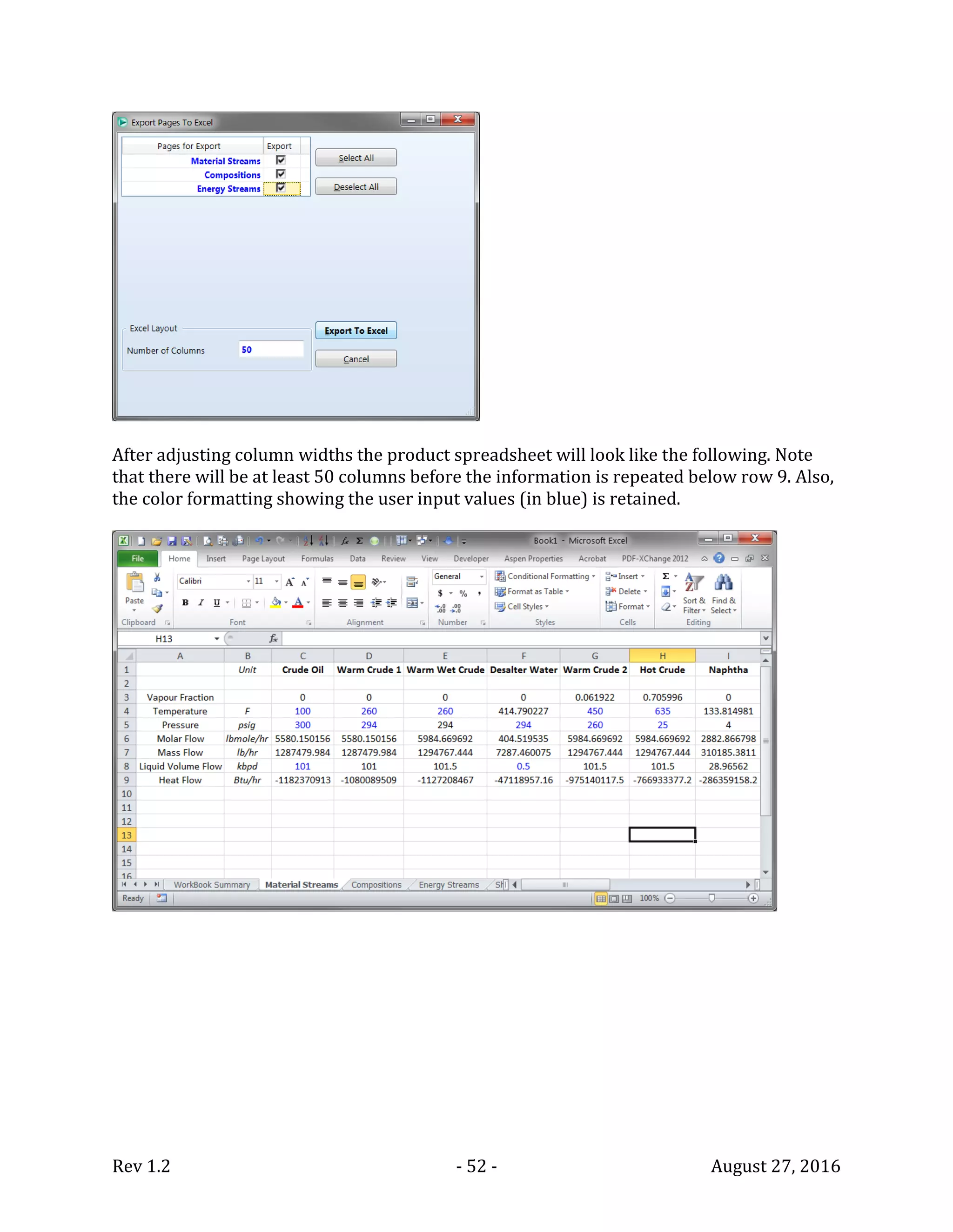
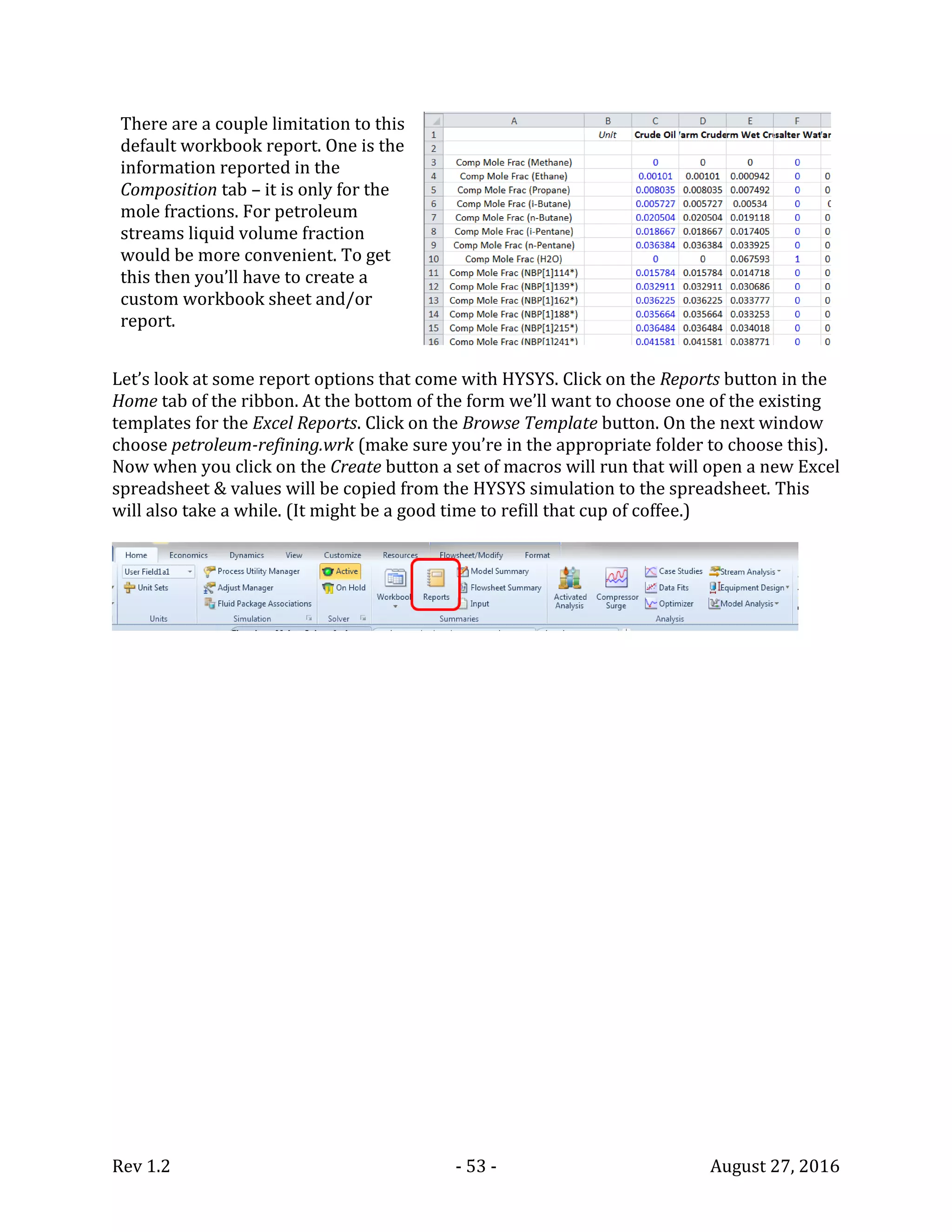
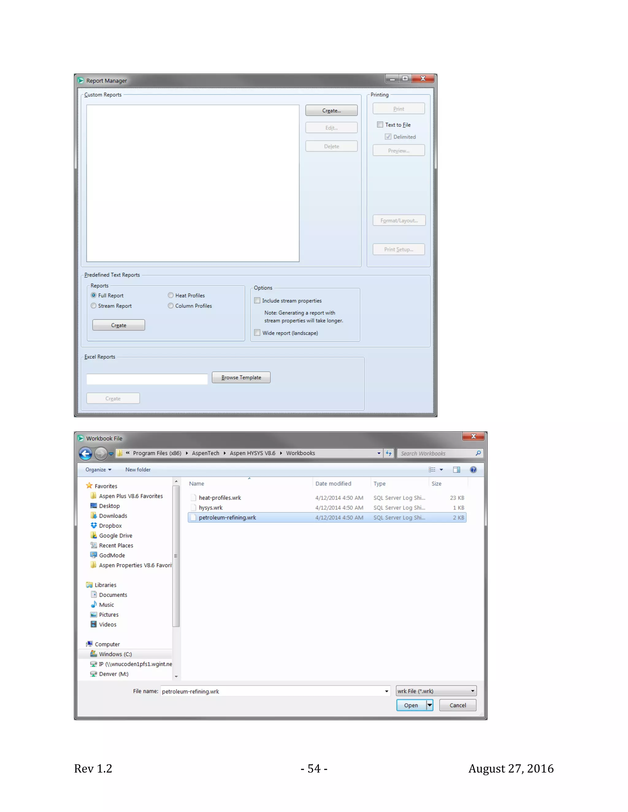
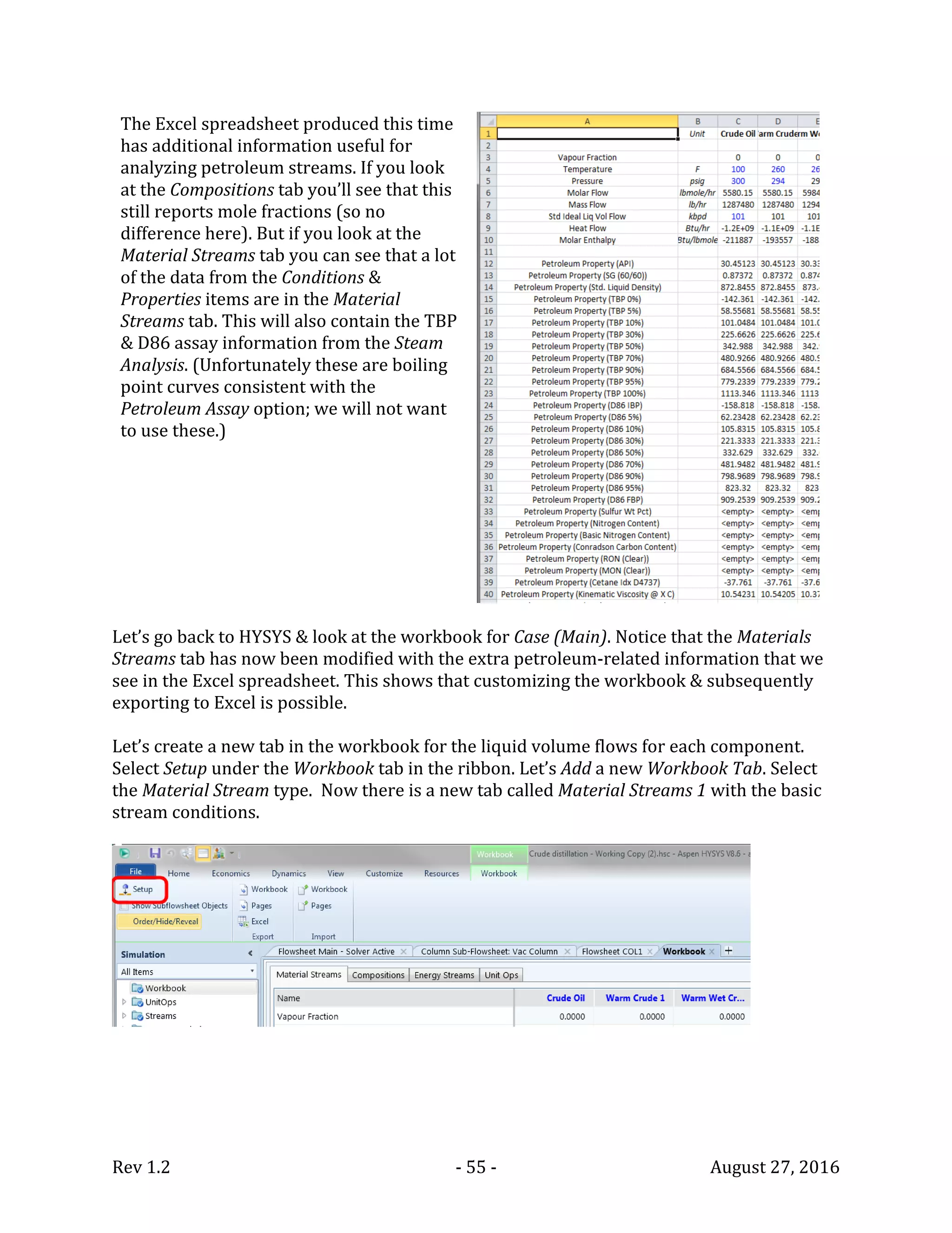
Download to read offline
![Rev 1.2 - 3 - August 27, 2016
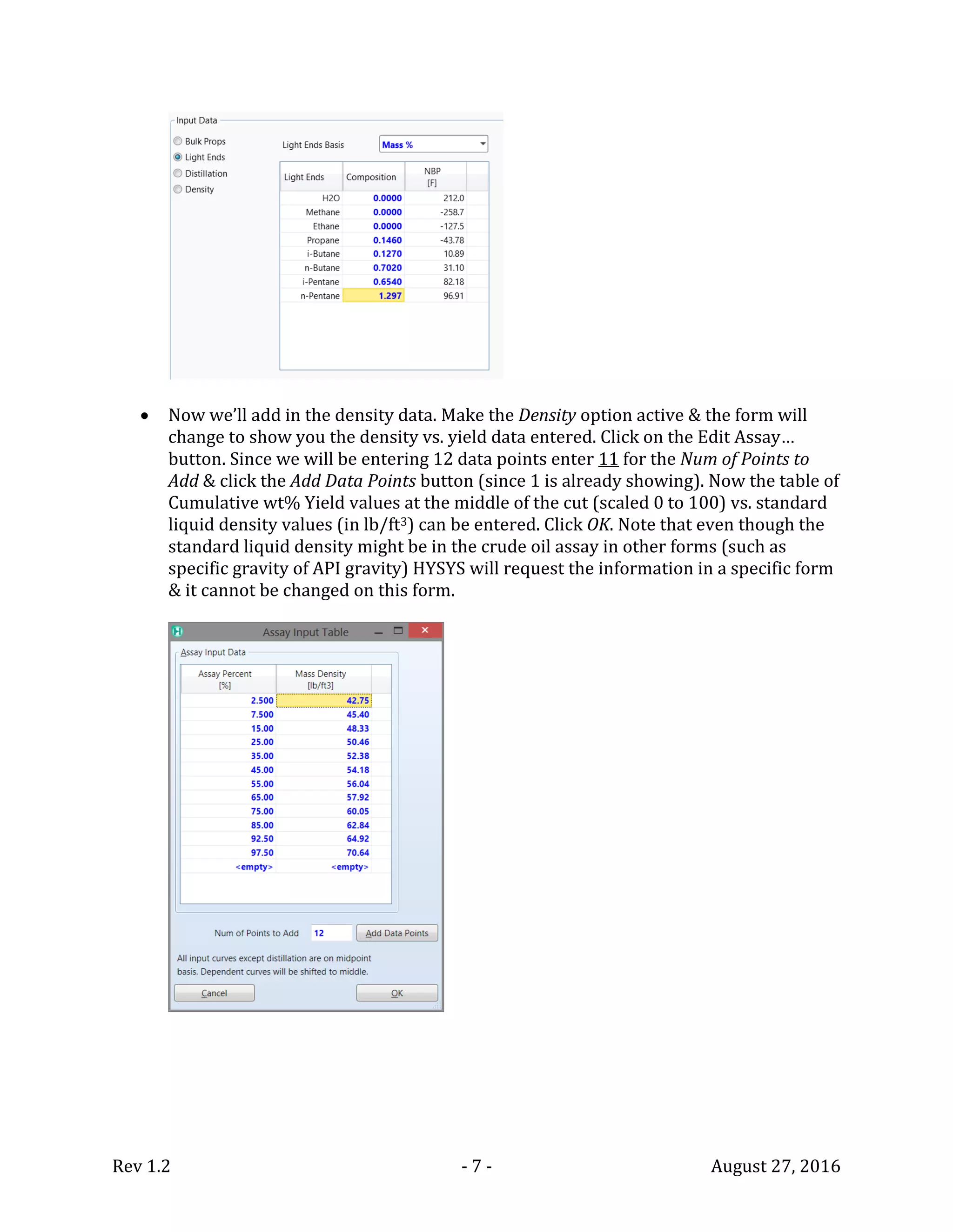
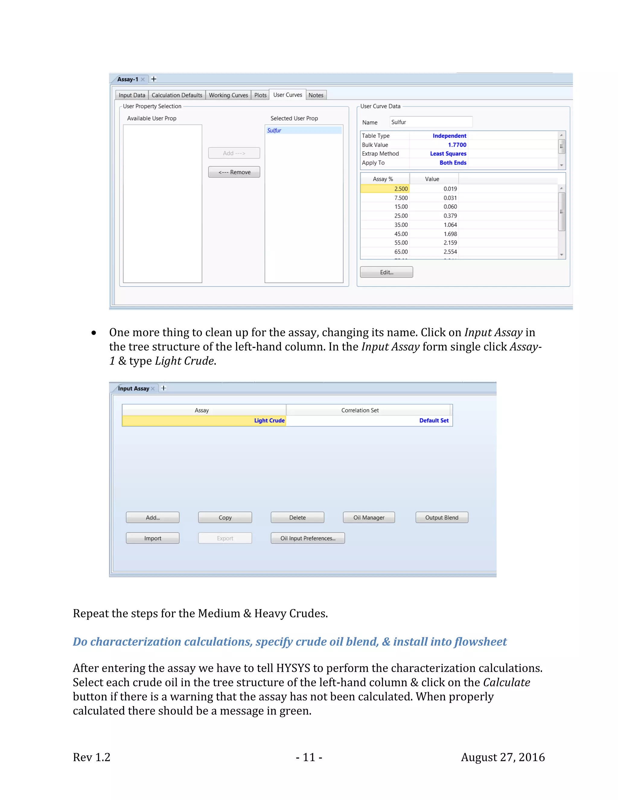
We now want to add assay data for the three crude oils: Light Crude, Medium Crude, &
Heavy Crude. The data to be added is shown in the following tables.
Table 1. Assay Data for Light Crude
Light Crude
Cumulative Yield
[wt%] Density Sulfur Light Ends Analysis
IBP EP @ IBP @ Mid lb/ft31
wt% [wt%]
Whole Crude 53.27 1.77 Ethane 0.000
31 160 0 2.5 42.75 0.019 Propane 0.146
160 236 5 7.5 45.40 0.031 i-Butane 0.127
236 347 10 15 48.33 0.060 n-Butane 0.702
347 446 20 25 50.46 0.379 i-Pentane 0.654
446 545 30 35 52.38 1.064 n-Pentane 1.297
545 649 40 45 54.18 1.698
649 758 50 55 56.04 2.159
758 876 60 65 57.92 2.554
876 1015 70 75 60.05 3.041
1015 1205 80 85 62.84 3.838
1205 1350 90 92.5 64.92 4.503
1350 FBP 95 97.5 70.64 6.382
1 Note that HYSYS uses a water density to convert to specific gravity of 62.3024 lb/ft³ =8.32862 lb/gal =
997.989 kg/m³.](https://image.slidesharecdn.com/crudetowersimulation-hysysv8-190925050009/75/Crude-tower-simulation-hysys_v8-6-3-2048.jpg)
![Rev 1.2 - 4 - August 27, 2016
Table 2. Assay Data for Medium Crude
Medium Crude
Cumulative Yield
[wt%] Density Sulfur Light Ends Analysis
IBP EP @ IBP @ Mid lb/ft3 wt% [wt%]
Whole Crude 55.00 2.83 Ethane 0.000
88 180 0 2.5 43.47 0.022 Propane 0.030
180 267 5 7.5 47.14 0.062 i-Butane 0.089
267 395 10 15 49.42 0.297 n-Butane 0.216
395 504 20 25 51.83 1.010 i-Pentane 0.403
504 611 30 35 54.08 2.084 n-Pentane 0.876
611 721 40 45 55.90 2.777
721 840 50 55 57.73 3.284
840 974 60 65 59.77 3.857
974 1131 70 75 62.30 4.706
1131 1328 80 85 65.74 5.967
1328 1461 90 92.5 68.08 6.865
1461 FBP 95 97.5 73.28 8.859
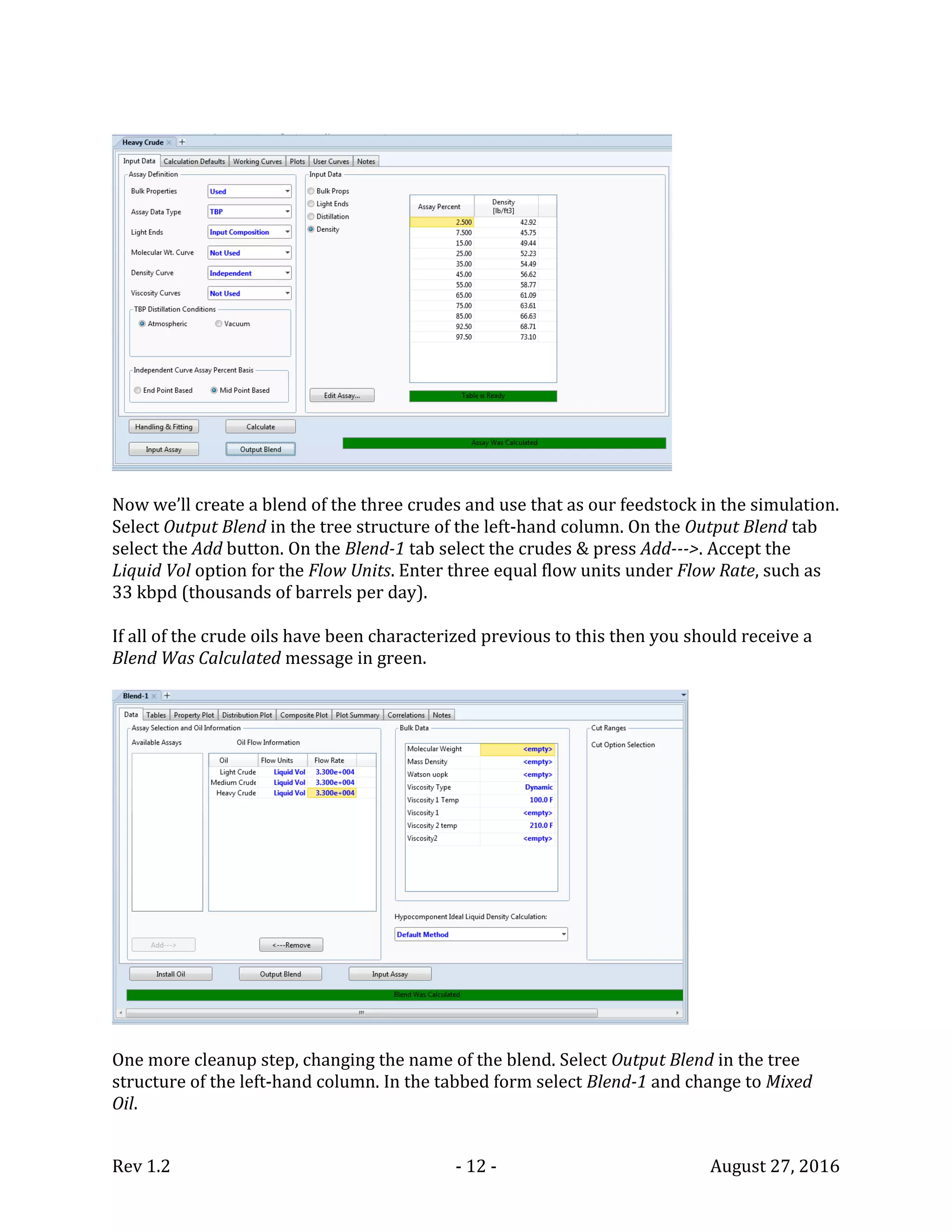
Table 3. Assay Data for Heavy Crude
Heavy Crude
Cumulative Yield
[wt%] Density Sulfur Light Ends Analysis
IBP EP @ IBP @ Mid lb/ft3 wt% [wt%]
Whole Crude 55.20 2.8 Ethane 0.039
27 154 0 2.5 42.92 0.005 Propane 0.284
154 255 5 7.5 45.75 0.041 i-Butane 0.216
255 400 10 15 49.44 0.341 n-Butane 0.637
400 523 20 25 52.23 1.076 i-Pentane 0.696
523 645 30 35 54.49 1.898 n-Pentane 1.245
645 770 40 45 56.62 2.557
770 902 50 55 58.77 3.185
902 1044 60 65 61.09 3.916
1044 1198 70 75 63.61 4.826
1198 1381 80 85 66.63 5.990
1381 1500 90 92.5 68.71 6.775
1500 FBP 95 97.5 73.10 8.432](https://image.slidesharecdn.com/crudetowersimulation-hysysv8-190925050009/75/Crude-tower-simulation-hysys_v8-6-4-2048.jpg)
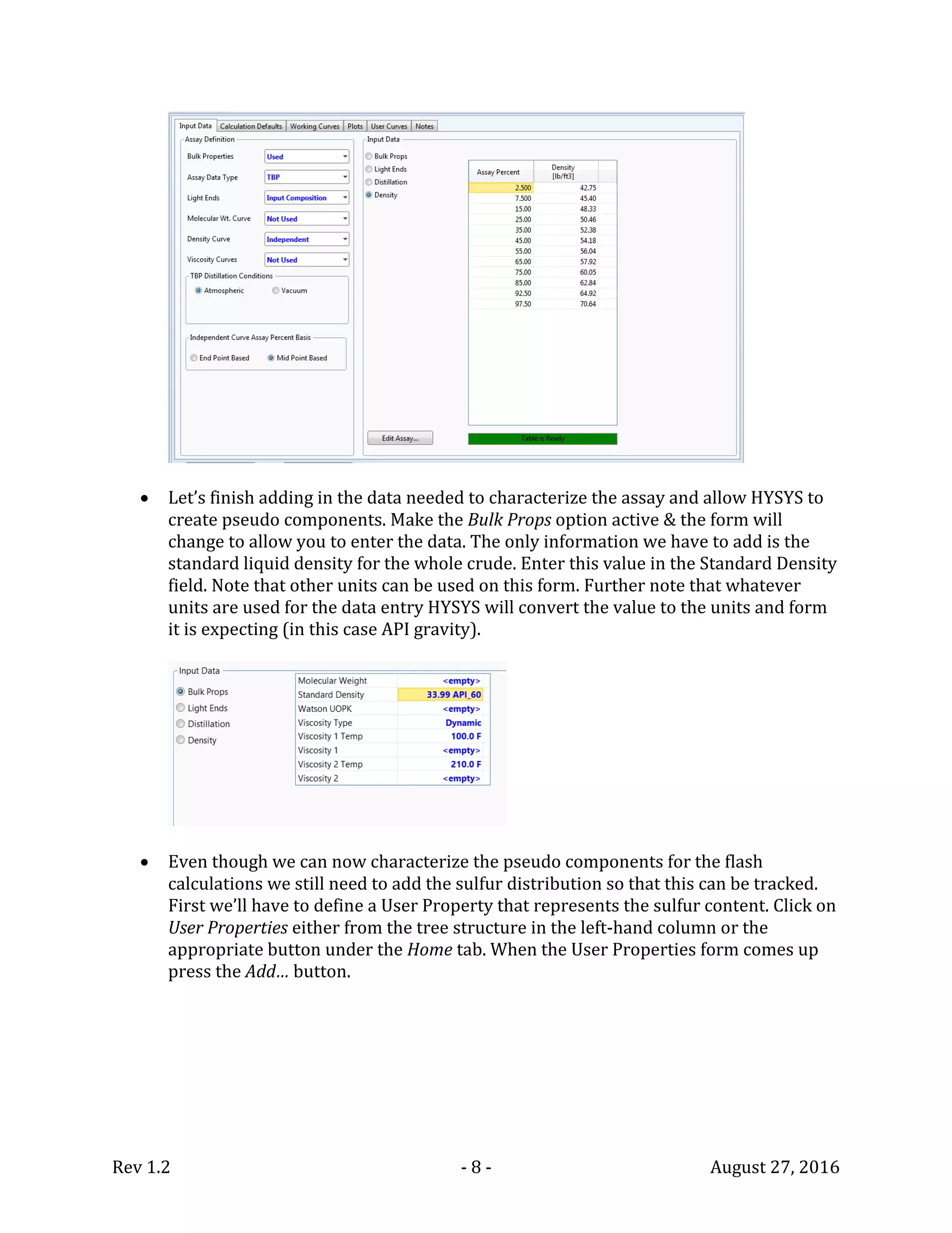
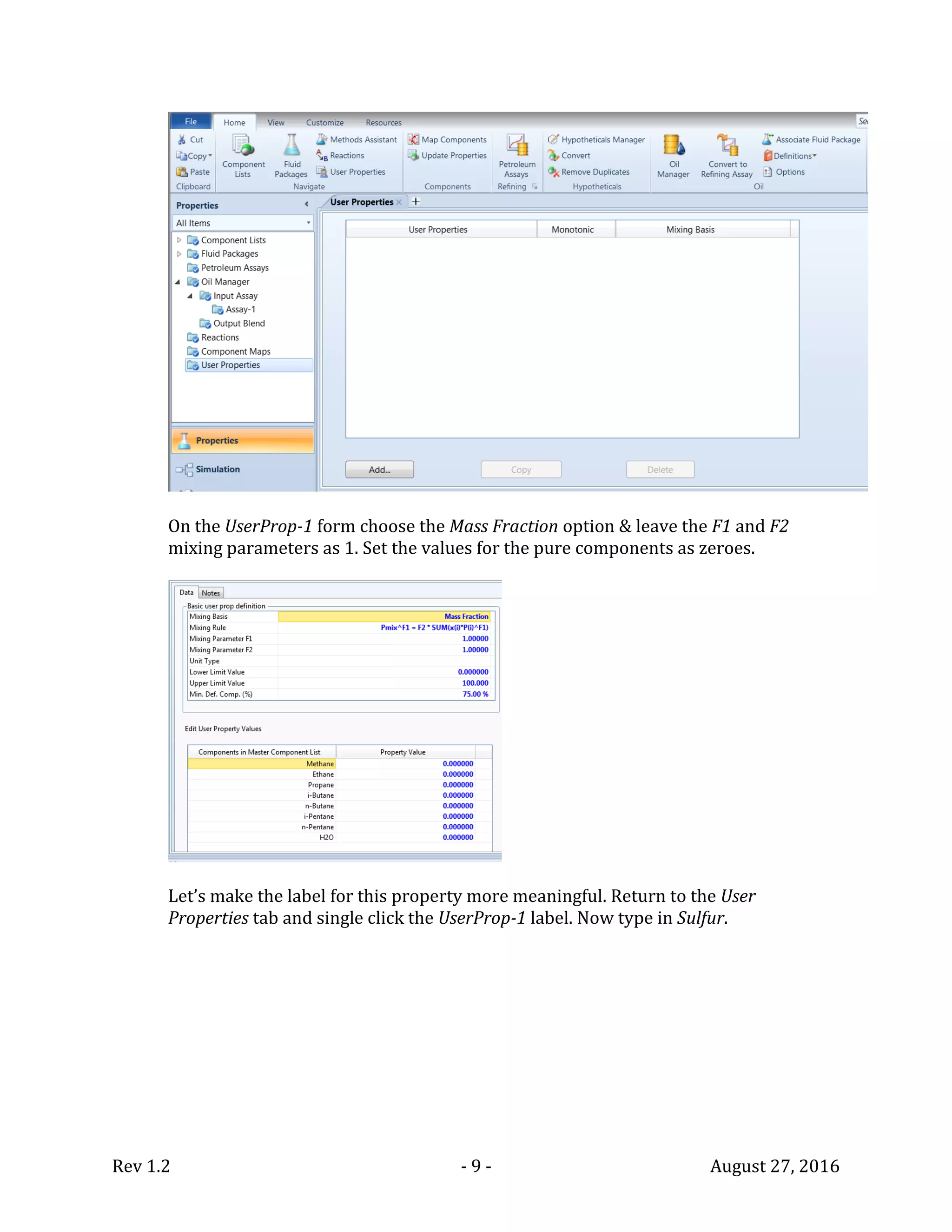
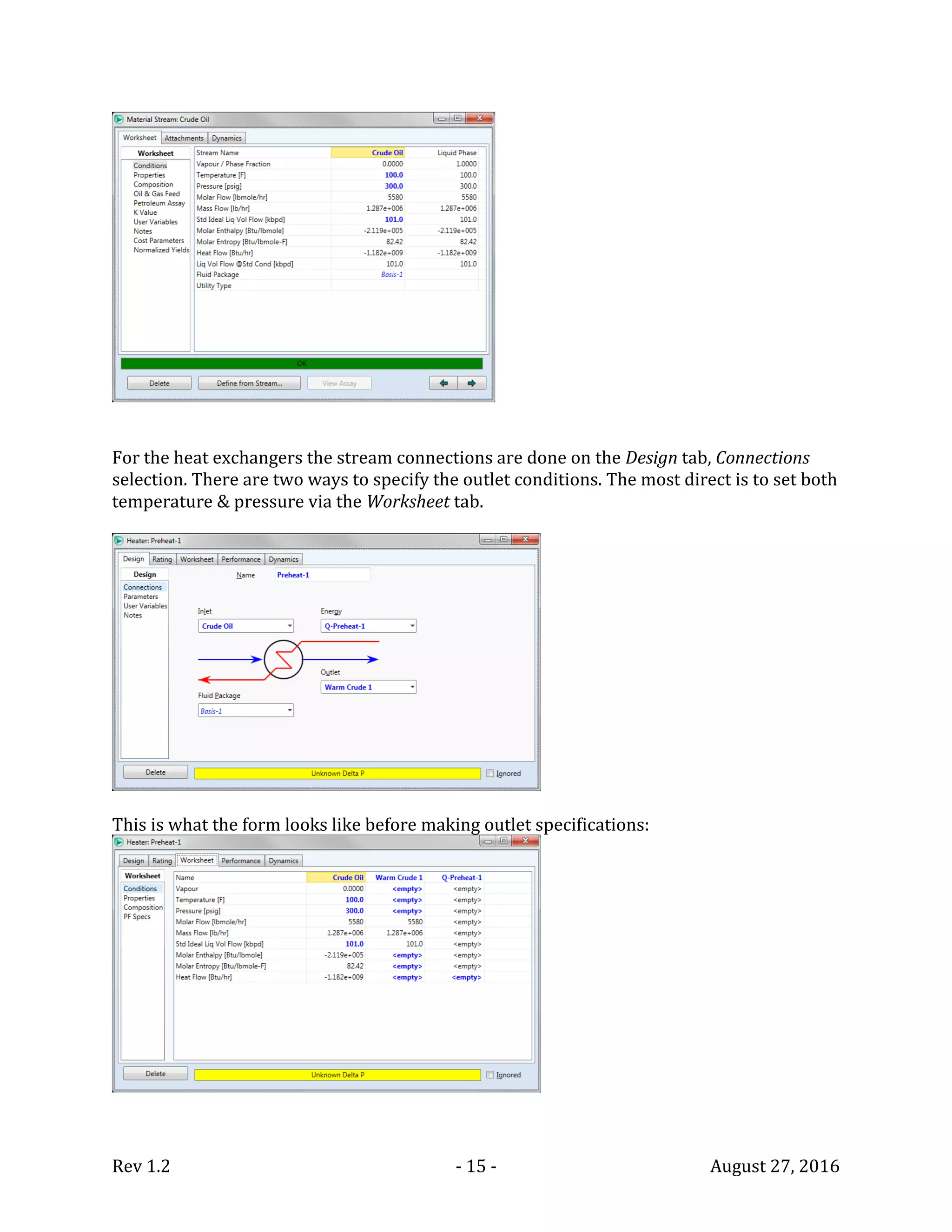
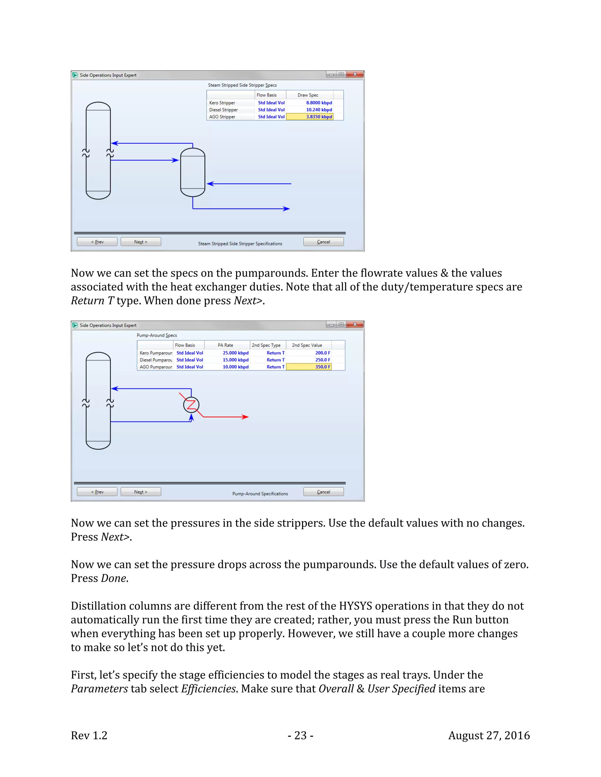

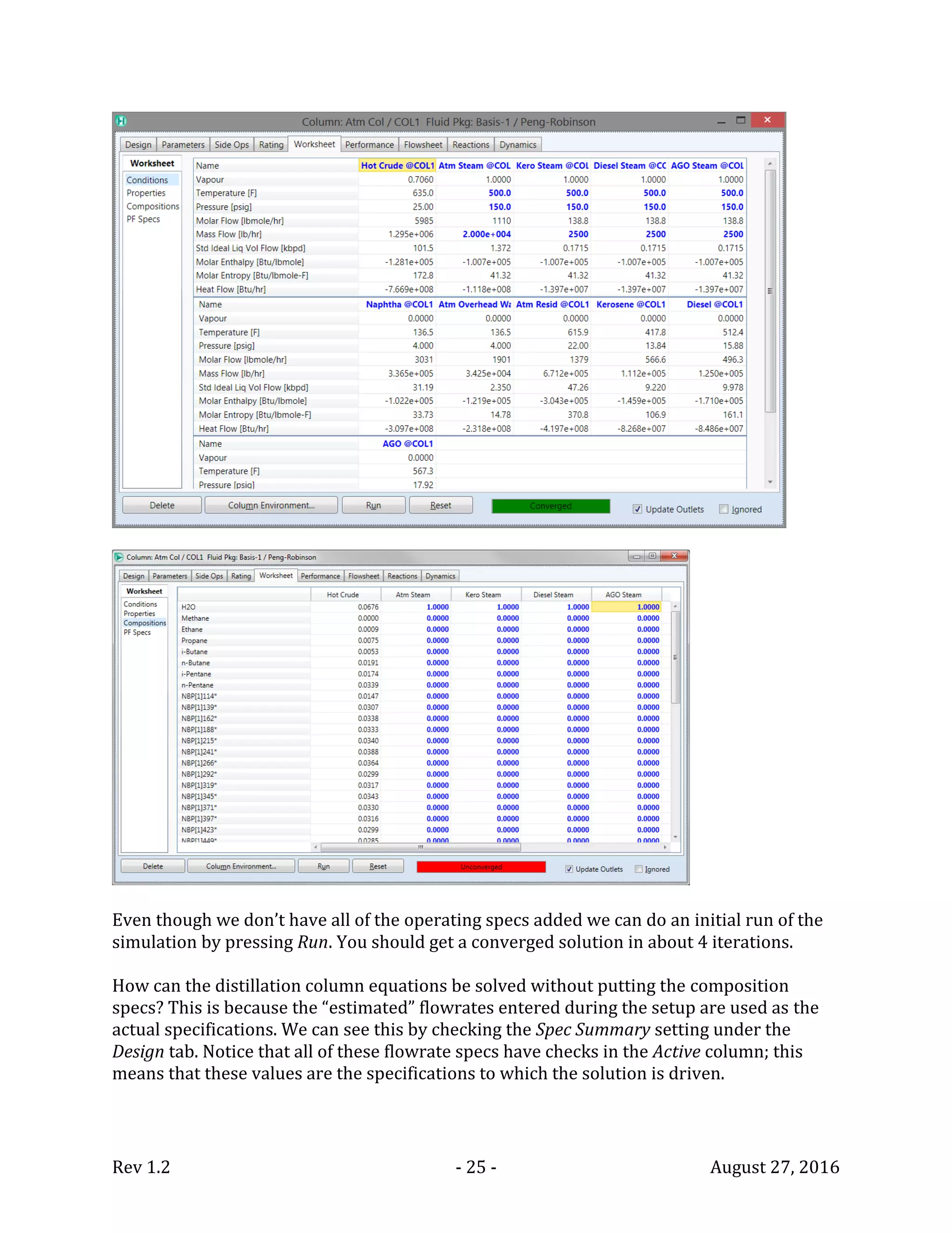
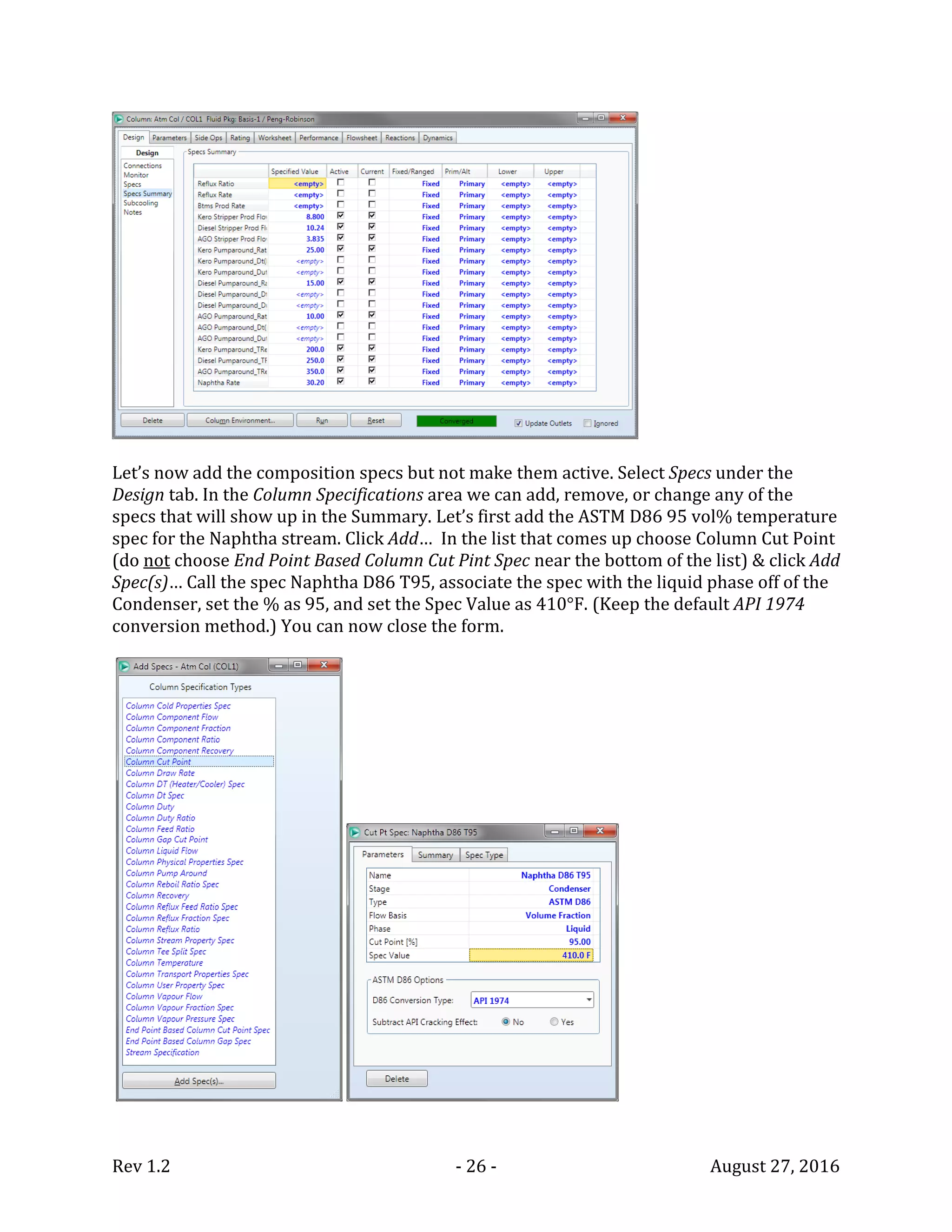
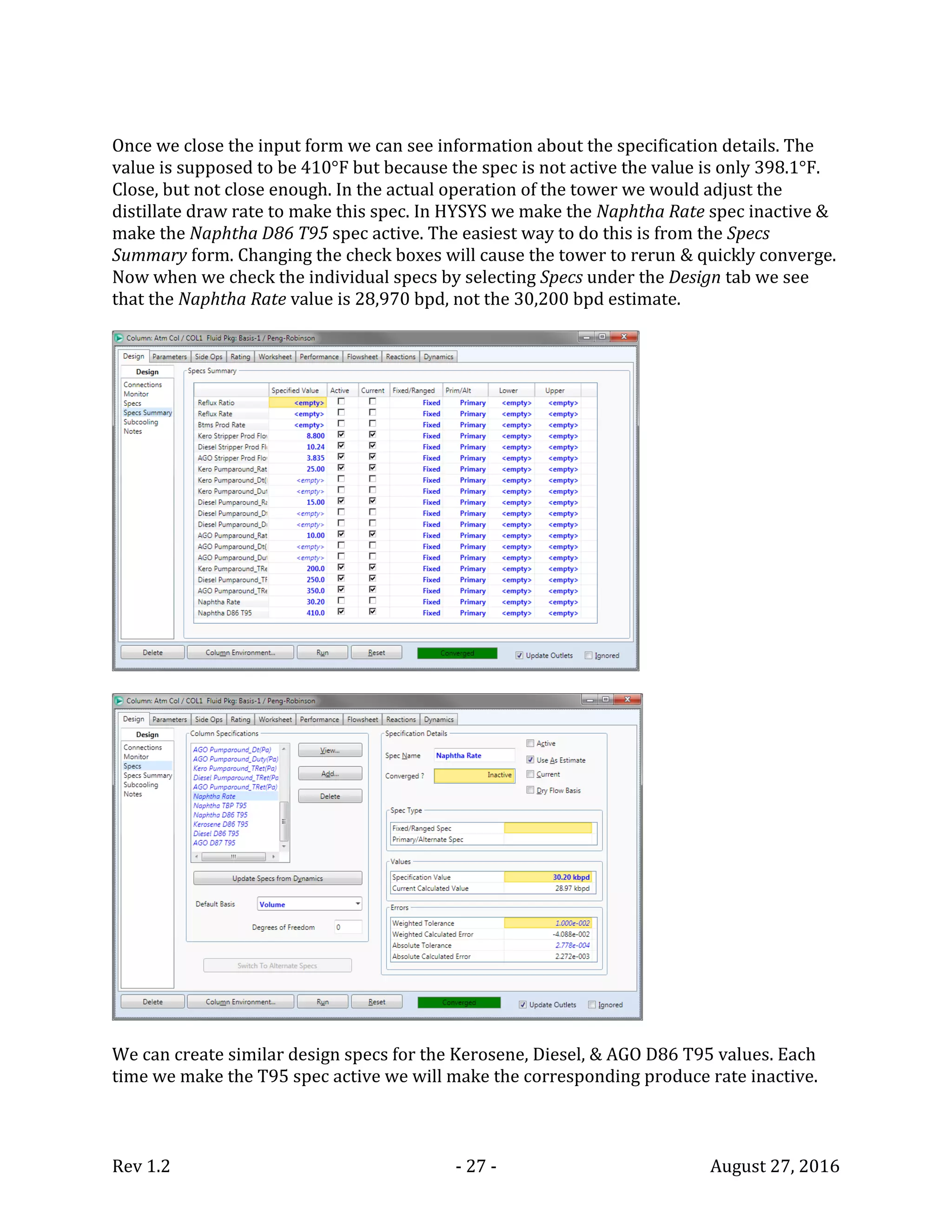
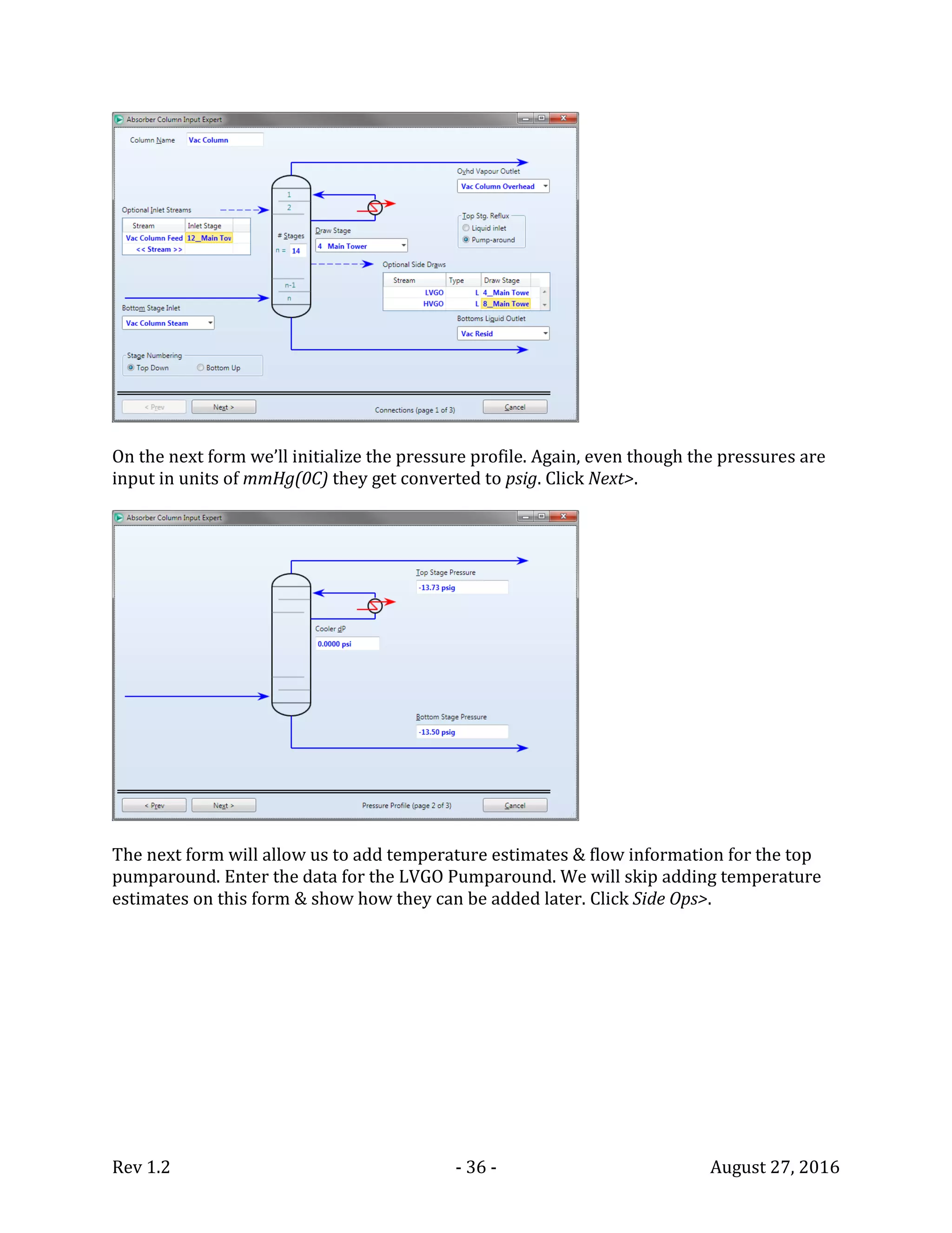
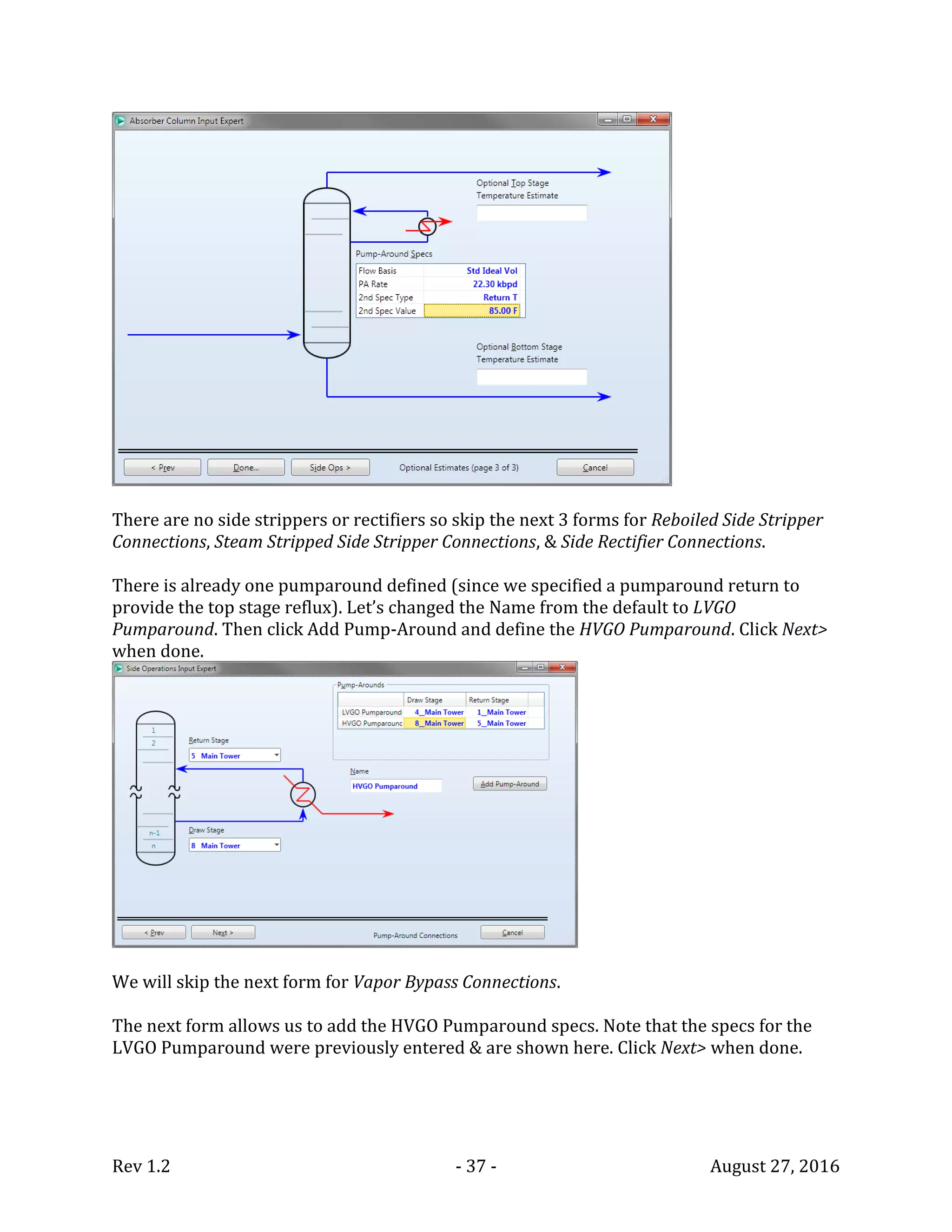
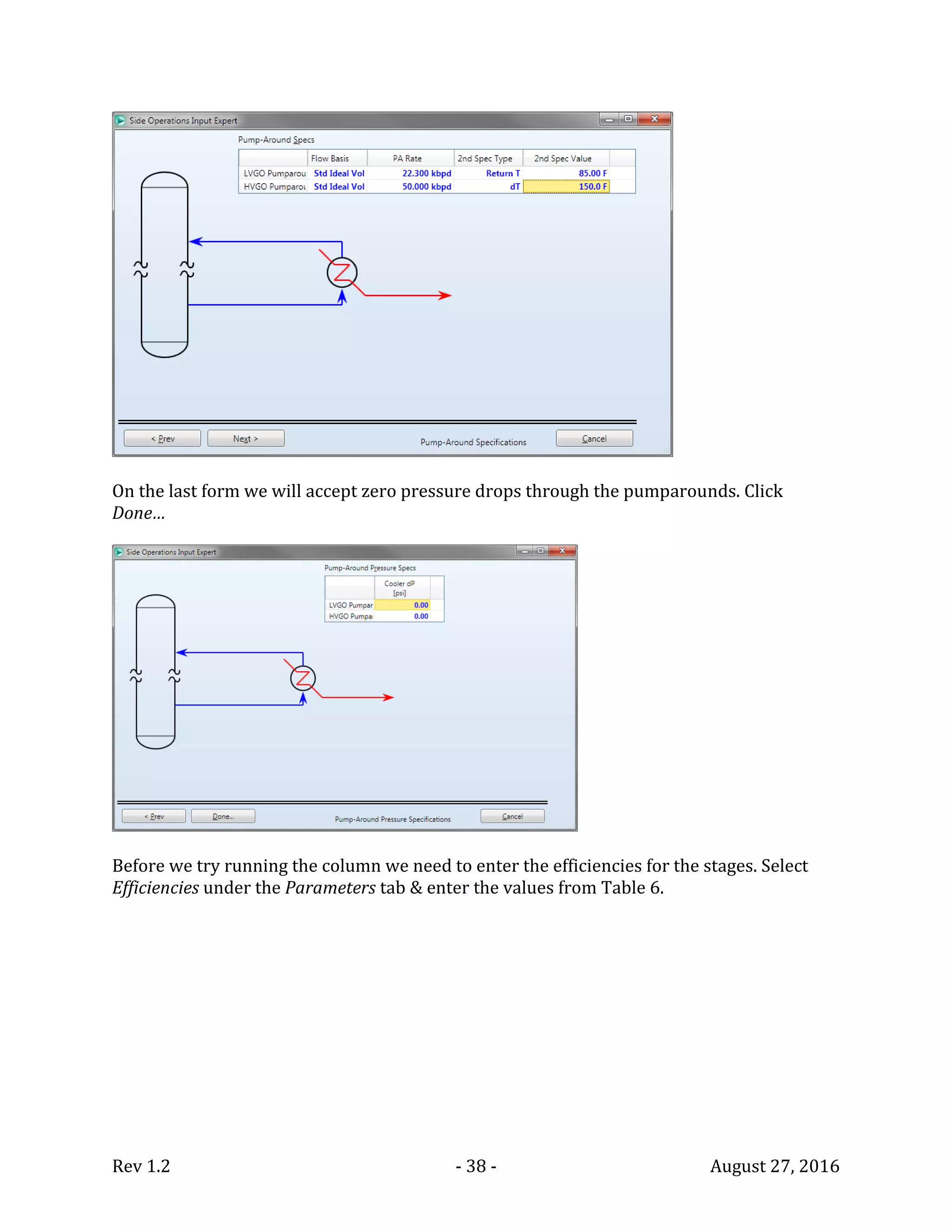
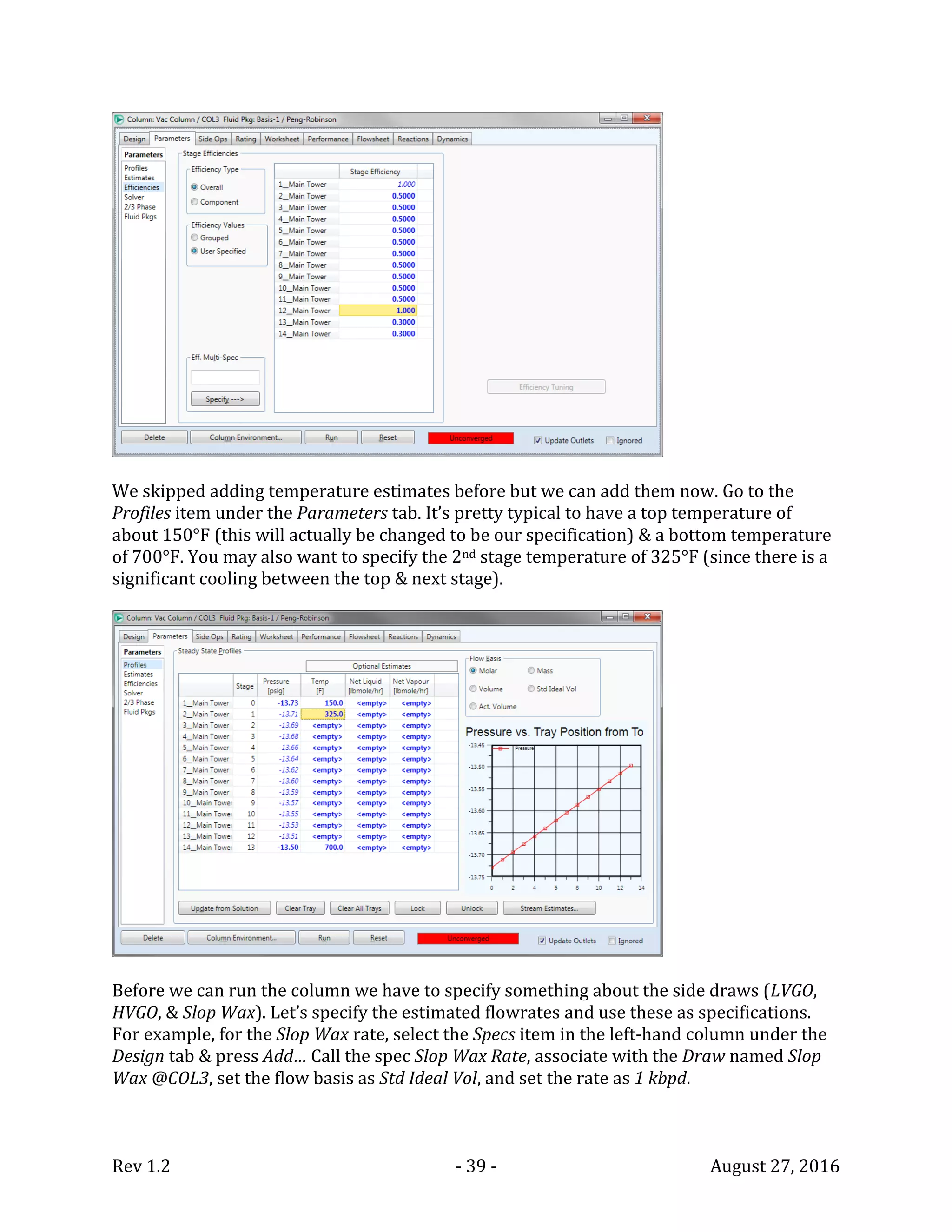
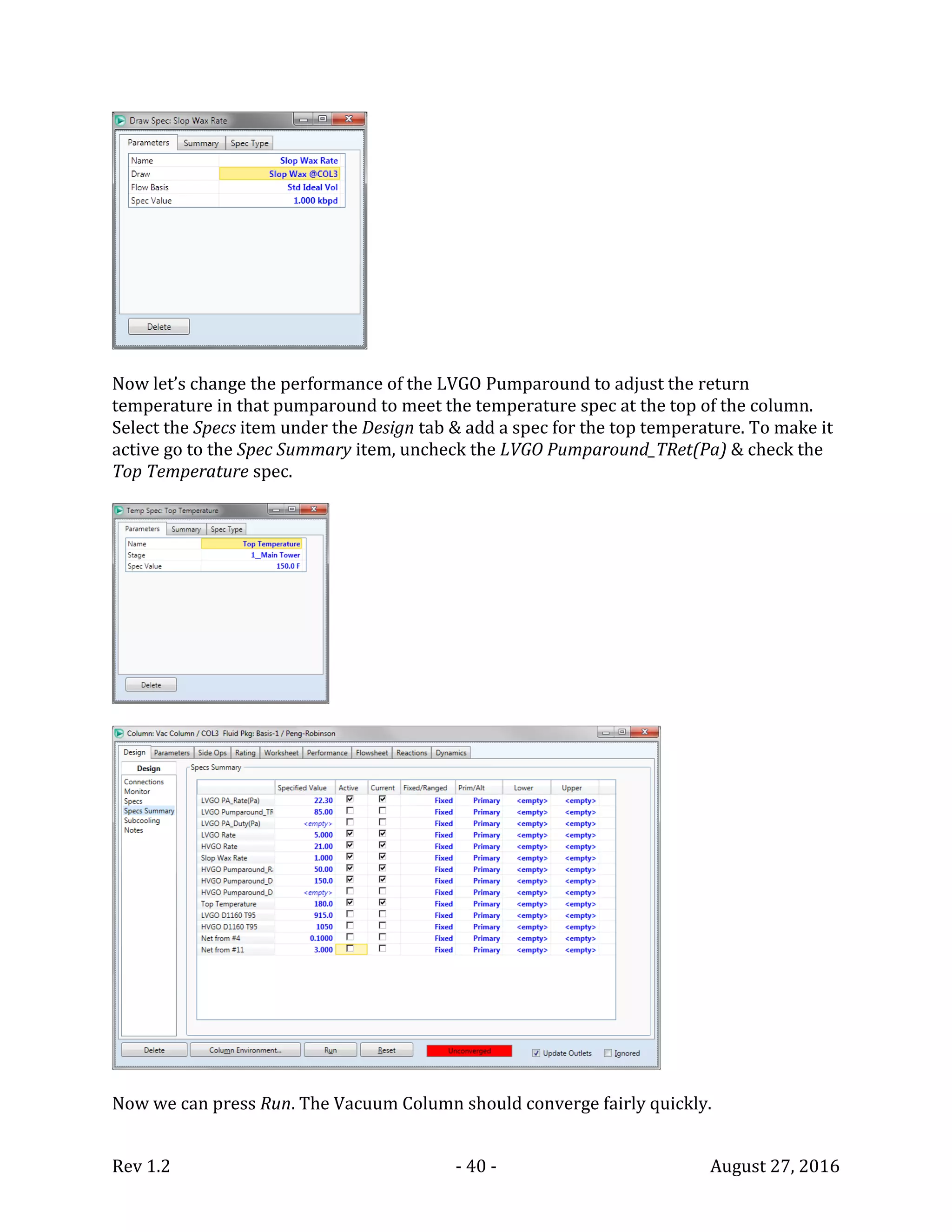
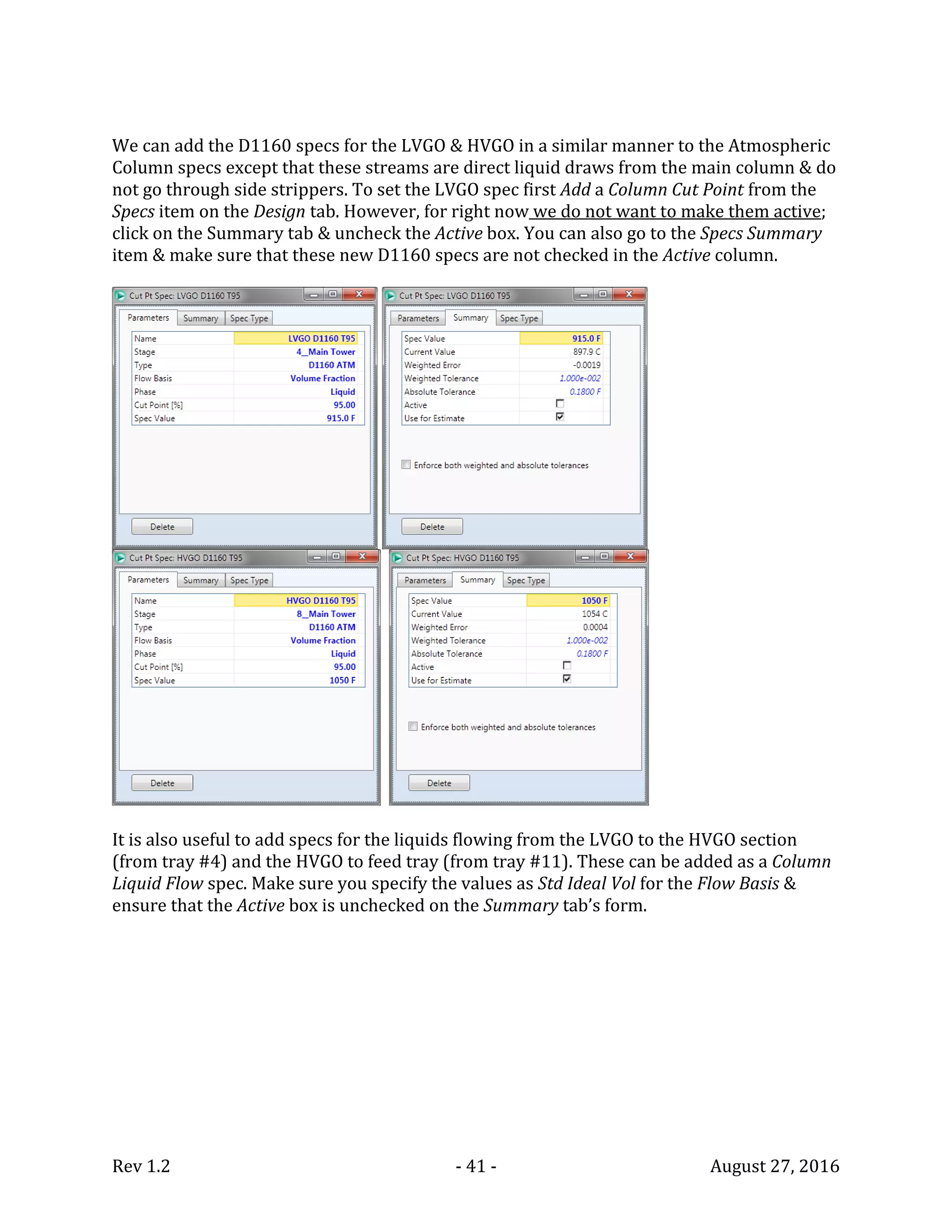
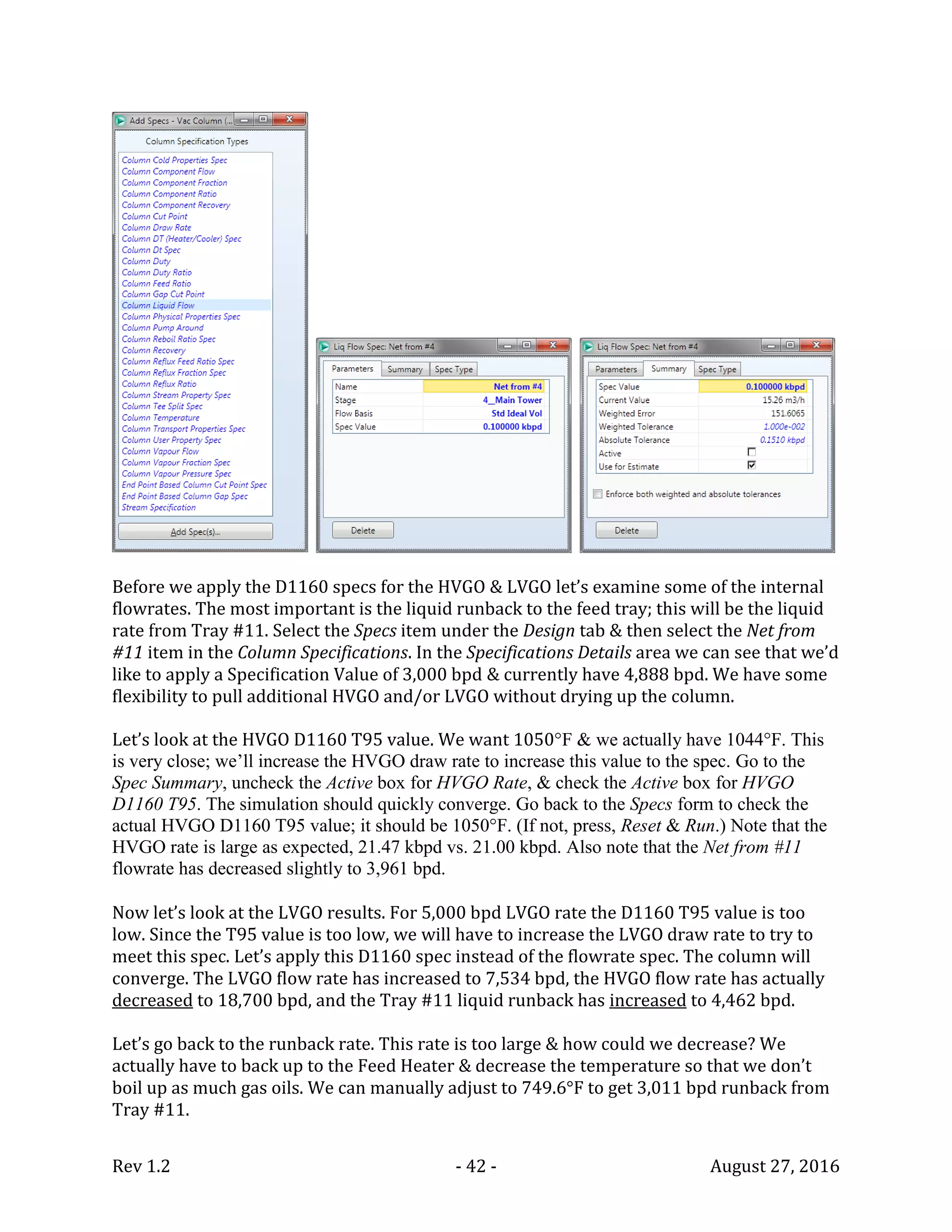
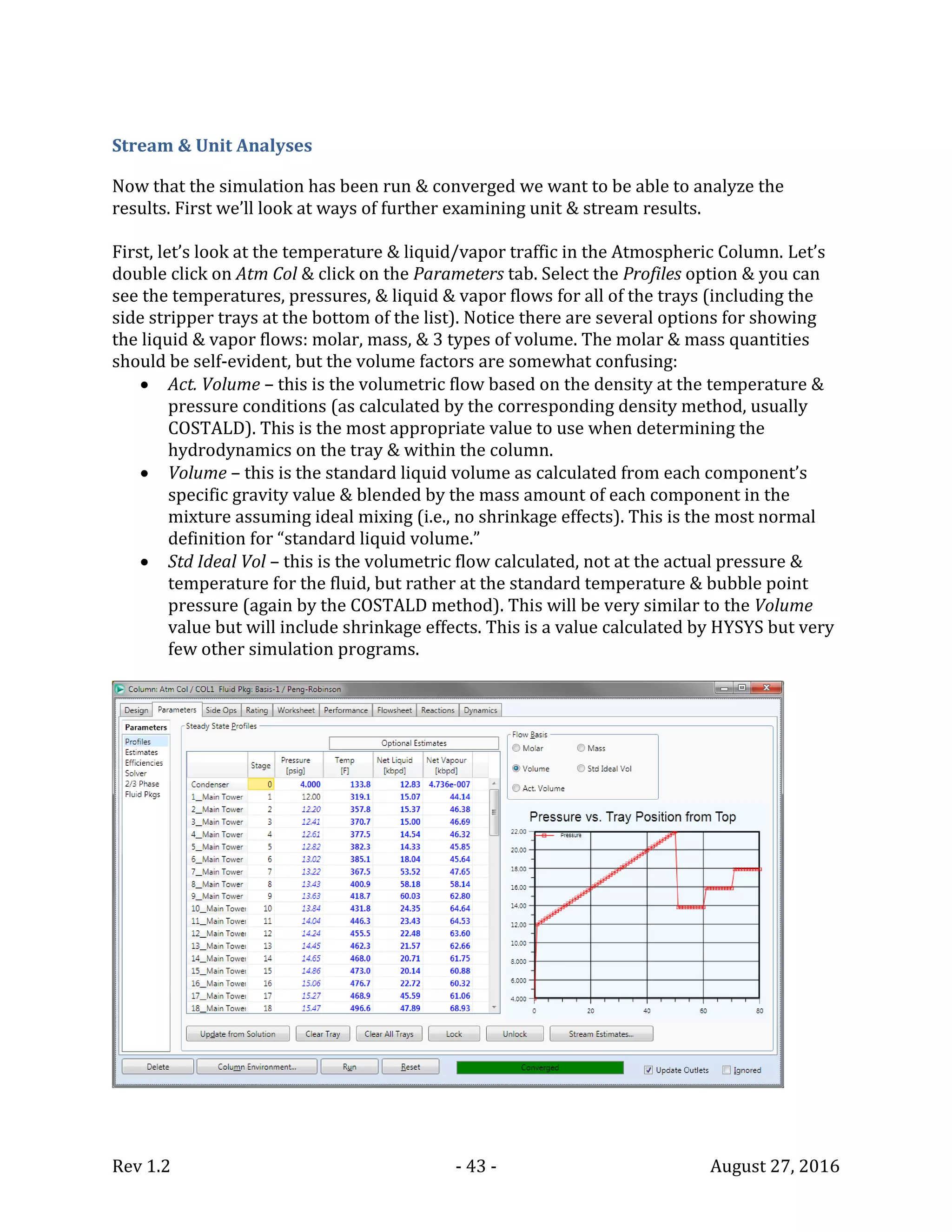
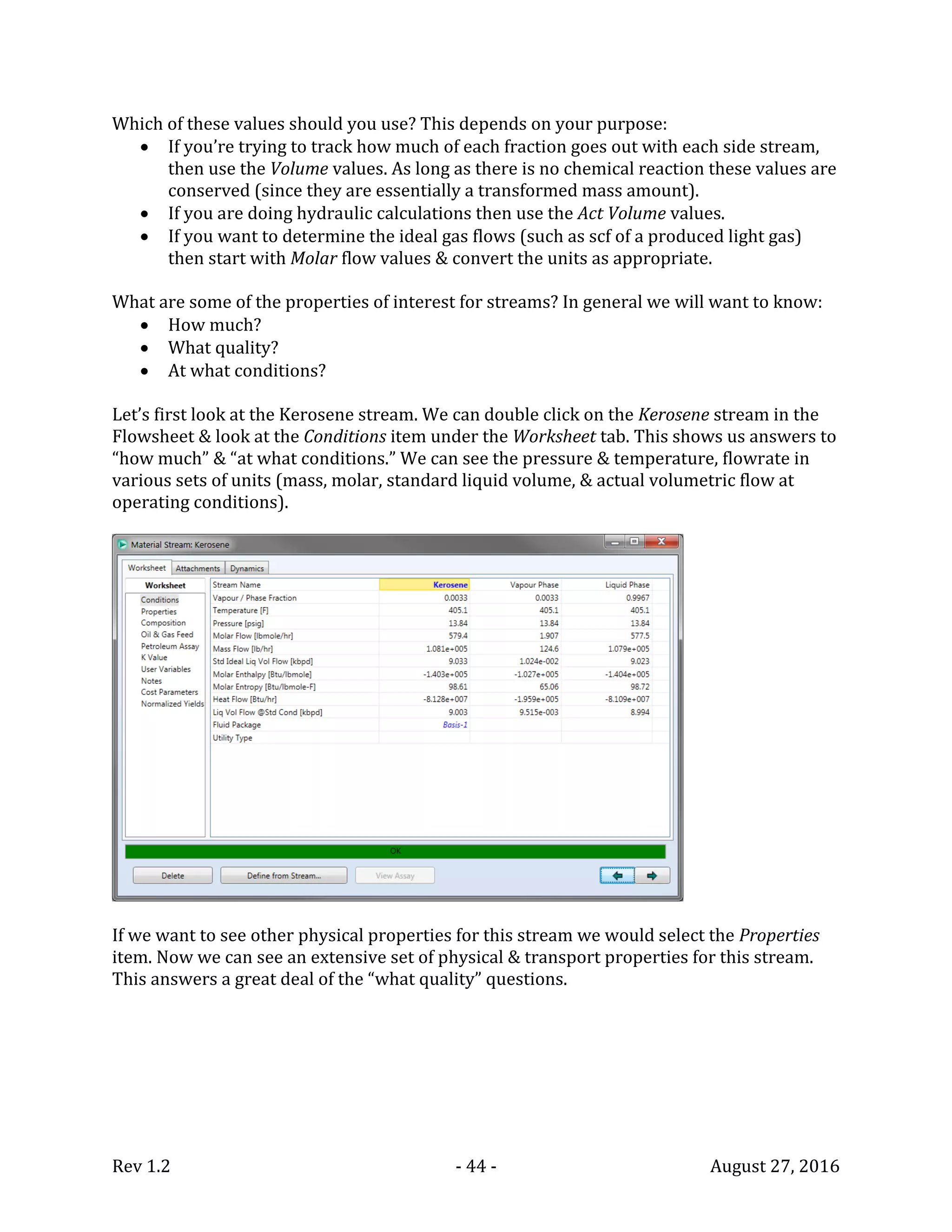
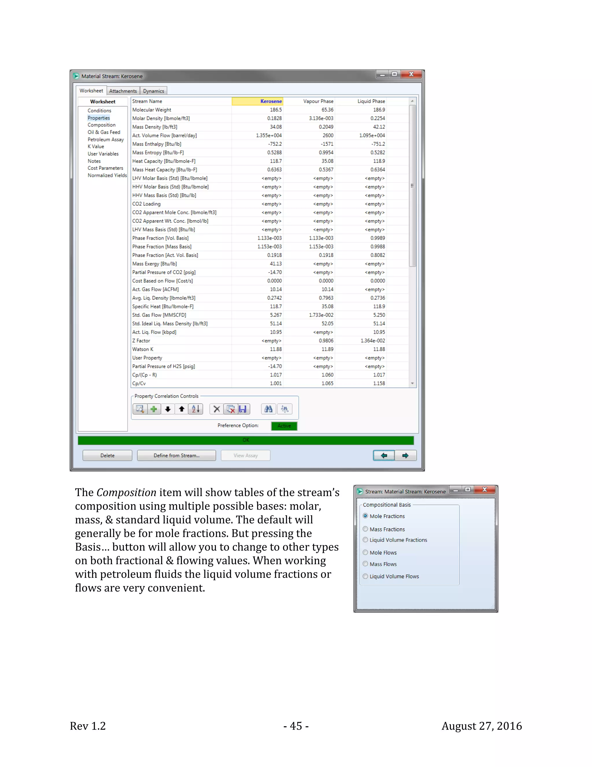
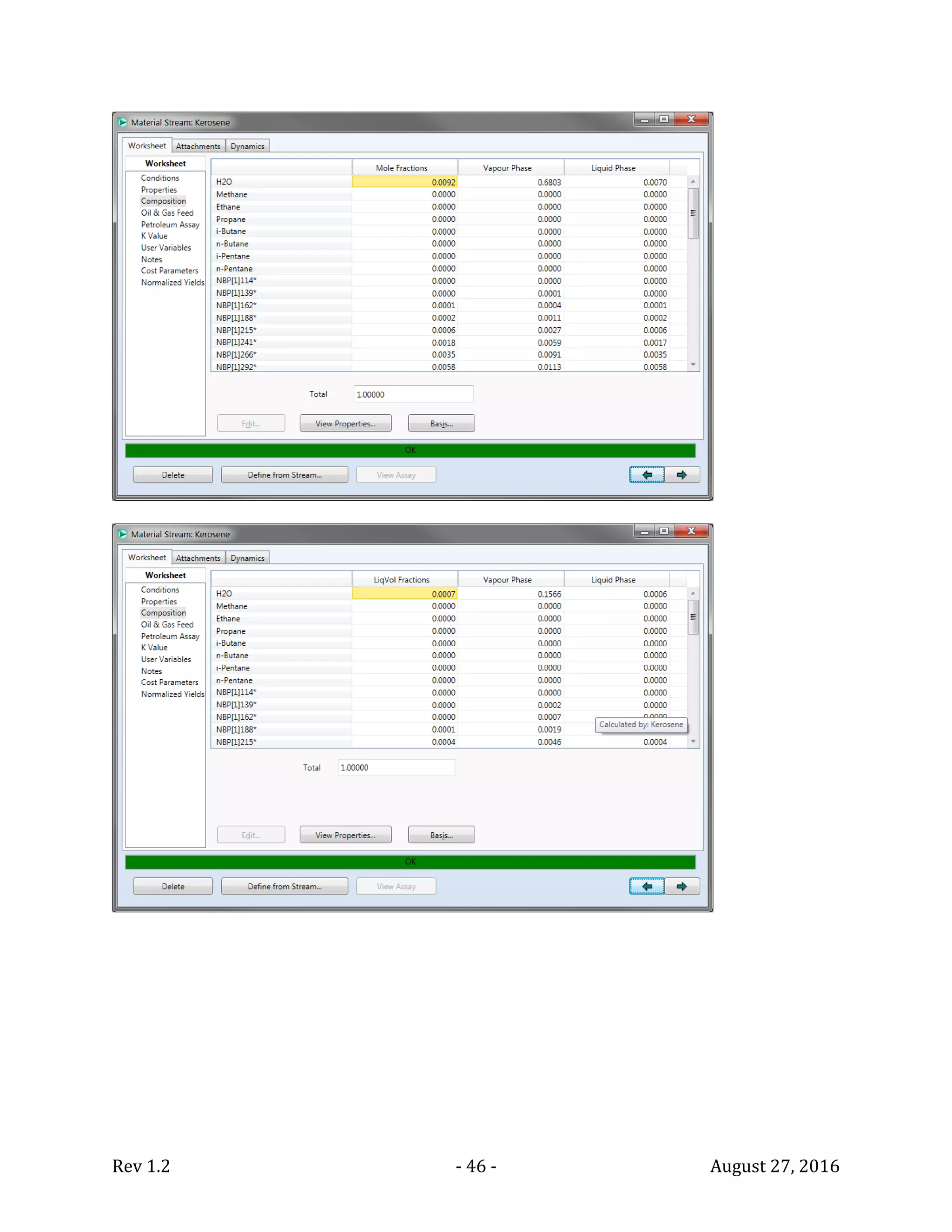
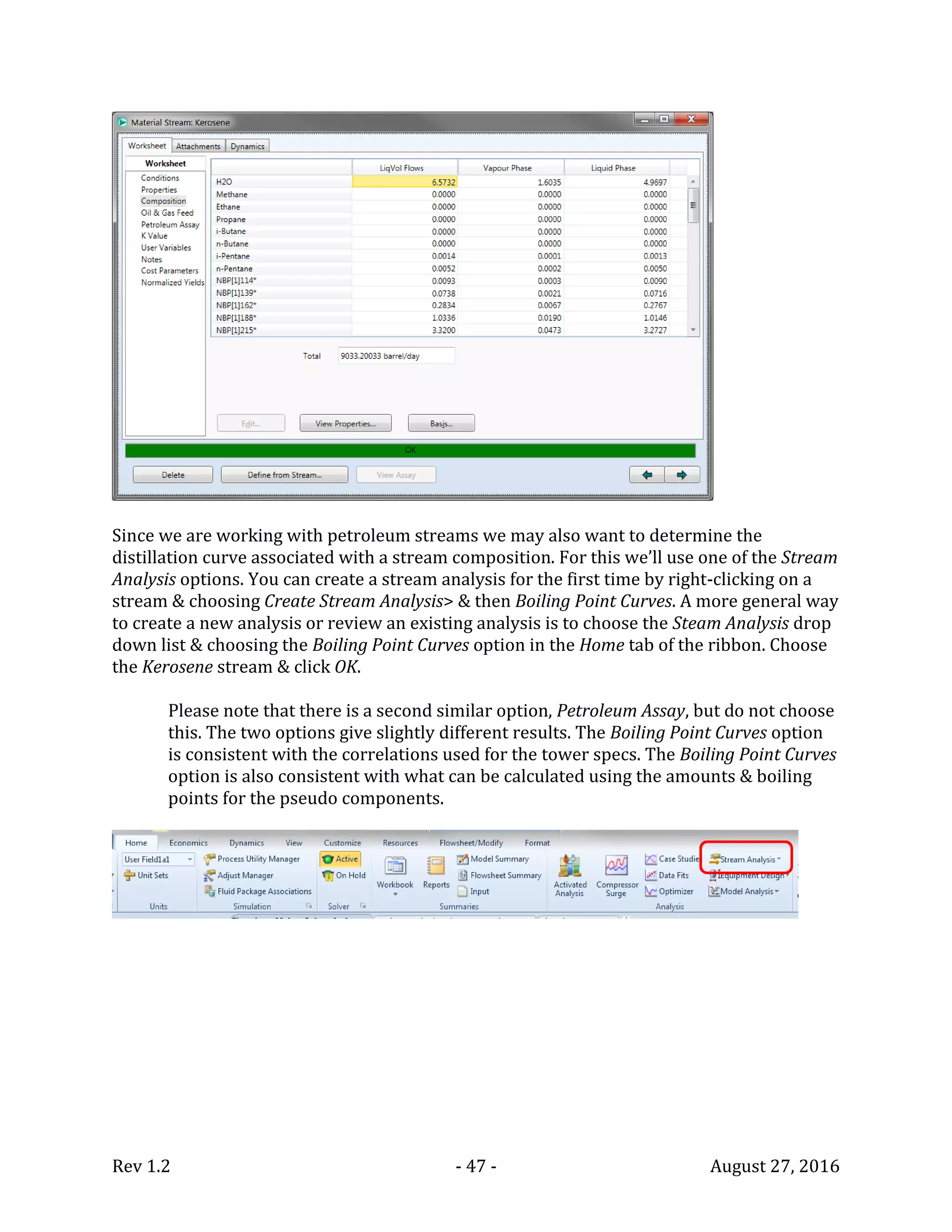
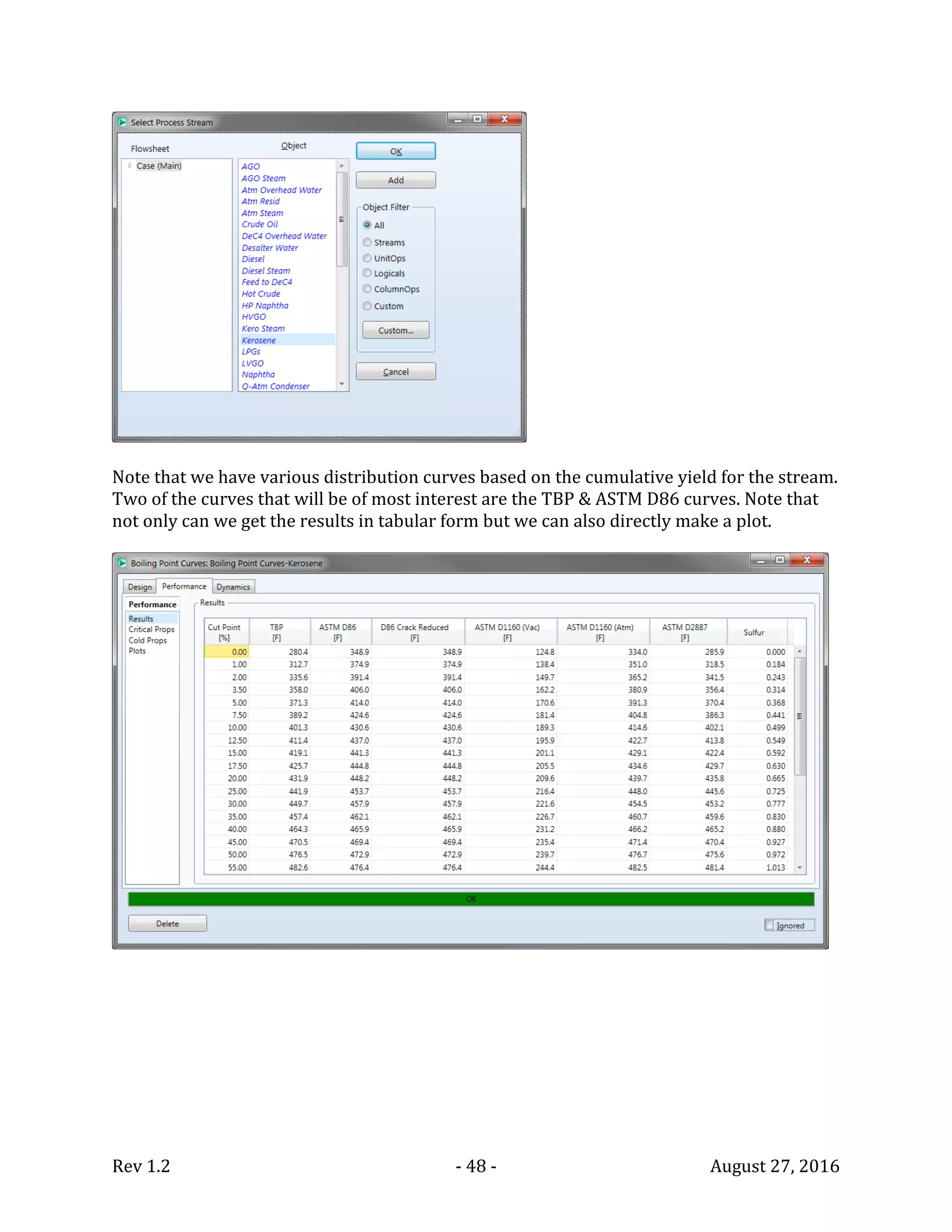
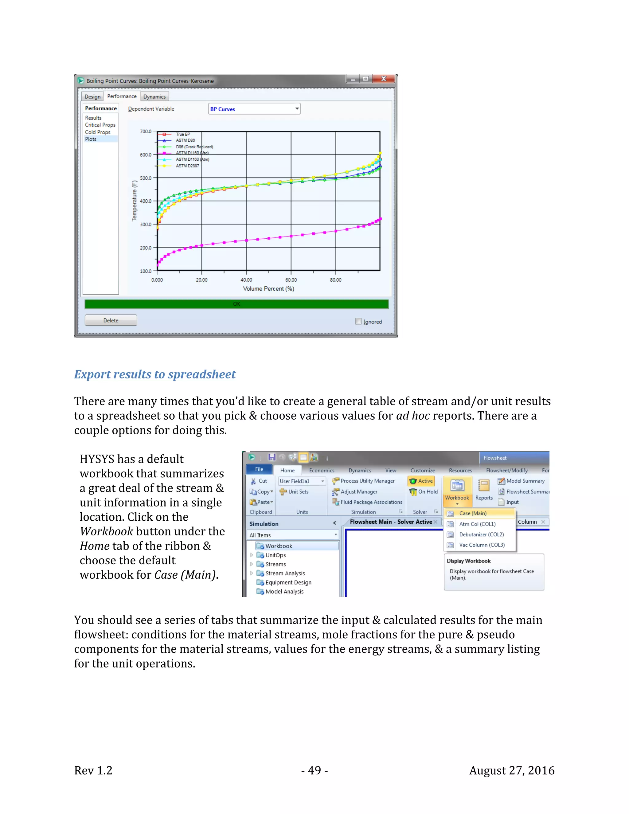
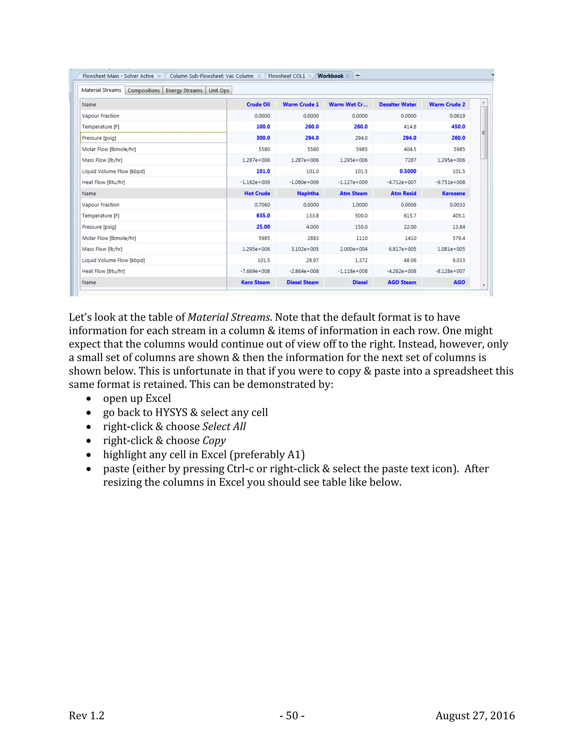
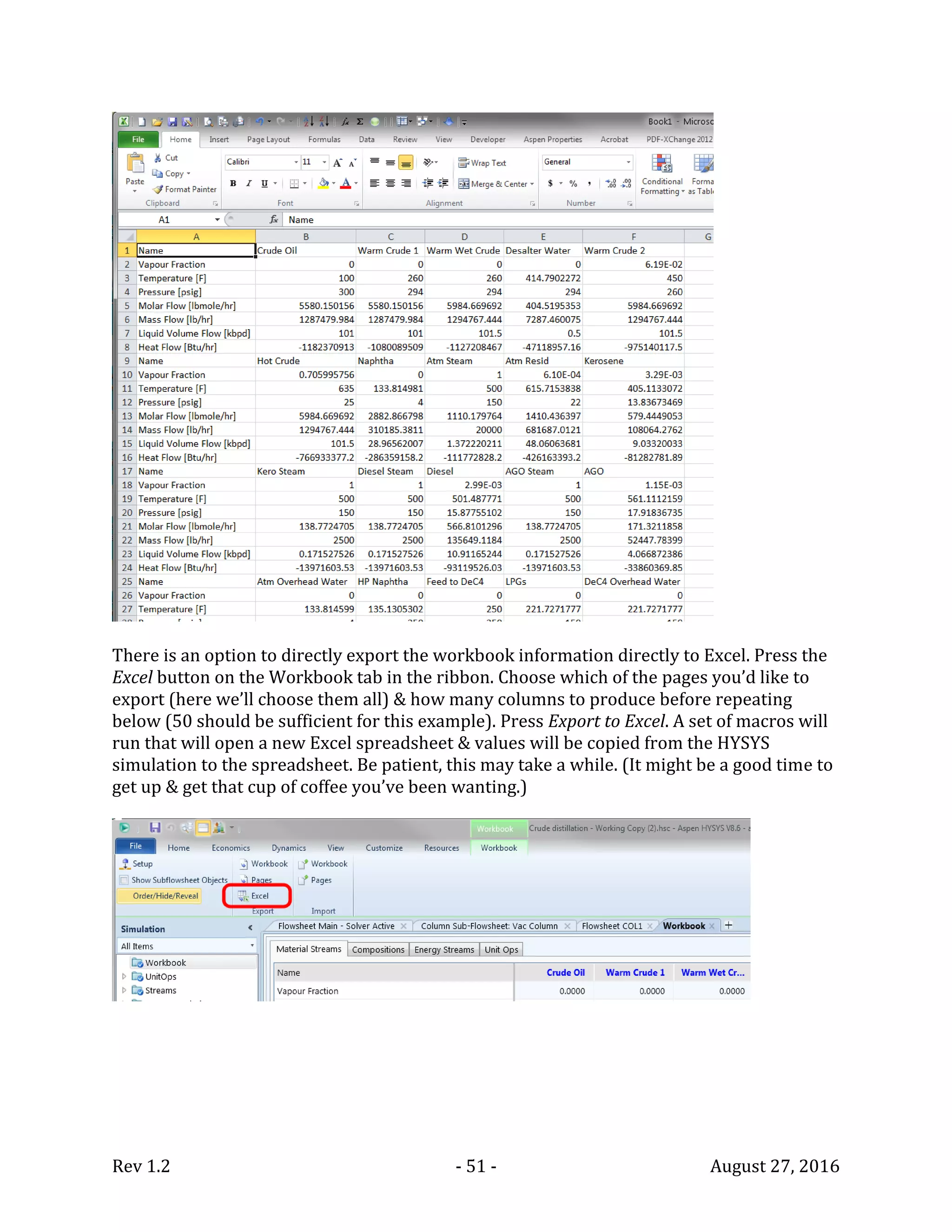
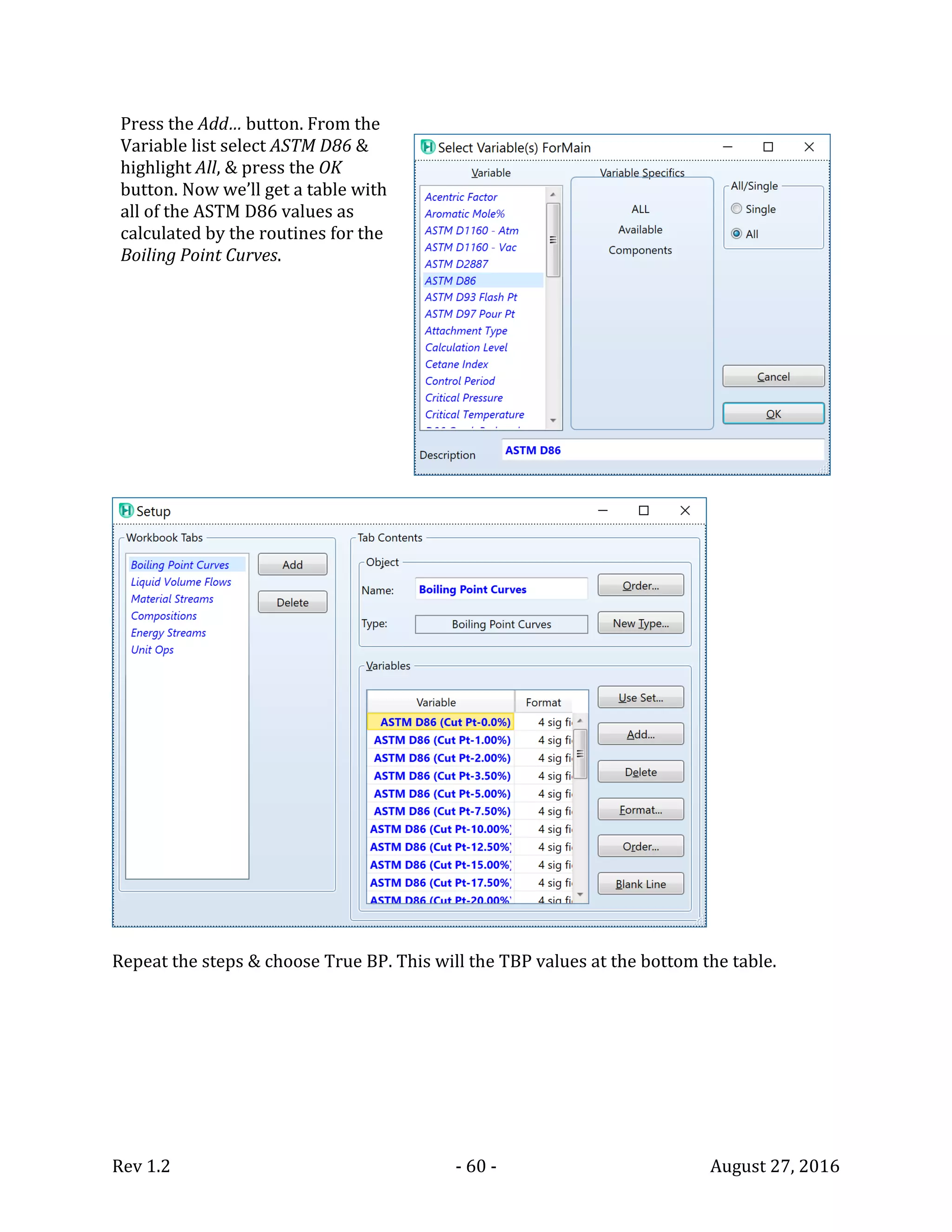


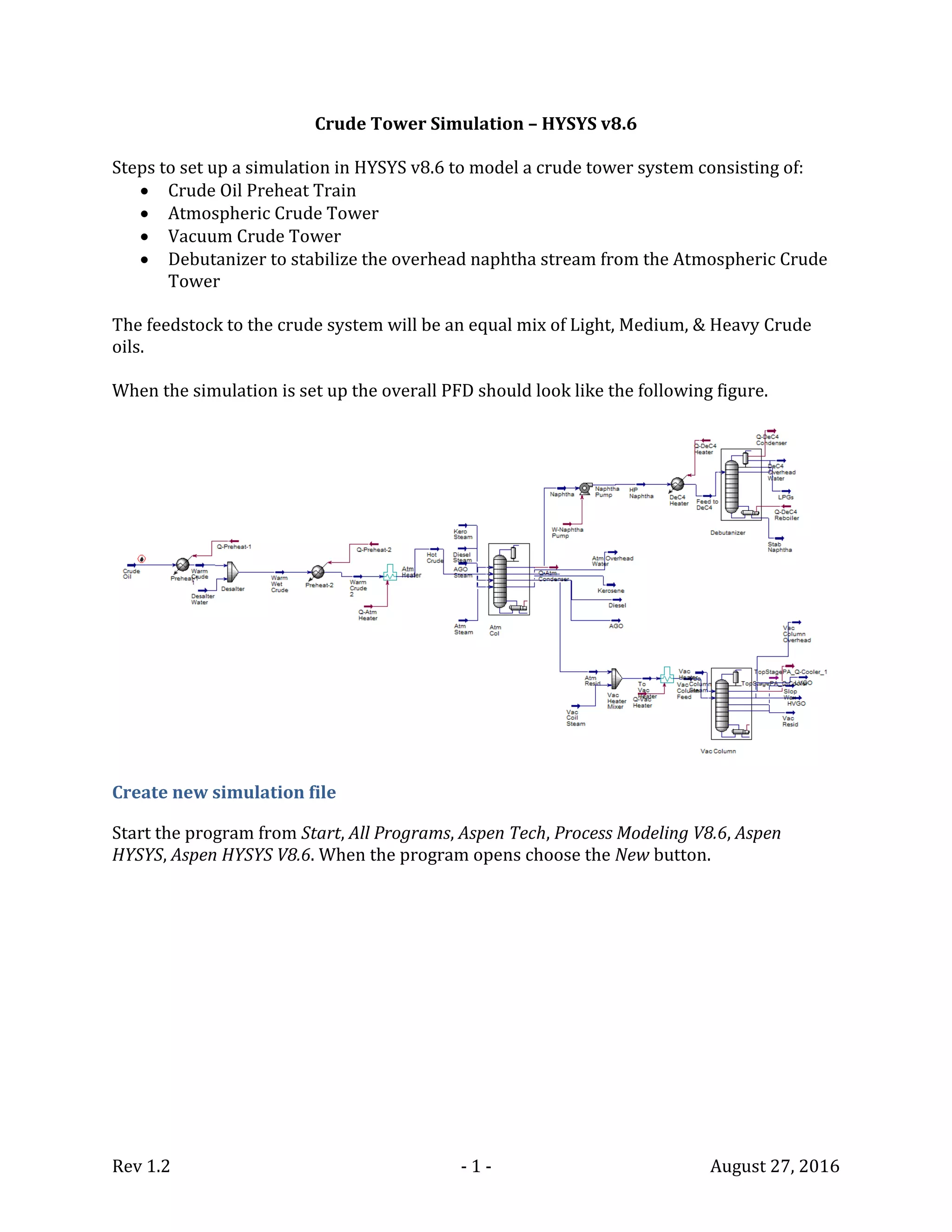
This document provides steps to set up a HYSYS simulation of a crude oil distillation system including a crude oil preheat train, atmospheric crude tower, vacuum crude tower, and debutanizer. The key steps include defining components and property packages, inputting assay data for light, medium, and heavy crude oils, characterizing the components, blending the crudes, installing the blend as the feedstock, and setting up the initial crude oil feed and preheat operations. The overall goal is to simulate a crude distillation system to produce stabilized naphtha and other products from a mixed crude oil feed.


