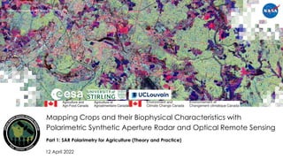
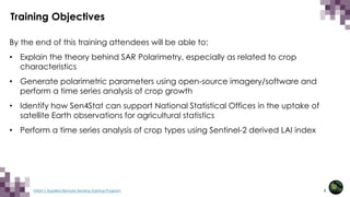
This document provides an overview of NASA's Applied Remote Sensing Training Program (ARSET) and its upcoming training on mapping crops and their biophysical characteristics using polarimetric synthetic aperture radar (SAR) and optical remote sensing. The training will consist of four sessions over four weeks covering SAR polarimetry theory, using the open-source Sen4Stat toolbox, a practical session with Sentinel-1, RCM, and SAOCOM SAR imagery, and time series analysis of crop growth monitoring. The goal is to increase the use of Earth observation data in decision making and applications such as agriculture.


![127
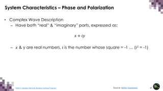
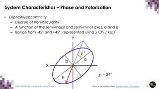
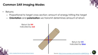
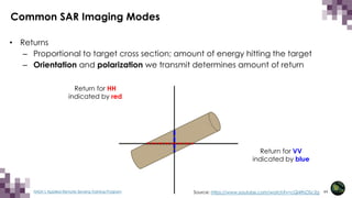
NASA’s Applied Remote Sensing Training Program
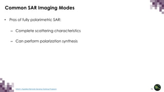
Polarimetry
• Coherent Decomposition
– Direct interpretation of the scattering matrix [S] is difficult
– Express [S] as the combination of responses from simpler (canonical) objects
– Coherent targets/point/pure targets: phase is known & predictable
– E.g., urban areas](https://image.slidesharecdn.com/cropmonitoringpart11-240328084750-c1916270/85/CropMonitoring-using-satellite-remote-sensing-127-320.jpg)
![128
NASA’s Applied Remote Sensing Training Program
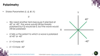
Polarimetry
• Incoherent Decomposition
– Speckle must characterize some targets statistically [C] and [T]
– Direct interpretation of the scattering matrix [C] and [T] difficult
– Incoherent targets
– E.g., forested areas](https://image.slidesharecdn.com/cropmonitoringpart11-240328084750-c1916270/85/CropMonitoring-using-satellite-remote-sensing-128-320.jpg)
![129
NASA’s Applied Remote Sensing Training Program
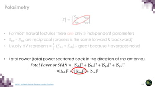
Polarimetry [C]
Coherent
Decomposition
W. Pauli (1900-1959)
E. Krogager (1990)
W. L. Cameron (1990)
[T]
Eigen-based
Decomposition
S. R. Cloude & E. Pottier
(1996-1997)
Eigenvectors/Eigenvalues Analysis
Model Based
Decomposition
Eigen-based/model
Based Decomposition
J. J. Van Zyl (1992)
[S] S. R. Cloude (1985)
W. A. Holm (1988)
A. Freeman (1992)
Source: Eric POTTIER](https://image.slidesharecdn.com/cropmonitoringpart11-240328084750-c1916270/85/CropMonitoring-using-satellite-remote-sensing-129-320.jpg)
![130
NASA’s Applied Remote Sensing Training Program
Polarimetry
• Cloude-Pottier Decomposition
– Eigenvector Eigenvalue based decomposition of [T]
– From this we get three secondary parameters
1) Entropy (H)
2) Anisotropy (A)
3) Mean Alpha angle (𝛼𝛼)](https://image.slidesharecdn.com/cropmonitoringpart11-240328084750-c1916270/85/CropMonitoring-using-satellite-remote-sensing-130-320.jpg)