This document discusses applying machine learning algorithms to three datasets: a housing dataset to predict prices, a banking dataset to predict customer churn, and a credit card dataset for customer segmentation. For housing prices, linear regression, regression trees and gradient boosted trees are applied and evaluated on test data using R2 and RMSE. For customer churn, logistic regression and random forests are used with sampling to address class imbalance, and evaluated using confusion matrix metrics. For credit card data, k-means clustering with PCA is used to segment customers into groups.

1. Applications of Data Mining methodologies in the
area of Predictive Analytics
Sarthak Khare
X18180485
School of Computing
National College of Ireland
Abstract— Since the advent of Alan Turing’s famous Turing
test, the area of Machine learning has grown leaps and bounds.
With the advancement in technology, complex machine learning
algorithms can now be performed on a personal computer in
very short periods of time. These advancements have really
paved the way for applying ML models to solve real world
challenges like predicting house prices, churn rate etc. This
study will deal with the applications of machine learning
algorithms in the area of predictive modelling to predict house
prices, customer churn and credit card user segmentation. For
this purpose, models such as Linear Regression, Regression tree,
Logistic regression, Random Forest and k-means clustering will
be applied to 3 different datasets and then evaluated by using
evaluation methods such as R2, RMSE, Confusion Matrix, ROC
on training and test set. Additionally, problems such as class
imbalance and dimensionality reduction, will also be tackled by
using sampling methods such as ROSE, SMOTE sampling and
PCA analysis respectively.
Keywords—Linear regression, Decision tree, Random forest,
k-means, ROSE sampling, SMOTE sampling, PCA, house price
prediction, customer churn, clustering.
I. INTRODUCTION
In this era of big data, with almost 2.5 quintillion bytes of data
being generated every day [1], it has become increasingly
important to train machines to gather any meaningful
information from this data. This process of extracting
meaningful insights from raw data is called data mining and
when we apply computer algorithms to make the computers
learn from this data and make predictions based on this, is
called machine learning.
Machine learning has become an important tool across all the
industries and businesses today, be it finance, marketing,
healthcare, real-estate etc., to tackle problems such as
customer churn, customer spending patterns, predicting
housing prices etc.
The aim of this project is to apply various machine learning
models (regression, classification and clustering) on three
different datasets to answer a business question specific to
each of these datasets and then choosing the best model by
evaluating the performance of the different models by using
the various model evaluating procedures such as R, adjusted
R2, RMSE, confusion matrix, ROC curve etc.
For this purpose, the following datasets have been sourced
from Kaggle, ‘House Sales in King County, USA’1, ‘Bank
customer churn modelling’ 2 , ‘Credit Card dataset for
clustering’3.
For each of these datasets, an attempt will be made to answer
the following research questions.
1 https://www.kaggle.com/harlfoxem/housesalesprediction
2 https://www.kaggle.com/barelydedicated/bank-customer-churn-modeling
A. Which is the best regression model to predict the house
sale prices for the houses in King County, USA, using various
different attributes such as property size, number of
bedrooms, bathrooms etc.?
B. Using different classification algorithms, can we predict if
a customer will leave the bank or not? Based on customer’s
credit score, gender, age etc.
C. Based on customer’s credit card information, can we use
clustering algorithms to segment customers into different
groups, to define a marketing strategy to target each group?
II. RELATED WORK
Due to the boom in the real-estate industry in the recent years,
there have already been many previous studies which have
attempted to tackle the question of predicting the house prices
using machine learning models. One such study conducted by
D.Phan [2] uses Polynomial Regression, SVM, neural
network and regression tree against linear model acting as a
baseline to make prediction on the Australian housing market
data. Here SVM combined with PCA gives the best results.
Another thing of note in the above study was the use of log
transformation on the predicted variable as it was highly
skewed. In another study conducted by S.Lu et al [3], they
apply feature engineering by using log transformations of
skewed features and using techniques like one-hot encoding
and binning and finally applying Ridge, Lasso and Gradient
boosting to get the best result with a hybrid of Lasso and
gradient boosting.
Viktorovich et al. in their paper [4] again have used log
transformation to transform the house price variable and have
further used k-fold cross validation along with the classic
regression techniques to get better results on a small sample.
Banerjee et al. [5] have tackled the problem of house price in
a different way, by considering it a classification problem and
predicting if the price will increase or decrease based on
certain features. They have also used VIF (Variance
Influence Factor) to analyze which are the most important
features, when it comes to analyzing the real-estate market.
As a lot of studies have showed, it is important to tackle the
skewness of the variables by transforming them using log or
square-root or other transformation techniques to get better
results, the predicted variable (house price) would need to be
transformed first by taking its log. Also, most of the studies
above have made use of some advance DM techniques like
ANN, SVM, Random Forest etc. which have very high
computational costs, this study will focus on applying simple
models like Multiple linear regression and regression trees to
3 https://www.kaggle.com/arjunbhasin2013/ccdata

2. see if we can achieve same level of results for the housing
dataset.
Customer retention is one of the topmost priority of any
business, hence a lot of literature is available on the topic of
customer churn prediction. Jing et al. [6] in their paper have
applied various classification methods such as SVM, Logistic
regression, Decision tree and Naïve Bayes and found SVM to
be the best model to predict customer churn. Yadav S. et al.
[7] have used feature engineering methods, such as ‘brute
force’, where a large number of categorical variable were
combined into 2 categories, and ‘one hot encoding’, where
each categorical variable was assigned 1 or 0 as values. The
model performed better with one-hot encoding.
Nie et al. [8] talk about the importance of understanding the
features contributing to the model when dealing with
customer churn, so as to have a better understanding of the
factors that have an effect on churn. For this reason, they have
selected Logistic regression and Regression tree models as
their model of choice, for doing churn analysis.
Almost all of the studies in the area of churn prediction talk
about the problem of class imbalance. Class imbalance occurs
when the numbers of one class is significantly higher than the
number of the other class. [9] To tackle this problem,
Sampling techniques such as ROSE (Random Over-
Sampling Examples) [10] and SMOTE (Synthetic Minor
Over-Sampling Technique) [11] have been proposed. ROSE
uses smoothed bootstrap approach to generate artificially
balanced samples. Phetlasy et al. [12] achieved an increase of
over 15% in their model’s sensitivity by using SMOTE
sampling. Based on this, this report will make use of these 2
sampling techniques to address the issue of class imbalance
in the predicted variable and apply classification models such
as Logistic regression and Random forest and validate on the
basis of not just accuracy but sensitivity and specificity of the
models.
Customer segmentation is an important marketing strategy
used in all the industries. In these 2 research papers, [13] [14]
authors use the RFM (Recency, Frequency, Monetary) score,
which is based on customer visits, the frequency of customer
visits and the revenue earned, and k-means clustering
algorithm to segment customers. Lei et al. [15] have made use
of k-means clustering to segment credit card users by using
top 3 features by using PCA analysis and then proceeded to
do predictive analytics by using models such as C5.0 and
neural networks to segment any future users to these clusters.
As observed from the literature, k means is the most popular
algorithm for customer segmentation, so this study will make
use of k-means combined with PCA to segment the credit
card users.
III. METHODOLOGY
KDD (Knowledge Discovery in Databases) has been chosen
as the data mining methodology for this project. KDD
generally consists of five major steps, each of which will be
discussed in terms of this project.
4 http://www2.cs.uregina.ca/~dbd/cs831/notes/kdd/1_kdd.html
Fig.1 KDD model4
A. Data Selection
Three different datasets for this study were sourced from
Kaggle.
1. For predicting house prices by applying regression
models, ‘House Sales in King County, USA’ dataset
has been sourced from Kaggle. This dataset contains
more than 10000 records and has 21 attributes in all
with the ‘price’ attribute having quantitative price
values and being the predicted variable. Figure 2 below
shows the data dictionary for the dataset.
Fig. 2
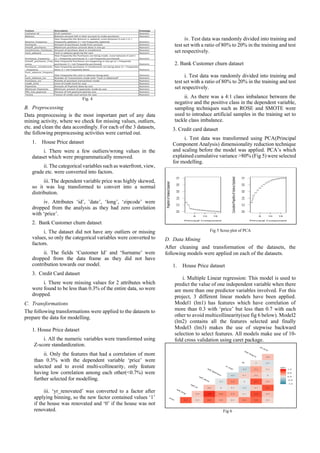
2. For determining the customer churn rate in a bank by
applying classification algorithms, ‘Bank customer
churn modelling’ dataset has been sourced from
Kaggle. This dataset contains 10000 records and has 14
attributes. ‘Exited’ is the predicted variable with values
1 for ‘exited’ and 0 for ‘not-exited’. Figure 3 below
shows the data dictionary for the dataset.
Fig. 3
3. For grouping credit card users into different segments
for defining a marketing strategy based on similar
attributes of those groups, ‘Credit Card dataset for
clustering’ has been sourced from Kaggle. This dataset
contains almost 9000 records and 18 behavioral
attributes of credit card user data collected over a period
of 6 months. Figure 4 below shows the data dictionary
for the dataset.

3. Fig. 4
B. Preprocessing
Data preprocessing is the most important part of any data
mining activity, where we check for missing values, outliers,
etc. and clean the data accordingly. For each of the 3 datasets,
the following preprocessing activities were carried out.
1. House Price dataset
i. There were a few outliers/wrong values in the
dataset which were programmatically removed.
ii. The categorical variables such as waterfront, view,
grade etc. were converted into factors.
iii. The dependent variable price was highly skewed,
so it was log transformed to convert into a normal
distribution.
iv. Attributes ‘id’, ’date’, ‘long’, ‘zipcode’ were
dropped from the analysis as they had zero correlation
with ‘price’.
2. Bank Customer churn dataset
i. The dataset did not have any outliers or missing
values, so only the categorical variables were converted to
factors.
ii. The fields ‘Customer Id’ and ‘Surname’ were
dropped from the data frame as they did not have
contribution towards our model.
3. Credit Card dataset
i. There were missing values for 2 attributes which
were found to be less than 0.3% of the entire data, so were
dropped.
C. Transformations
The following transformations were applied to the datasets to
prepare the data for modelling.
1. House Price dataset
i. All the numeric variables were transformed using
Z-score standardization.
ii. Only the features that had a correlation of more
than 0.3% with the dependent variable ‘price’ were
selected and to avoid multi-collinearity, only feature
having low correlation among each other(<0.7%) were
further selected for modelling.
iii. ‘yr_renovated’ was converted to a factor after
applying binning, so the new factor contained values ‘1’
if the house was renovated and ‘0’ if the house was not
renovated.
iv. Test data was randomly divided into training and
test set with a ratio of 80% to 20% in the training and test
set respectively.
2. Bank Customer churn dataset
i. Test data was randomly divided into training and
test set with a ratio of 80% to 20% in the training and test
set respectively.
ii. As there was a 4:1 class imbalance between the
negative and the positive class in the dependent variable,
sampling techniques such as ROSE and SMOTE were
used to introduce artificial samples in the training set to
tackle class imbalance.
3. Credit card dataset
i. Test data was transformed using PCA(Principal
Component Analysis) dimensionality reduction technique
and scaling before the model was applied. PCA’s which
explained cumulative variance >80% (Fig 5) were selected
for modelling.
Fig 5 Scree plot of PCA
D. Data Mining
After cleaning and transformation of the datasets, the
following models were applied on each of the datasets.
1. House Price dataset
i. Multiple Linear regression: This model is used to
predict the value of one independent variable when there
are more than one predictor variables involved. For this
project, 3 different linear models have been applied.
Model1 (lm1) has features which have correlation of
more than 0.3 with ‘price’ but less than 0.7 with each
other to avoid multicollinearity(see fig 6 below). Model2
(lm2) contains all the features selected and finally
Model3 (lm3) makes the use of stepwise backward
selection to select features. All models make use of 10-
fold cross validation using caret package.
Fig 6

4. ii. Regression tree: Regression trees are a form of
decision trees where the outcome variable has
continuous values. In this project, simple regression tree
and gradient boosted regression tree models have been
used using the rpart and gbm packages. As decision tree
don’t need normalization, train and test data have not
been normalized, only the predicted variable ‘price’ has
been log transformed. Model1 (tm1) is a simple
regression tree model, Model 2 (tm2) has been tuned
using hyper parameters, minsplit and maxdepth. Model
3 (tm_gbm) is gradient boosted model. All the models
have used 10-fold cross validation using caret package.
2. Bank Customer churn dataset
i. Logistic Regression: Logistic regression is used for
classification problems where the variable has binary
outcome i.e. yes/no, pass/fail, that can be coded as ‘1’ or
‘0’. [16] It typically calculates the probability of the
outcome and based on that probability of occurrence,
transforms the dependent variable to the values 0 or 1. In
this dataset, 3 logistic regression models with different
training samples have been used, by using the ‘glm’
package in R. Model1 (glm1) uses the original training
data, Model2(glm2_rose) uses the training data with
ROSE sampling applied to it and finally Model3
(glm3_smote) uses the training data with SMOTE
sampling applied to it. All the models use 10-fold cross
validation using the caret package.
ii. Random Forest: A random forest as its name
suggests is an ensemble of individual decision trees where
each tree spits out a class prediction and the predicted
class with the most number of votes is selected. [17]
Similar to logistic regression, 3 random forest models
have again been used for this dataset using the ‘ranger’
package. Model1 (rf1) uses the original training data,
Model2(rf2_rose) uses the training data with ROSE
sampling applied to it and finally Model3 (rf3_smote)
uses the training data with SMOTE sampling applied to
it. All the models use 10-fold cross validation using the
caret package.
3. Credit card datset:
i. K-means Clustering: k means clustering is a type
of unsupervised learning model, where the predictor class
is not known. It works by partitioning ‘n’ observations
into ‘k’ clusters by assigning each observation to the
cluster with the nearest mean (centroid of the cluster).
[18] After assigning all the observations into k-clusters,
the centroids of the clusters are re-calculated by averaging
out all the points in the cluster. [19] After re-calculating
the new centroids, all the observations are again re-
assigned to the closest centroid cluster. This process is
repeated until there are no new-reassignments to be made.
[19]. For this dataset, ‘kmeans’ from the base package has
been used iteratively 20 times to find the most optimal
value of k.
E. Interpretation/Evaluation:
The last part of the KDD process is the evaluation of the
models. This will be covered in the next section.
IV. EVALUATION
After applying different supervised and unsupervised
techniques to our dataset, we will now evaluate them.
Regression models will be evaluated using the R2 and RMSE
metrics on the test data. Classification models will be
evaluated using the Confusion matrix values of accuracy,
sensitivity, specificity and the ROC curve value AUC on the
test data. For clustering, within sum of squares metric will be
used to calculate the optimal value of k.
1. House Price Dataset:
We can evaluate the performances of the different
regression models on the test set using the R2 and RMSE
metrics. R2 explains the variance in the response variable of
the test data and RMSE or the Root Mean Squared Error,
explains the standard deviation of the predicted data points
form the actual data points. R2 should be high(close to 1) and
RMSE should be low for a good model. From figure 7, we can
see, Gradient boosted regression tree model (tm3) out
performs all the other models with a R2 value of 0.88 and
RMSE value of 0.19. The linear models also perform well
with R2 and RMSE values being quite close to each other.
Among the linear models, model lm2, with all the features
selected performs the best, however, it’s performance is
incredibly close to lm3 model’s performance, which was
selected using stepwise backward elimination. So, we’ll chose
lm3 as the best linear model as it takes less features to explain
the model. Lm3’s formula and regression coefficients can be
seen in figure 8.
Fig. 7
Fig 8
Although the performance of the regression tree models tm1
and tm2 is not that great in comparison, it still can help us with
understanding the features on which the decisions to form the
models were based (figure 9).

5. Fig. 9
2. Customer Churn Dataset:
We can evaluate the performance of different classification
models using the AUC of ROC curve and the Accuracy,
Sensitivity and Specificity values obtained from the confusion
matrix of different models. Figure 10 contains all these
metrics on the test set of customer churn dataset.
From figure 10, we can observe, glm2_rose is the best model
in terms of the AUC but model rf1 is the best in terms of
accuracy among all the other models. However, considering,
the predicted variable ‘Exited’ has a 4:1 class imbalance of
negative to positive classes, sensitivity or the True Positive
Rate(TPR) becomes the most important metric to select the
best performing model. Going by this, we can see ROSE
sampled models have the best TPR/sensitivities followed by
SMOTE sampled models. Without sampling, we get the best
accuracies for the models but as expected, the TPRs are really
low.
Fig 10
Figure 11 below shows the ROC curves for all of the models.
Here again we can see the ROSE models perform the best,
followed by the SMOTE models and finally models with no
sampling.
Fig. 11
3. Credit Card Dataset:
Evaluating the performance of a clustering model can be done
by selecting the optimal number of clusters(k) using the elbow
method. Mostly domain knowledge is needed to select the
most optimal value of k however, using the elbow method we
can calculate the within sum of squares of each cluster and
select the k where the graph forms an elbow or the decrease in
WSS as k increase is minimal.
From figure 12, a value of 8 seems to be the most optimal so
k has been set to 8 for creating a model.
Fig 12
Figure 13 is the plot of PC1 and PC2 (principal components)
grouped by clusters from which we can get an idea of the
groupings.
Fig. 13
Figure 14 below shows the summary of the mean values of all
the variables grouped by their clusters. Based on this we can
see, cluster 8 has really high values in almost all the variables,
so we may assume cluster 8 comprises of high spenders who
also do a lot of high end transactions. By doing a similar
analysis a domain expert should be able to do customer
segmentation based on these results.
Fig 14

6. V. CONCLUSION AND FUTURE WORK
In this project we applied supervised and unsupervised
machine learning techniques on different unrelated datasets
and evaluated the performance of each of those models on the
test data.
For our regression models on the house price data, we
observed which features are the most important when it
comes to the real estate market by using the insights from our
linear models while getting the best predictive results from
the boosted regression tree model.
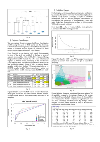
For our customer churn data, we saw the effect of class
imbalance on the selection of a model and chose logistic
regression rose model as the best performing model based on
the sensitivity of the model rather than the accuracy.
For clustering, we formed 8 clusters based on the within sum
of squares of each of the cluster and using the summary table
of the mean values of each variable by cluster, we were able
to understand the different customer types.
In the future, there is scope to make use of even more
supervised and unsupervised machine learning models on
these datasets to make an even better comparison and to try
and improve the performances of these models by using
parameter tuning.
VI. REFERENCES
[1] [Online]. Available:
https://www.forbes.com/sites/bernardmarr/2018/05/21/how-
much-data-do-we-create-every-day-the-mind-blowing-stats-
everyone-should-read/#32a1483360ba.
[2] D. Phan, "Housing Price Prediction using Machine Learning
Algorithms: The Case of Melbourne City, Australia," in
2018 International Conference on Machine Learning and
Data Engineering (iCMLDE), Sydney,Australia, 2018.
[3] S. Lu, Z. Li and Z. Qin, "A Hybrid Regression Technique
for House Prices Prediction," in 2017 IEEE International
Conference on Industrial Engineering and Engineering
Management (IEEM), 2017.
[4] P. Viktorovich, P. Aleksandrovich and I. Leopoldovich,
"Predicting Sales Prices of the Houses Using Regression
Methods of Machine Learning," in 2018 3rd Russian-
Pacific Conference on Computer Technology and
Applications (RPC), 2018.
[5] D. Banerjee and S. Dutta, "Predicting the Housing Price
Direction using Machine Learning Techniques," in IEEE
International Conference on Power, Control, Signals and
Instrumentation Engineering (ICPCSI-2017), 2017.
[6] Z. Jing and D. Zing-Hua, "Bank Customer Churn Prediction
Based on Support Vector Machine: Taking a Commercial
Bank’s VIP Customer Churn as the Example," in IEEE,
2008.
[7] S. Yadav, A. Jain and D. Singh, "Early Prediction of
Employee Attrition using Data Mining Techniques," in
IEEE, 2018.
[8] G. Nie and W. Rowe, "Credit card churn forecasting by
logistic regression and decision tree," Expert Systems with
Applications, 2011.
[9] B.-e.-d. Mohammed, t. Perry and E. Teitei, "Biased Random
Forest For Dealing With the Class Imbalance Problem," in
IEEE, 2019.
[10] N. Lunardon, G. Menardi and N. Torelli, "ROSE: A
Package for Binary Imbalanced Learning," R Journal, 2013.
[11] A. Chemchem and F. Alin, "Combining SMOTE sampling
and Machine Learning for Forecasting Wheat Yields in
France," in EEE Second International Conference on
Artificial Intelligence and Knowledge Engineering (AIKE),
2019.
[12] S. Phetlasy and S. Ohzahata, "Applying SMOTE for a
Sequential Classifiers Combination Method to Improve the
Performance of Intrusion Detection System," in IEEE ,
Tokyo, 2019.
[13] M. Aryuni, E. Madyatmadja and E. Miranda, "Customer
Segmentation in XYZ Bank using K-Means and K-Medoids
Clustering," in IEEE, 2018.
[14] I. Maryani and D. Riana, "Clustering and profiling of
customers using RFM for customer relationship
management recommendations," in IEEE, 2017.
[15] W. Li, X. Wu, Y. Sun and Q. Zhang, "Credit Card Customer
Segmentation and Target Marketing Based on Data
Mining," in IEEE, 2010.
[16] "Logistic Regression," [Online]. Available:
https://en.wikipedia.org/wiki/Logistic_regression.
[17] T. Yiu, "Understanding Random Forest," [Online].
Available: https://towardsdatascience.com/understanding-
random-forest-58381e0602d2.
[18] X. Meiping, "Application of Bayesian Rules Based on
Improved K-Means Cassification on Credit Card," in 2009
International Conference on Web Information Systems and
Mining, 2009.
[19] j.-s. chen, R. ching and L. Yi-Shen, "An extended study of
the K-means algorithm for data clustering and its
applications," The Journal of the Operational Research
Society; Abingdon Vol. 55, Iss. 9, (Sep 2004): 976-987..