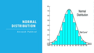
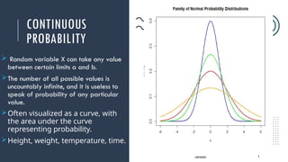
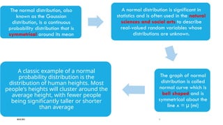
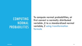
The normal distribution, also called the Gaussian distribution, is one of the most important probability distributions in statistics. It describes how data values are distributed in many natural and social phenomena.Many real-world variables (e.g., height, test scores, measurement errors) follow this distribution. Central Limit Theorem: The sum (or average) of many independent random variables tends to be normally distributed, even if the original variables themselves are not

1. NORMAL
DISTRIBUTION
A n we s h Po k h r e l

2. AGENDA
2
•Continuous Probability
Distribution
•Difference between
discrete and continuous
variable
•Normal Distribution
•Characteristics
•Example
•Z transformation formula
•Example

3. CONTINUOUS
PROBABILITY
 Random variable X can take any value
between certain limits a and b.
The number of all possible values is
uncountably infinite, and it is useless to
speak of probability of any particular
value.
Often visualized as a curve, with
the area under the curve
representing probability.
Height, weight, temperature, time.
CONTINUOUS 3

5. 08/02/2025 PDF 5
Described by a probability density function (PDF), which
shows the likelihood of a variable assuming specific values.

6. NORMAL
DISTRIBUTION
Johann Friedrich
Carl Gauss the
greatest German
mathematician in
1809 introduce
normal distribution.
Therefore, it is also
called as Gaussian
Distribution.
Johann Fredrich
Carl Gauss first
described normal
distribution when
he measured
errors in
astronomy.

7. 08/02/2025 7
The normal distribution, also
known as the Gaussian
distribution, is a continuous
probability distribution that is
symmetrical around its mean
A normal distribution is significant in
statistics and is often used in the natural
sciences and social arts to describe
real-valued random variables whose
distributions are unknown.
The graph of normal
distribution is called
normal curve which is
bell shaped and is
symmetrical about the
line x = µ (mi)
A classic example of a normal
probability distribution is the
distribution of human heights. Most
people's heights will cluster around the
average height, with fewer people
being significantly taller or shorter
than average

8. CHARACTERISTICS
08/02/2025
8
In a normal distribution, the mean, median and
mode are equal.(i.e., Mean = Median= Mode).
The total area under the curve should be equal to
1.
Mean = µ, Standard Deviation = (
σ sigma),
Skewness = 0 and kurtosis = 3
The normally distributed curve should be
symmetric at the center.
There should be exactly half of the values are to
the right of the center and exactly half of the
values are to the left of the center.

9. 08/02/2025 9
The normal distribution
should be defined by the
mean and standard
deviation.
The normal distribution
curve must have only one
peak. (i.e., Unimodal)
The curve approaches the x-
axis, but it never touches, and
it extends farther away from
the mean

10. 08/02/2025 10

11. 08/02/2025 FORMULA 11
Normal Distribution Formula
The probability density function of
normal or gaussian distribution is given
by;
Where,
•x is the variable
•μ is the mean
•σ is the standard deviation
π is 3.1416
e is 2.71828 approximate.

12. ONE EXAMPLE
08/02/2025 12
Calculate the probability density function of normal distribution using the following data.
x = 3, μ = 4 and σ = 2.
Solution: Given,
variable, x = 3
Mean = 4 and
Standard deviation = 2
By the formula of the probability density of normal distribution, we can write;
Hence, f(3,4,2) = 1.106.

13. NORMAL
DISTRIBUTION
STANDARD
DEVIATION
The standard deviations are used to
subdivide the area under the normal curve.
Each subdivided section defines the
percentage of data, which falls into the
specific region of a graph.
Using 1 standard deviation, the Empirical Rule
states that,
Thus, the empirical rule is also called the
68 – 95 – 99.7 rule
13

14. 08/02/2025 14
Approximately 95% of the data falls within two standard deviations of
the mean. (i.e., Between Mean- two Standard Deviation and Mean + two
standard deviations)
Approximately 99.7% of the data fall within three standard deviations
of the mean. (i.e., Between Mean- three Standard Deviation and Mean +
three standard deviations)
Approximately 68% of the data falls within one standard deviation of
the mean. (i.e., Between Mean- one Standard Deviation and Mean + one
standard deviation)

15. 15
The empirical rule is called the 68 – 95 – 99.7 rule

16. COMPUTING
NORMAL
PROBABILITIES
To compute normal probabilities, at
first convert a normally distributed
variable ,X to a standardized normal
variable, Z using transformation
formula
08/02/2025 16

17. Z TRANSFORMATIVE
FORMULA
08/02/2025 17
𝑋 − 𝜇
𝜎
Z =
Finding X value
Z =
Or, Z
Or, X = µ +Z

18. 08/02/2025 PRESENTATION TITLE 18

19. 19
For some computers, the time period between charges of the battery is normally distributed
with a mean of 50 hours and a standard deviation of 15 hours. Mr. A has one of these
computers and needs to know the probability that the time period will be between 50 and 70
hours.
Solution: Let x be the random variable that represents the time period.
Given
Mean, μ= 50
and standard deviation, σ = 15
To find: Probability that x is between 50 and 70 or P( 50< x < 70)
By using the transformation equation, we know;
z = (X – μ) / σ
For x = 50 , z = (50 – 50) / 15 = 0
For x = 70 , z = (70 – 50) / 15 = 1.33
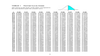
P( 50< x < 70) = P( 0< z < 1.33) = [area to the left of z = 1.33] – [area to the left of z = 0]
From the table we get the value, such as;
P( 0< z < 1.33) = 0.9082 – 0.5 = 0.4082
The probability that Rohan’s computer has a time period between 50 and 70 hours is equal to
0.4082.

20. A PICTURE IS
WORTH THAN
THOUSAND
WORDS
08/02/2025 THANKS 20
Thank You !