Downloaded 49 times
![10.2 WAVES IN GENERAL 411
ing of EM waves. The reader who is conversant with the concept of waves may skip
Section 10.2. Power considerations, reflection, and transmission between two different
media will be discussed later in the chapter.
10.2 WAVES IN GENERAL
A clear understanding of EM wave propagation depends on a grasp of what waves are in
general.
A wave is a function of both space and time.
Wave motion occurs when a disturbance at point A, at time to, is related to what happens at
point B, at time t > t0. A wave equation, as exemplified by eqs. (9.51) and (9.52), is a
partial differential equation of the second order. In one dimension, a scalar wave equation
takes the form of
d2E 2 d2E
r- - U r- = 0 (10.1)
dt2 dz2
where u is the wave velocity. Equation (10.1) is a special case of eq. (9.51) in which the
medium is source free (pv, = 0, J = 0). It can be solved by following procedure, similar to
that in Example 6.5. Its solutions are of the form
E =f(z~ ut) (10.2a)
E+ = g(z + ut) (10.2b)
or
E=f(z- ut) + g(z + ut) (10.2c)
where / and g denote any function of z — ut and z + ut, respectively. Examples of such
functions include z ± ut, sin k(z ± ut), cos k(z ± ut), and eJk(-z±u' where k is a constant. It
can easily be shown that these functions all satisfy eq. (10.1).
If we particularly assume harmonic (or sinusoidal) time dependence eJ0", eq. (10.1)
becomes
d2E,
S = 0 (10.3)
where /3 = u/u and Es is the phasor form of E. The solution to eq. (10.3) is similar to
Case 3 of Example 6.5 [see eq. (6.5.12)]. With the time factor inserted, the possible solu-
tions to eq. (10.3) are
+ (10.4a)
E =
(10.4b)](https://image.slidesharecdn.com/copyofchapter10-100926044334-phpapp02/85/Copy-of-chapter-10-2-320.jpg)
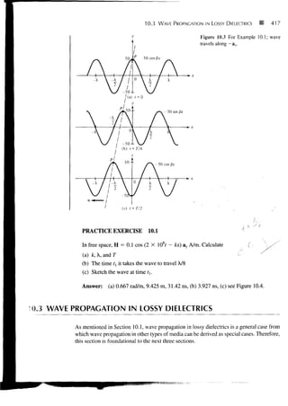
![10.3 WAVE PROPAGATION IN LOSSY DIELECTRICS • 421
with
(10.33)
where 0 < 6V < 45°. Substituting eqs. (10.31) and (10.32) into eq. (10.30) gives
or
H = ~ e~az cos(co? - pz- 0,) (10.34)
Notice from eqs. (10.29) and (10.34) that as the wave propagates along az, it decreases or
attenuates in amplitude by a factor e~az, and hence a is known as the attenuation constant
or attenuation factor of the medium. It is a measure of the spatial rate of decay of the wave
in the medium, measured in nepers per meter (Np/m) or in decibels per meter (dB/m). An
attenuation of 1 neper denotes a reduction to e~l of the original value whereas an increase
of 1 neper indicates an increase by a factor of e. Hence, for voltages
1 Np = 20 log10 e = 8.686 dB (10.35)
From eq. (10.23), we notice that if a = 0, as is the case for a lossless medium and free
space, a = 0 and the wave is not attenuated as it propagates. The quantity (3 is a measure
of the phase shift per length and is called the phase constant or wave number. In terms of
/?, the wave velocity u and wavelength X are, respectively, given by [see eqs. (10.7b) and
(10.8)]
CO 2x (10.36)
X =
0
We also notice from eqs. (10.29) and (10.34) that E and H are out of phase by 0, at any
instant of time due to the complex intrinsic impedance of the medium. Thus at any time, E
leads H (or H lags E) by 6V. Finally, we notice that the ratio of the magnitude of the con-
duction current density J to that of the displacement current density Jd in a lossy medium
is
= tan I
IX*
0)8
or
tan 6 = — (10.37)
coe](https://image.slidesharecdn.com/copyofchapter10-100926044334-phpapp02/85/Copy-of-chapter-10-12-320.jpg)
![10.6 PLANE WAVES IN G O O D CONDUCTORS 431
where Hj = -0.1 cos (uf - z) ax and H 2 = 0.5 sin (wt - z) ay and the corresponding
electric field
E = E, + E 7
where Ej = Elo cos (cof - z) a £i and E 2 = E2o sin (cof - z) aEi. Notice that although H
has components along ax and ay, it has no component along the direction of propagation; it
is therefore a TEM wave.
ForEb
afi] = -(a* X aHl) = - ( a , X - a x ) = a,
Eo = V Hlo = 60TT (0.1) = 6TT
Hence
= 6x cos {bit — z) av
ForE,
aEl = ~{akx aH) = -{az X ay) = ax
E2o = V H2o = 60TT (0.5) = 30x
Hence
E 2 = 30TT sin {wt - z)ax
Adding E) and E 2 gives E; that is,
E = 94.25 sin (1.5 X 10⁸f - z) ax + 18.85 cos (1.5 X 10⁸? - z) ay V/m
Method 2: We may apply Maxwell's equations directly.
1
V X H = iE + s •
dt
0
because a = 0. But
JL JL A.
dHy dHx
V X H = dx dy dz
Hx(z) Hv(z) 0
= H2o cos {bit - z) ax + Hlo sin (wf - z)ay
where Hlo = -0.1 and// 2o = 0.5. Hence
if W W
E=- V x H ( i ( = — sin (wf - z) a, cos (cor - z) a,,
e J eco eco '
= 94.25 sin(cor - z)ax+ 18.85 cos(wf - z) a, V/m
as expected.](https://image.slidesharecdn.com/copyofchapter10-100926044334-phpapp02/85/Copy-of-chapter-10-22-320.jpg)
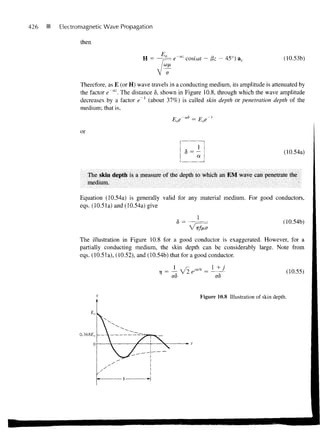
![434 Electromagnetic Wave Propagation
The constant B must be zero because Jsx is finite as z~> °°. But in a good conductor,
a ^> we so that a = /3 = 1/5. Hence
(1 + j)
7 = a + jf3 = a(l + j) =
and
= Ae~*
or
where Jsx (0) is the current density on the conductor surface.
PRACTICE EXERCISE 10.5
Due to the current density of Example 10.5, find the magnitude of the total current
through a strip of the conductor of infinite depth along z and width w along y.
Answer:
V~2
For the copper coaxial cable of Figure 7.12, let a = 2 mm, b = 6 mm, and t = 1 mm. Cal-
EXAMPLE 10.6
culate the resistance of 2 m length of the cable at dc and at 100 MHz.
Solution:
Let
R = Ro + Ri
where Ro and Rt are the resistances of the inner and outer conductors.
Atdc,
= 2.744 mfi
aira2 5.8 X 10 7 TT[2 X 10~ 3 ] 2
/?„ = — =
aS oir[[b + t]2 - b2] air[t2 + 2bt
2
~ 5.8 X 10⁷TT [1 + 12] X 10" 6
= 0.8429 mO
Hence Rdc = 2.744 + 0.8429 = 3.587 mfi](https://image.slidesharecdn.com/copyofchapter10-100926044334-phpapp02/85/Copy-of-chapter-10-25-320.jpg)
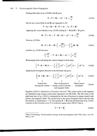
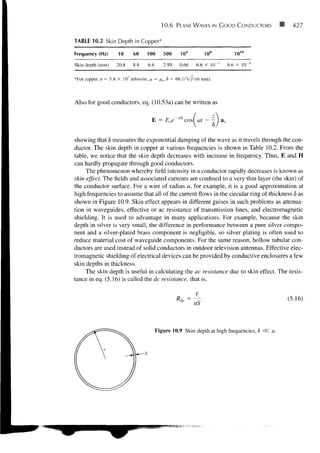
![438 Electromagnetic Wave Propagation
and
E2
<3>(z, 0 = 7-7 e~2az cos (cot - fiz) cos (cot - Hz - 0J a,
(10.66)
M
2az
e [cos 6 + cos (2cot - 2/3z - 6 )] a-
since cos A cos B = — [cos (A — 5) + cos (A + B)]. To determine the time-average
Poynting vector 2?ave(z) (in W/m2), which is of more practical value than the instantaneous
Poynting vector 2P(z, t), we integrate eq. (10.66) over the period T = 2ir/u>; that is,
dt (10.67)
It can be shown (see Prob. 10.28) that this is equivalent to
(10.68)
By substituting eq. (10.66) into eq. (10.67), we obtain
(10.69)
J
The total time-average power crossing a given surface S is given by
p — Of, (10.70)
We should note the difference between 2?, S?ave, and P ave . SP(*> y. z. 0 i s m e Poynting
vector in watts/meter and is time varying. 2PaVe0c, y, z) also in watts/meter is the time
average of the Poynting vector S?; it is a vector but is time invariant. P ave is a total time-
average power through a surface in watts; it is a scalar.
In a nonmagnetic medium
EXAMPLE 10.7
E = 4 sin (2TT X 107 - 0.8*) a, V/m](https://image.slidesharecdn.com/copyofchapter10-100926044334-phpapp02/85/Copy-of-chapter-10-29-320.jpg)
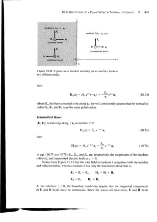
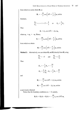
![10.8 REFLECTION OF A PLANE WAVE AT NORMAL INCIDENCE 443
travel; it consists of two traveling waves (E, and Er) of equal amplitudes but in opposite di-
rections. Combining eqs. (10.71) and (10.73) gives the standing wave in medium 1 as
yz
Els = E,,. + E r a = (Eioe ' + Eroey'z) a x (10.84)
But
Hence,
E , , = -Eio(ei0'z - e--^z) a x
or
(10.85)
Thus
E, = Re (E]seM)
or
E{ = 2Eio sin (3^ sin ut ax (10.86)
By taking similar steps, it can be shown that the magnetic field component of the wave is
2Eio
Hi = cos p,z cos u>t a v (10.87)
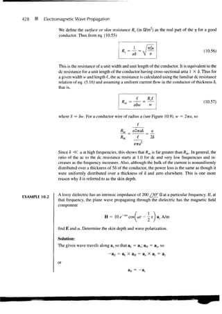
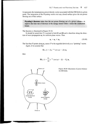
A sketch of the standing wave in eq. (10.86) is presented in Figure 10.12 for t = 0, 778,
774, 3778, 772, and so on, where T = 2TT/W. From the figure, we notice that the wave does
not travel but oscillates.
When media 1 and 2 are both lossless we have another special case (a{ = 0 = a2). In
this case, ^ and rj2 a r e r e a l a n d so are F and T. Let us consider the following cases:
CASE A.
If r/2 > Jji, F > 0. Again there is a standing wave in medium 1 but there is also a transmit-
ted wave in medium 2. However, the incident and reflected waves have amplitudes that are
not equal in magnitude. It can be shown that the maximum values of |EX j occur at
^l^-inax = WE
or
mr
n = 0, 1, 2, . . . (10.:
2 '](https://image.slidesharecdn.com/copyofchapter10-100926044334-phpapp02/85/Copy-of-chapter-10-34-320.jpg)
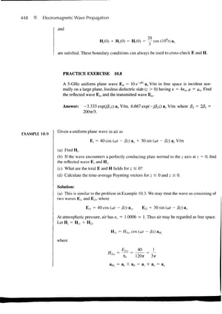
![444 Electromagnetic Wave Propagation
• JX
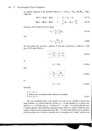
Figure 10.12 Standing waves E = 2Eio sin /3,z sin oit &x; curves
0, 1, 2, 3, 4, . . . are, respectively, at times t = 0, 778, TIA, 37/8, 772,. . .;
X = 2x7/3,.
and the minimum values of |E t | occur at
-/3,z min = (2« + 1)
or
+ (2w + 1)
w — u, l, z, (10.89)
2/3,
CASE B.
If r/2 < r/!, T < 0. For this case, the locations of |Ej| maximum are given by eq. (10.89)
whereas those of |EX | minimum are given by eq. (10.88). All these are illustrated in Figure
10.13. Note that
1. |H] j minimum occurs whenever there is |Ei | maximum and vice versa.
2. The transmitted wave (not shown in Figure 10.13) in medium 2 is a purely travel-
ing wave and consequently there are no maxima or minima in this region.
The ratio of |Ei | max to |E, | min (or |Hj | max to |Hj | min ) is called the standing-wave ratio
s; that is,
Mi l+ r |
s= (10.90)
IH, l- r](https://image.slidesharecdn.com/copyofchapter10-100926044334-phpapp02/85/Copy-of-chapter-10-35-320.jpg)
![450 Electromagnetic Wave Propagation
(c) The total fields in air
E, = E, + E r and H, = H, + H r
can be shown to be standing wave. The total fields in the conductor are
E 2 = Er = 0, H2 = H, = 0.
(d) For z < 0,
™ _ IE,/ 1 2 2
= T — [Eioaz - Emaz]
2»?
1 2 2
[(402 + 302)az - (402 + 302)
)aJ
240TT
= 0
For z > 0 ,
op —
|E 2
= ^ a 7 = 0
2rj 2
because the whole incident power is reflected.
PRACTICE EXERCISE 10.9
The plane wave E = 50 sin (o)t — 5x) ay V/m in a lossless medium (n = 4/*o,
e = so) encounters a lossy medium (fi = no, e = 4eo, < = 0.1 mhos/m) normal to
r
the x-axis at x = 0. Find
(a) F, T, and s
(b) E r andH r
(c) E r andH,
(d) The time-average Poynting vectors in both regions
Answer: (a) 0.8186 /171.1°, 0.2295 /33.56°, 10.025, (b) 40.93 sin (ait + 5x +
171.9°) ay V/m, -54.3 sin (at + 5x + 171.9° az mA/m,
(c) 11.47 e~6-UZI*sin (cor -7.826x + 33.56°) ay V/m, 120.2 e-6.02U sin
M - 7.826x - 4.01°) a, mA/m, (d) 0.5469 &x W/m2, 0.5469 exp
(-12.04x)a x W/m 2 .](https://image.slidesharecdn.com/copyofchapter10-100926044334-phpapp02/85/Copy-of-chapter-10-41-320.jpg)
![10.9 REFLECTION OF A PLANE WAVE AT OBLIQUE INCIDENCE 451
10.9 REFLECTION OF A PLANE WAVE
T OBLIQUE INCIDENCE
We now consider a more general situation than that in Section 10.8. To simplify the analy-
sis, we will assume that we are dealing with lossless media. (We may extend our analysis
to that of lossy media by merely replacing e by sc.) It can be shown (see Problems 10.14
and 10.15) that a uniform plane wave takes the general form of
E(r, t) = E o cos(k • r - cof)
(10.93)
= Re [EoeKkr-wt)]
where r = xax + yay + zaz is the radius or position vector and k = kxax + kyay + kzaz is
the wave number vector or the propagation vector; k is always in the direction of wave
propagation. The magnitude of k is related to a according to the dispersion relation
>
k2 = k2x k, k] = (10.94)
Thus, for lossless media, k is essentially the same as (3 in the previous sections. With the
general form of E as in eq. (10.93), Maxwell's equations reduce to
k XE = (10.95a)
k XH = - (10.95b)
k H = 0 (10.95c)
k-E = 0 (10.95d)
showing that (i) E, H, and k are mutually orthogonal, and (ii) E and H lie on the plane
k • r = kjc + kyy + kzz = constant
From eq. (10.95a), the H field corresponding to the E field in eq. (10.93) is
(10.96)
77
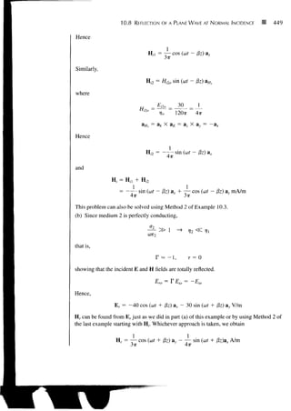
Having expressed E and H in the general form, we can now consider the oblique inci-
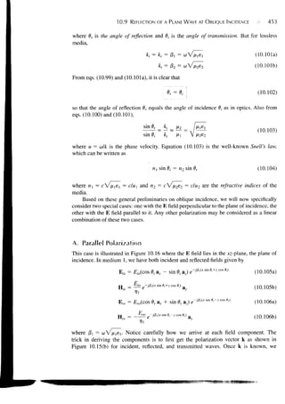
dence of a uniform plane wave at a plane boundary as illustrated in Figure 10.15(a). The
plane denned by the propagation vector k and a unit normal vector an to the boundary is
called the plane of incidence. The angle 0, between k and an is the angle of incidence.
Again, both the incident and the reflected waves are in medium 1 while the transmit-
ted (or refracted wave) is in medium 2. Let
E,- = Eio cos (kixx + kiyy + kizz - us-t) (10.97a)
E r = E ro cos (krxx + kny + krzz - cV) (10.97b)
E, = E ro cos (ktxx + ktyy + ktzz - u,t) (10.97c)](https://image.slidesharecdn.com/copyofchapter10-100926044334-phpapp02/85/Copy-of-chapter-10-42-320.jpg)
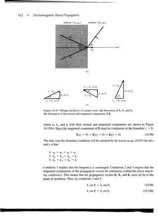
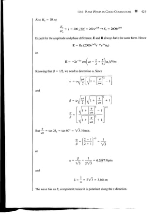
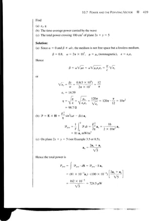
![454 Electromagnetic Wave Propagation
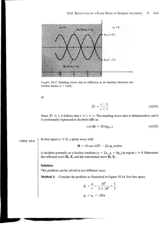
Figure 10.16 Oblique incidence with E par-
allel to the plane of incidence.
medium 1 z- 0 medium 2
define E s such that V • E.v = 0 or k • E s = 0 and then H s is obtained from H s =
k E
— X E , = a* X - .
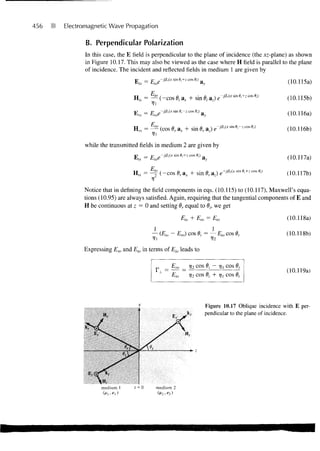
The transmitted fields exist in medium 2 and are given by
E, s = £ M (cos 0, a x - sin 0, a,) e->&usine,+Jcose,) (10.107a)
H ( i = - ^ e ^ « x s m fl, + z cos 0,)
(10.107b)
where f32 = o V /u2e2. Should our assumption about the relative directions in eqs. (10.105)
>
to (10.107) be wrong, the final result will show us by means of its sign.
Requiring that dr = dj and that the tangential components of E and H be continuous at
the boundary z — 0, we obtain
(Ei0 + Ero) cos 0,- = E,o cos 0t (10.108a)
— (£,„ - Em) = — Eto (10.108b)
Expressing Em and Eta in terms of Eio, we obtain
_ Ero. _ 11 COS 0, ~ •>?! COS 0,-
(10.109a)
£,o 7j2 cos 0, + rjj cos 0 ;
or
(10.109b)
and
£to _ 2r;2 cos 0,
(10.110a)
Eio 7]2 cos 0, + r | cos 0,](https://image.slidesharecdn.com/copyofchapter10-100926044334-phpapp02/85/Copy-of-chapter-10-45-320.jpg)
![10.9 REFLECTION OF A PLANE WAVE AT OBLIQUE INCIDENCE 457
or
ro ^ J_ io (10.119b)
and
(10.120a)
Eio ri2 cos 6,• + vl cos 9,
or
Eto - (10.120b)
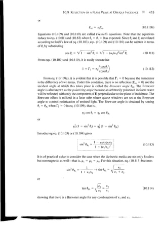
which are the Fresnel's equations for perpendicular polarization. From eqs. (10.119) and
(10.120), it is easy to show that
1 + r ± = TL (10.121)
which is similar to eq. (10.83) for normal incidence. Also, when 9/ = 9, = 0, eqs. (10.119)
and (10.120) become eqs. (10.81) and (10.82) as they should.
For no reflection, TL = 0 (or Er = 0). This is the same as the case of total transmis-
sion (TX = 1). By replacing 0, with the corresponding Brewster angle 9B±, we obtain
t2 cos 9B± = ry,cos 9,
or
- sin20()
Incorporating eq. (10.104) yields
AM 6 2
sin2 9Bx = (10.122)
Note that for nonmagnetic media (ft, = A*2 = AO, sin2 0B± ""* °° i n eq- (10.122), so 9BL
does not exist because the sine of an angle is never greater than unity. Also if /x, + JX2 and
6] = e2, eq. (10.122) reduces to
sin 1
or
(10.123)
Although this situation is theoretically possible, it is rare in practice.](https://image.slidesharecdn.com/copyofchapter10-100926044334-phpapp02/85/Copy-of-chapter-10-48-320.jpg)
![460 Electromagnetic Wave Propagation
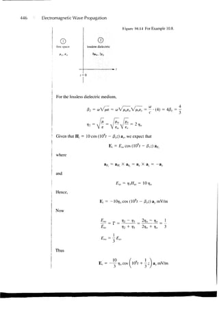
j (c) An easy way to find E r is to use eq. (10.116a) because we have noticed that this
1 problem is similar to that considered in Section 10.9(b). Suppose we are not aware of this.
I Let
j Er = Ero cos (cor - kr • r) ay
> which is similar to form to the given E,. The unit vector ay is chosen in view of the fact that
i the tangential component of E must be continuous at the interface. From Figure 10.18,
k r = krx ax — krz az
where
• krx = kr sin 9n krz = kr cos 6r
But 6r = Oj and kr = k}• = 5 because both kr and k{ are in the same medium. Hence,
kr = Aax - 3a z
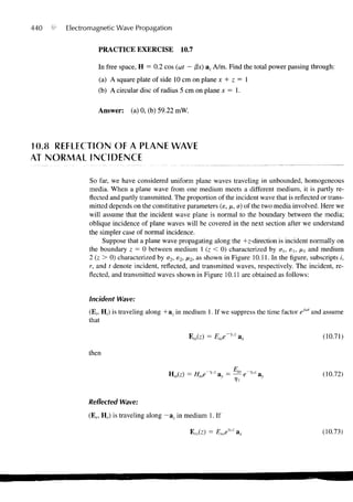
To find Em, we need 6t. From Snell's law
sin 6, = — sin 0, = sin 8'i
n2
sin 53.13°
2.5
or
6, = 30.39°
Eio
7]2 COS 0; - IJi COS 0,
cos rj! cos 6t
Figure 10.IS Propagation vectors of
ExamplelO.il.](https://image.slidesharecdn.com/copyofchapter10-100926044334-phpapp02/85/Copy-of-chapter-10-51-320.jpg)
![10.9 REFLECTION OF A PLANE WAVE AT OBLIQUE INCIDENCE 461
377
where rjl = rjo = 377, n]2 = = 238.4
238.4 cos 35.13° - 377 cos 30.39°
1
~~ 238.4 cos 53.13° + 377 cos 30.39° ~
Hence,
Em = T±Eio = -0.389(8) = -3.112
and
E, = -3.112 cos (15 X 108f - Ax + 3z)a y V/m
(d) Similarly, let the transmitted electric field be
E, = Eto cos (ut - k, • r) ay
where
W
1
k, = j32 = w V
c
_ 15 X 10 8
3 X 10⁸
From Figure 10.18,
ktx = k, sin 6, = 4
kR = ktcos6, = 6.819
or
k, = 4ax + 6.819 az
Notice that kix = krx = ktx as expected.
_Ew__ 2 7]2 COS dj
Eio i)2 c o s dj + 7)] c o s 6,
2 X 238.4 cos 53.13°
~ 238.4 cos 53.13° + 377 cos 30.39°
= 0.611
The same result could be obtained from the relation T±= + I . Hence,
Eto = TLEio = 0.611 X 8 = 4.888
Ef = 4.888 cos (15 X 108r -Ax- 6.819z) ay](https://image.slidesharecdn.com/copyofchapter10-100926044334-phpapp02/85/Copy-of-chapter-10-52-320.jpg)
![SUMMARY 463
where a = attenuation constant, j3 = phase constant, 7 = |r/|/fln = intrinsic imped-
7
ance of the medium. The reciprocal of a is the skin depth (5 = I/a). The relationship
between /3, w, and X as stated above remain valid for EM waves.
3. Wave propagation in other types of media can be derived from that for lossy media as
special cases. For free space, set a = 0, e = sQ, fi = /xo; for lossless dielectric media,
set a = 0, e = e o s r , and n = jxofxr and for good conductors, set a — °°, e = ea,
H = fio, or a/we — 0.
>
4. A medium is classified as lossy dielectric, lossless dielectric or good conductor depend-
ing on its loss tangent given by
Js a
tan 6 =
h, coe
where ec = e' - je" is the complex permittivity of the medium. For lossless dielectrics
tan0 ^C 1, for good conductors tan d ^J> 1, and for lossy dielectrics tan 6 is of the
order of unity.
5. In a good conductor, the fields tend to concentrate within the initial distance 6 from the
conductor surface. This phenomenon is called skin effect. For a conductor of width w
and length i, the effective or ac resistance is
awd
where < is the skin depth.
5
6. The Poynting vector, 9 is the power-flow vector whose direction is the same as the di-
rection of wave propagation and magnitude the same as the amount of power flowing
through a unit area normal to its direction.
f = EXH, 9>ave = 1/2 Re (E, X H*)
7. If a plane wave is incident normally from medium 1 to medium 2, the reflection coeffi-
cient F and transmission coefficient T are given by
12 = i^= 1 + r
Eio V2 + V
The standing wave ratio, s, is defined as
s=
8. For oblique incidence from lossless medium 1 to lossless medium 2, we have the
Fresnel coefficients as
rj2cos 6, - r] | cos 0, 2?j2 cos 6j
r/2 cos 6, + rjt cos 0/ II = 1)2 COS d + Tfj] COS dj
t](https://image.slidesharecdn.com/copyofchapter10-100926044334-phpapp02/85/Copy-of-chapter-10-54-320.jpg)
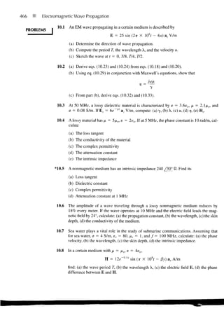
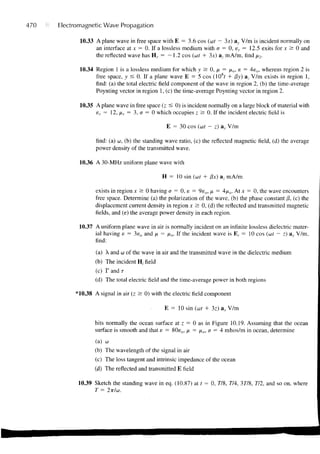
![PROBLEMS 471
Figure 10.19 For Problem 10.38.
H©—»-
ocean
S = 80£ o , |U. = flo, (T = 4
10.40 A uniform plane wave is incident at an angle 0, = 45° on a pair of dielectric slabs joined
together as shown in Figure 10.20. Determine the angles of transmission 0t] and 6,2 in the
slabs.
10.41 Show that the field
E.v = 20 sin (kj) cos (kyy) az
where k2x + k = aj2/ioeo, can be represented as the superposition of four propagating
plane waves. Find the corresponding H,.
10.42 Show that for nonmagnetic dielectric media, the reflection and transmission coefficients
for oblique incidence become
tan (0r~ »,) 2 cos 0; sin 0,
tan (0,4- sin (0, 4- 0;) cos (0, - 0,)
sin (0,- 2 cos 6i sin 6,
r, =-sin (fit + 0,)' sin (0, 4- 0,)
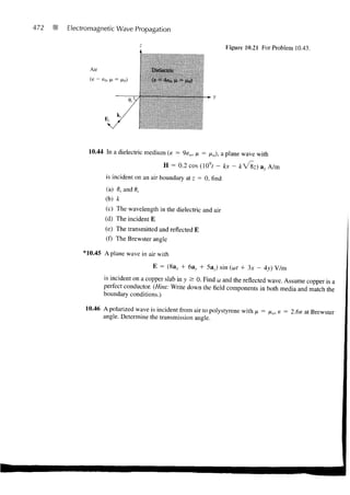
*10.43 A parallel-polarized wave in air with
E = (8a,. - 6a,) sin (cot - Ay - 3z) V/m
impinges a dielectric half-space as shown in Figure 10.21. Find: (a) the incidence angle
0,, (b) the time average in air (/t = pt0, e = e 0 ), (c) the reflected and transmitted E
fields.
Figure 10.2(1 For Problem 10.40.
free space free space](https://image.slidesharecdn.com/copyofchapter10-100926044334-phpapp02/85/Copy-of-chapter-10-62-320.jpg)

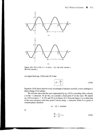
1) This chapter discusses electromagnetic wave propagation based on Maxwell's equations. It will derive wave motion in free space, lossless dielectrics, lossy dielectrics, and good conductors. 2) A wave is a function of both space and time that transports energy or information from one point to another. Electromagnetic waves include radio waves, light, and more. 3) Key wave characteristics include amplitude, wavelength, frequency, period, phase, and velocity. The velocity is the frequency multiplied by the wavelength based on a fixed relationship between them.


![[Solutions manual] elements of electromagnetics BY sadiku - 3rd](https://cdn.slidesharecdn.com/ss_thumbnails/solutionsmanualelementsofelectromagnetics-sadiku-3rd-150605143138-lva1-app6891-thumbnail.jpg?width=640&height=640&fit=bounds)


![[Oficial] solution book elements of electromagnetic 3ed sadiku](https://cdn.slidesharecdn.com/ss_thumbnails/oficialsolutionbook-elementsofelectromagnetic3edsadiku-150423114727-conversion-gate02-thumbnail.jpg?width=640&height=640&fit=bounds)


![[Vvedensky d.] group_theory,_problems_and_solution(book_fi.org)](https://cdn.slidesharecdn.com/ss_thumbnails/vvedenskyd-grouptheoryproblemsandsolutionbookfi-org-130405071812-phpapp02-thumbnail.jpg?width=640&height=640&fit=bounds)