ch09.pdf

8.14. Problems 361
improving liquid crystal displays, and other products, such as various optoelectronic
components, cosmetics, and ”hot” and ”cold” mirrors for architectural and automotive
windows.
8.14 Problems
8.1 Prove the reflectance and transmittance formulas (8.4.6) in FTIR.
8.2 Computer Experiment—FTIR. Reproduce the results and graphs of Figures 8.4.3–8.4.5.
8.3 Computer Experiment—Surface Plasmon Resonance. Reproduce the results and graphs of
Figures 8.5.3–8.5.7.
8.4 Working with the electric and magnetic fields across an negative-index slab given by Eqs. (8.6.1)
and (8.6.2), derive the reflection and transmission responses of the slab given in (8.6.8).
8.5 Computer Experiment—Perfect Lens. Study the sensitivity of the perfect lens property to the
deviations from the ideal values of = −0 and μ = −μ0, and to the presence of losses by
reproducing the results and graphs of Figures 8.6.3 and 8.6.4. You will need to implement
the computational algorithm listed on page 329.
8.6 Computer Experiment—Antireflection Coatings. Reproduce the results and graphs of Figures
8.7.1–8.7.3.
8.7 Computer Experiment—Omnidirectional Dielectric Mirrors. Reproduce the results and graphs
of Figures 8.8.2–8.8.10.
8.8 Derive the generalized Snel’s laws given in Eq. (8.10.10). Moreover, derive the Brewster angle
expressions given in Eqs. (8.11.4) and (8.11.5).
8.9 Computer Experiment—Brewster angles. Study the variety of possible Brewster angles and
reproduce the results and graphs of Example 8.11.1.
8.10 Computer Experiment—Multilayer Birefringent Structures. Reproduce the results and graphs
of Figures 8.13.1–8.13.2.
9
Waveguides
Waveguides are used to transfer electromagnetic power efficiently from one point in
space to another. Some common guiding structures are shown in the figure below.
These include the typical coaxial cable, the two-wire and mictrostrip transmission lines,
hollow conducting waveguides, and optical fibers.
In practice, the choice of structure is dictated by: (a) the desired operating frequency
band, (b) the amount of power to be transferred, and (c) the amount of transmission
losses that can be tolerated.
Fig. 9.0.1 Typical waveguiding structures.
Coaxial cables are widely used to connect RF components. Their operation is practi-
cal for frequencies below 3 GHz. Above that the losses are too excessive. For example,
the attenuation might be 3 dB per 100 m at 100 MHz, but 10 dB/100 m at 1 GHz, and
50 dB/100 m at 10 GHz. Their power rating is typically of the order of one kilowatt at
100 MHz, but only 200 W at 2 GHz, being limited primarily because of the heating of
the coaxial conductors and of the dielectric between the conductors (dielectric voltage
breakdown is usually a secondary factor.) However, special short-length coaxial cables
do exist that operate in the 40 GHz range.
Another issue is the single-mode operation of the line. At higher frequencies, in order
to prevent higher modes from being launched, the diameters of the coaxial conductors
must be reduced, diminishing the amount of power that can be transmitted.
Two-wire lines are not used at microwave frequencies because they are not shielded
and can radiate. One typical use is for connecting indoor antennas to TV sets. Microstrip
lines are used widely in microwave integrated circuits.

9.1. Longitudinal-Transverse Decompositions 363
Rectangular waveguides are used routinely to transfer large amounts of microwave
power at frequencies greater than 3 GHz. For example at 5 GHz, the transmitted power
might be one megawatt and the attenuation only 4 dB/100 m.
Optical fibers operate at optical and infrared frequencies, allowing a very wide band-
width. Their losses are very low, typically, 0.2 dB/km. The transmitted power is of the
order of milliwatts.
9.1 Longitudinal-Transverse Decompositions
In a waveguiding system, we are looking for solutions of Maxwell’s equations that are
propagating along the guiding direction (the z direction) and are confined in the near
vicinity of the guiding structure. Thus, the electric and magnetic fields are assumed to
have the form:
E(x, y, z, t)= E(x, y)ejωt−jβz
H(x, y, z, t)= H(x, y)ejωt−jβz (9.1.1)
where β is the propagation wavenumber along the guide direction. The corresponding
wavelength, called the guide wavelength, is denoted by λg = 2π/β.
The precise relationship between ω and β depends on the type of waveguiding struc-
ture and the particular propagating mode. Because the fields are confined in the trans-
verse directions (the x, y directions,) they cannot be uniform (except in very simple
structures) and will have a non-trivial dependence on the transverse coordinates x and
y. Next, we derive the equations for the phasor amplitudes E(x, y) and H(x, y).
Because of the preferential role played by the guiding direction z, it proves con-
venient to decompose Maxwell’s equations into components that are longitudinal, that
is, along the z-direction, and components that are transverse, along the x, y directions.
Thus, we decompose:
E(x, y)= x̂ Ex(x, y)+ŷ Ey(x, y)

transverse
+ ẑ Ez(x, y)

longitudinal
≡ ET(x, y)+ẑ Ez(x, y) (9.1.2)
In a similar fashion we may decompose the gradient operator:
∇
∇
∇ = x̂ ∂x + ŷ ∂y

transverse
+ ẑ ∂z = ∇
∇
∇T + ẑ ∂z = ∇
∇
∇T − jβ ẑ (9.1.3)
where we made the replacement ∂z → −jβ because of the assumed z-dependence. In-
troducing these decompositions into the source-free Maxwell’s equations we have:
∇
∇
∇ × E = −jωμH
∇
∇
∇ × H = jωE
∇
∇
∇ · E = 0
∇
∇
∇ · H = 0
⇒
(∇
∇
∇T − jβẑ)×(ET + ẑ Ez)= −jωμ(HT + ẑ Hz)
(∇
∇
∇T − jβẑ)×(HT + ẑ Hz)= jω(ET + ẑ Ez)
(∇
∇
∇T − jβẑ)·(ET + ẑ Ez)= 0
(∇
∇
∇T − jβẑ)·(HT + ẑ Hz)= 0
(9.1.4)
364 9. Waveguides
where , μ denote the permittivities of the medium in which the fields propagate, for
example, the medium between the coaxial conductors in a coaxial cable, or the medium
within the hollow rectangular waveguide. This medium is assumed to be lossless for
now.
We note that ẑ · ẑ = 1, ẑ × ẑ = 0, ẑ · ET = 0, ẑ · ∇
∇
∇TEz = 0 and that ẑ × ET and
ẑ × ∇
∇
∇TEz are transverse while ∇
∇
∇T × ET is longitudinal. Indeed, we have:
ẑ × ET = ẑ × (x̂ Ex + ŷ Ey)= ŷ Ex − x̂ Ey
∇
∇
∇T × ET = (x̂ ∂x + ŷ ∂y)×(x̂ Ex + ŷ Ey)= ẑ(∂xEy − ∂yEx)
Using these properties and equating longitudinal and transverse parts in the two
sides of Eq. (9.1.4), we obtain the equivalent set of Maxwell equations:
∇
∇
∇TEz × ẑ − jβ ẑ × ET = −jωμHT
∇
∇
∇THz × ẑ − jβ ẑ × HT = jωET
∇
∇
∇T × ET + jωμ ẑ Hz = 0
∇
∇
∇T × HT − jω ẑ Ez = 0
∇
∇
∇T · ET − jβEz = 0
∇
∇
∇T · HT − jβHz = 0
(9.1.5)
Depending on whether both, one, or none of the longitudinal components are zero,
we may classify the solutions as transverse electric and magnetic (TEM), transverse elec-
tric (TE), transverse magnetic (TM), or hybrid:
Ez = 0, Hz = 0, TEM modes
Ez = 0, Hz = 0, TE or H modes
Ez = 0, Hz = 0, TM or E modes
Ez = 0, Hz = 0, hybrid or HE or EH modes
In the case of TEM modes, which are the dominant modes in two-conductor trans-
mission lines such as the coaxial cable, the fields are purely transverse and the solution
of Eq. (9.1.5) reduces to an equivalent two-dimensional electrostatic problem. We will
discuss this case later on.
In all other cases, at least one of the longitudinal fields Ez, Hz is non-zero. It is then
possible to express the transverse field components ET, HT in terms of the longitudinal
ones, Ez, Hz.
Forming the cross-product of the second of equations (9.1.5) with ẑ and using the
BAC-CAB vector identity, ẑ × (ẑ × HT)= ẑ(ẑ · HT)−HT(ẑ · ẑ)= −HT, and similarly,
ẑ × (∇
∇
∇THz × ẑ)= ∇
∇
∇THz, we obtain:
∇
∇
∇THz + jβHT = jω ẑ × ET
Thus, the first two of (9.1.5) may be thought of as a linear system of two equations
in the two unknowns ẑ × ET and HT, that is,
β ẑ × ET − ωμHT = jẑ × ∇
∇
∇TEz
ω ẑ × ET − βHT = −j∇
∇
∇THz
(9.1.6)

The solution of this system is:
ẑ × ET = −
jβ
k2
c
ẑ × ∇
∇
∇TEz −
jωμ
k2
c
∇
∇
∇THz
HT = −
jω
k2
c
ẑ × ∇
∇
∇TEz −
jβ
k2
c
∇
∇
∇THz
(9.1.7)
where we defined the so-called cutoff wavenumber kc by:
k2
c = ω2
μ − β2
=
ω2
c2
− β2
= k2
− β2
(cutoff wavenumber) (9.1.8)
The quantity k = ω/c = ω
√
μ is the wavenumber a uniform plane wave would
have in the propagation medium , μ.
Although k2
c stands for the difference ω2
μ − β2
, it turns out that the boundary
conditions for each waveguide type force k2
c to take on certain values, which can be
positive, negative, or zero, and characterize the propagating modes. For example, in a
dielectric waveguide k2
c is positive inside the guide and negative outside it; in a hollow
conducting waveguide k2
c takes on certain quantized positive values; in a TEM line, k2
c
is zero. Some related definitions are the cutoff frequency and the cutoff wavelength
defined as follows:
ωc = ckc , λc =
2π
kc
(cutoff frequency and wavelength) (9.1.9)
We can then express β in terms of ω and ωc, or ω in terms of β and ωc. Taking
the positive square roots of Eq. (9.1.8), we have:
β =
1
c

ω2 − ω2
c =
ω
c

1 −
ω2
c
ω2
and ω =

ω2
c + β2c2 (9.1.10)
Often, Eq. (9.1.10) is expressed in terms of the wavelengths λ = 2π/k = 2πc/ω,
λc = 2π/kc, and λg = 2π/β. It follows from k2
= k2
c + β2
that
1
λ2
=
1
λ2
c
+
1
λ2
g
⇒ λg =
λ

1 −
λ2
λ2
c
(9.1.11)
Note that λ is related to the free-space wavelength λ0 = 2πc0/ω = c0/f by the
refractive index of the dielectric material λ = λ0/n.
It is convenient at this point to introduce the transverse impedances for the TE and
TM modes by the definitions:
ηTE =
ωμ
β
= η
ω
βc
, ηTM =
β
ω
= η
βc
ω
(TE and TM impedances) (9.1.12)
366 9. Waveguides
where the medium impedance is η =

μ/, so that η/c = μ and ηc = 1/. We note the
properties:
ηTEηTM = η2
,
ηTE
ηTM
=
ω2
β2c2
(9.1.13)
Because βc/ω =

1 − ω2
c/ω2, we can write also:
ηTE =
η

1 −
ω2
c
ω2
, ηTM = η

1 −
ω2
c
ω2
(9.1.14)
With these definitions, we may rewrite Eq. (9.1.7) as follows:
ẑ × ET = −
jβ
k2
c

ẑ × ∇
∇
∇TEz + ηTE∇
∇
∇THz

HT = −
jβ
k2
c
1
ηTM
ẑ × ∇
∇
∇TEz + ∇
∇
∇THz

(9.1.15)
Using the result ẑ × (ẑ × ET)= −ET, we solve for ET and HT:
ET = −
jβ
k2
c

∇
∇
∇TEz − ηTE ẑ × ∇
∇
∇THz

HT = −
jβ
k2
c

∇
∇
∇THz +
1
ηTM
ẑ × ∇
∇
∇TEz

(transverse fields) (9.1.16)
An alternative and useful way of writing these equations is to form the following
linear combinations, which are equivalent to Eq. (9.1.6):
HT −
1
ηTM
ẑ × ET =
j
β
∇
∇
∇THz
ET − ηTE HT × ẑ =
j
β
∇
∇
∇TEz
(9.1.17)
So far we only used the first two of Maxwell’s equations (9.1.5) and expressed ET, HT
in terms of Ez, Hz. Using (9.1.16), it is easily shown that the left-hand sides of the
remaining four of Eqs. (9.1.5) take the forms:
∇
∇
∇T × ET + jωμ ẑ Hz =
jωμ
k2
c
ẑ

∇2
THz + k2
cHz

∇
∇
∇T × HT − jω ẑ Ez = −
jω
k2
c
ẑ

∇2
TEz + k2
cEz

∇
∇
∇T · ET − jβEz = −
jβ
k2
c

∇2
TEz + k2
cEz

∇
∇
∇T · HT − jβHz = −
jβ
k2
c

∇2
THz + k2
cHz

where ∇2
T is the two-dimensional Laplacian operator:
∇2
T = ∇
∇
∇T · ∇
∇
∇T = ∂2
x + ∂2
y (9.1.18)
and we used the vectorial identities ∇
∇
∇T × ∇
∇
∇TEz = 0, ∇
∇
∇T × (ẑ × ∇
∇
∇THz)= ẑ ∇2
THz, and
∇
∇
∇T · (ẑ × ∇
∇
∇THz)= 0.
It follows that in order to satisfy all of the last four of Maxwell’s equations (9.1.5), it
is necessary that the longitudinal fields Ez(x, y), Hz(x, y) satisfy the two-dimensional
Helmholtz equations:
∇2
TEz + k2
cEz = 0
∇2
THz + k2
cHz = 0
(Helmholtz equations) (9.1.19)
These equations are to be solved subject to the appropriate boundary conditions for
each waveguide type. Once, the fields Ez, Hz are known, the transverse fields ET, HT are
computed from Eq. (9.1.16), resulting in a complete solution of Maxwell’s equations for
the guiding structure. To get the full x, y, z, t dependence of the propagating fields, the
above solutions must be multiplied by the factor ejωt−jβz
.
The cross-sections of practical waveguiding systems have either cartesian or cylin-
drical symmetry, such as the rectangular waveguide or the coaxial cable. Below, we
summarize the form of the above solutions in the two types of coordinate systems.
Cartesian Coordinates
The cartesian component version of Eqs. (9.1.16) and (9.1.19) is straightforward. Using
the identity ẑ × ∇
∇
∇THz = ŷ ∂xHz − x̂ ∂yHz, we obtain for the longitudinal components:
(∂2
x + ∂2
y)Ez + k2
cEz = 0
(∂2
x + ∂2
y)Hz + k2
cHz = 0
(9.1.20)
Eq. (9.1.16) becomes for the transverse components:
Ex = −
jβ
k2
c

∂xEz + ηTE ∂yHz

Ey = −
jβ
k2
c

∂yEz − ηTE ∂xHz

,
Hx = −
jβ
k2
c

∂xHz −
1
ηTM
∂yEz

Hy = −
jβ
k2
c

∂yHz +
1
ηTM
∂xEz

(9.1.21)
Cylindrical Coordinates
The relationship between cartesian and cylindrical coordinates is shown in Fig. 9.1.1.
From the triangle in the figure, we have x = ρ cos φ and y = ρ sin φ. The transverse
gradient and Laplace operator are in cylindrical coordinates:
∇
∇
∇T = ρ̂
ρ
ρ
∂
∂ρ
+ φ̂
φ
φ
1
ρ
∂
∂φ
, ∇
∇
∇2
T =
1
ρ
∂
∂ρ

ρ
∂
∂ρ

+
1
ρ2
∂2
∂φ2
(9.1.22)
368 9. Waveguides
Fig. 9.1.1 Cylindrical coordinates.
The Helmholtz equations (9.1.19) now read:
1
ρ
∂
∂ρ

ρ
∂Ez
∂ρ

+
1
ρ2
∂2
Ez
∂φ2
+ k2
cEz = 0
1
ρ
∂
∂ρ

ρ
∂Hz
∂ρ

+
1
ρ2
∂2
Hz
∂φ2
+ k2
cHz = 0
(9.1.23)
Noting that ẑ × ρ̂
ρ
ρ = φ̂
φ
φ and ẑ × φ̂
φ
φ = −ρ̂
ρ
ρ, we obtain:
ẑ × ∇
∇
∇THz = φ̂
φ
φ(∂ρHz)−ρ̂
ρ
ρ
1
ρ
(∂φHz)
The decomposition of a transverse vector is ET = ρ̂
ρ
ρ Eρ + φ̂
φ
φ Eφ. The cylindrical
coordinates version of (9.1.16) are:
Eρ = −
jβ
k2
c

∂ρEz − ηTE
1
ρ
∂φHz

Eφ = −
jβ
k2
c
1
ρ
∂φEz + ηTE∂ρHz

,
Hρ = −
jβ
k2
c

∂ρHz +
1
ηTMρ
∂φEz

Hφ = −
jβ
k2
c
1
ρ
∂φHz −
1
ηTM
∂ρEz

(9.1.24)
For either coordinate system, the equations for HT may be obtained from those of
ET by a so-called duality transformation, that is, making the substitutions:
E → H , H → −E , → μ , μ → (duality transformation) (9.1.25)
These imply that η → η−1
and ηTE → η−1
TM. Duality is discussed in greater detail in
Sec. 18.2.
9.2 Power Transfer and Attenuation
With the ﬁeld solutions at hand, one can determine the amount of power transmitted
along the guide, as well as the transmission losses. The total power carried by the ﬁelds
along the guide direction is obtained by integrating the z-component of the Poynting
vector over the cross-sectional area of the guide:

9.2. Power Transfer and Attenuation 369
PT =

S
Pz dS , where Pz =
1
2
Re(E × H∗
)·ẑ (9.2.1)
It is easily verified that only the transverse components of the fields contribute to
the power flow, that is, Pz can be written in the form:
Pz =
1
2
Re(ET × H∗
T)·ẑ (9.2.2)
For waveguides with conducting walls, the transmission losses are due primarily to
ohmic losses in (a) the conductors and (b) the dielectric medium filling the space between
the conductors and in which the fields propagate. In dielectric waveguides, the losses
are due to absorption and scattering by imperfections.
The transmission losses can be quantified by replacing the propagation wavenumber
β by its complex-valued version βc = β − jα, where α is the attenuation constant. The
z-dependence of all the field components is replaced by:
e−jβz
→ e−jβcz
= e−(α+jβ)z
= e−αz
e−jβz
(9.2.3)
The quantity α is the sum of the attenuation constants arising from the various loss
mechanisms. For example, if αd and αc are the attenuations due to the ohmic losses in
the dielectric and in the conducting walls, then
α = αd + αc (9.2.4)
The ohmic losses in the dielectric can be characterized either by its loss tangent,
say tan δ, or by its conductivity σd—the two being related by σd = ω tan δ. More
generally, the effective dielectric constant of the medium may have a negative imaginary
part I that includes both conductive and polarization losses, (ω)= − jI, with
I = tan δ. Then, the corresponding complex-valued wavenumber βc is obtained by
the replacement:
β =

ω2μ − k2
c → βc =

ω2μ(ω)−k2
c
For weakly lossy dielectrics (I ), we may make the approximation:
βc =

ω2μ( − jI)−k2
c =

β2 − jω2μI = β

1 − j
ω2
μI
β2

β − j
ω2
μI
2β
Resulting in the attenuation constant, after setting μ = 1/c2
and βc/ω =

1 − ω2
c/ω2,
αd =
ω2
μI
2β
=
1
2
ω2
μ
β
tan δ =
ω tan δ
2c

1 − ω2
c/ω2
(dielectric losses) (9.2.5)
The conductor losses are more complicated to calculate. In practice, the following
approximate procedure is adequate. First, the fields are determined on the assumption
that the conductors are perfect.
370 9. Waveguides
Second, the magnetic fields on the conductor surfaces are determined and the corre-
sponding induced surface currents are calculated by Js = n̂ × H, where n̂ is the outward
normal to the conductor.
Third, the ohmic losses per unit conductor area are calculated by Eq. (2.8.7). Figure
9.2.1 shows such an infinitesimal conductor area dA = dl dz, where dl is along the
cross-sectional periphery of the conductor. Applying Eq. (2.8.7) to this area, we have:
dPloss
dA
=
dPloss
dldz
=
1
2
Rs|Js|2
(9.2.6)
where Rs is the surface resistance of the conductor given by Eq. (2.8.4),
Rs =

ωμ
2σ
= η

ω
2σ
=
1
σδ
, δ =

2
ωμσ
= skin depth (9.2.7)
Integrating Eq. (9.2.6) around the periphery of the conductor gives the power loss per
unit z-length due to that conductor. Adding similar terms for all the other conductors
gives the total power loss per unit z-length:
P
loss =
dPloss
dz
=

Ca
1
2
Rs|Js|2
dl +

Cb
1
2
Rs|Js|2
dl (9.2.8)
Fig. 9.2.1 Conductor surface absorbs power from the propagating fields.
where Ca and Cb indicate the peripheries of the conductors. Finally, the corresponding
attenuation coefficient is calculated from Eq. (2.6.22):
αc =
P
loss
2PT
(conductor losses) (9.2.9)
Equations (9.2.1)–(9.2.9) provide a systematic methodology by which to calculate the
transmitted power and attenuation losses in waveguides. We will apply it to several
examples later on. Eq. (9.2.9) applies also to the dielectric losses so that in general P
loss
arises from two parts, one due to the dielectric and one due to the conducting walls,
α =
P
loss
2PT
=
P
diel + P
cond
2PT
= αd + αc (attenuation constant) (9.2.10)

9.3. TEM, TE, and TM modes 371
Eq. (9.2.5) for αd can also be derived directly from Eq. (9.2.10) by applying it sepa-
rately to the TE and TM modes. We recall from Eq. (1.9.6) that the losses per unit vol-
ume in a dielectric medium, arising from both a conduction and polarization current,
Jtot = J + jωD, are given by,
dPloss
dV
=
1
2
Re

Jtot · E∗

=
1
2
ωI

E · E∗

Integrating over the cross-sectional area of the guide gives the dielectric loss per unit
waveguide length (i.e., z-length),
P
diel =
1
2
ωI

S
|E|2
dS
Applying this to the TE case, we ﬁnd,
P
diel =
1
2
ωI

S
|E|2
dS =
1
2
ωI

S
|ET|2
dS
PT =

S
1
2
Re(ET × H∗
T)·ẑ dS =
1
2ηTE

S
|ET|2
dS =
β
2ωμ

S
|ET|2
dS
αd =
P
diel
2PT
=
ω2
μI
2β
The TM case is a bit more involved. Using Eq. (9.13.1) from Problem 9.11, we ﬁnd,
after using the result, β2
+ k2
c = ω2
μ,
P
diel =
1
2
ωI

S
|E|2
dS =
1
2
ωI

S

|Ez|2
+ |ET|2

dS
=
1
2
ωI

S

|Ez|2
+
β2
k4
c
|∇
∇
∇TEz|2

dS =
1
2
ωI

1 +
β2
k2
c

S
|Ez|2
dS
PT =
1
2ηTM

S
|ET|2
dS =
ω
2β

S
β2
k4
c
|∇
∇
∇TEz|2
dS =
ωβ
2k2
c

S
|Ez|2
dS
αd =
P
diel
2PT
=
1
2
ωI

1 +
β2
k2
c

ωβ
2k2
c
=
ω2
μI
β
9.3 TEM, TE, and TM modes
The general solution described by Eqs. (9.1.16) and (9.1.19) is a hybrid solution with non-
zero Ez and Hz components. Here, we look at the specialized forms of these equations
in the cases of TEM, TE, and TM modes.
One common property of all three types of modes is that the transverse fields ET, HT
are related to each other in the same way as in the case of uniform plane waves propagat-
ing in the z-direction, that is, they are perpendicular to each other, their cross-product
points in the z-direction, and they satisfy:
372 9. Waveguides
HT =
1
ηT
ẑ × ET (9.3.1)
where ηT is the transverse impedance of the particular mode type, that is, η, ηTE, ηTM
in the TEM, TE, and TM cases.
Because of Eq. (9.3.1), the power flow per unit cross-sectional area described by the
Poynting vector Pz of Eq. (9.2.2) takes the simple form in all three cases:
Pz =
1
2
Re(ET × H∗
T)·ẑ =
1
2ηT
|ET|2
=
1
2
ηT|HT|2
(9.3.2)
TEM modes
In TEM modes, both Ez and Hz vanish, and the fields are fully transverse. One can set
Ez = Hz = 0 in Maxwell equations (9.1.5), or equivalently in (9.1.16), or in (9.1.17).
From any point view, one obtains the condition k2
c = 0, or ω = βc. For example, if
the right-hand sides of Eq. (9.1.17) vanish, the consistency of the system requires that
ηTE = ηTM, which by virtue of Eq. (9.1.13) implies ω = βc. It also implies that ηTE, ηTM
must both be equal to the medium impedance η. Thus, the electric and magnetic fields
satisfy:
HT =
1
η
ẑ × ET (9.3.3)
These are the same as in the case of a uniform plane wave, except here the fields
are not uniform and may have a non-trivial x, y dependence. The electric field ET is
determined from the rest of Maxwell’s equations (9.1.5), which read:
∇
∇
∇T × ET = 0
∇
∇
∇T · ET = 0
(9.3.4)
These are recognized as the field equations of an equivalent two-dimensional elec-
trostatic problem. Once this electrostatic solution is found, ET(x, y), the magnetic field
is constructed from Eq. (9.3.3). The time-varying propagating fields will be given by
Eq. (9.1.1), with ω = βc. (For backward moving fields, replace β by −β.)
We explore this electrostatic point of view further in Sec. 11.1 and discuss the cases
of the coaxial, two-wire, and strip lines. Because of the relationship between ET and HT,
the Poynting vector Pz of Eq. (9.2.2) will be:
Pz =
1
2
Re(ET × H∗
T)·ẑ =
1
2η
|ET|2
=
1
2
η|HT|2
(9.3.5)

9.3. TEM, TE, and TM modes 373
TE modes
TE modes are characterized by the conditions Ez = 0 and Hz = 0. It follows from the
second of Eqs. (9.1.17) that ET is completely determined from HT, that is, ET = ηTEHT×ẑ.
The ﬁeld HT is determined from the second of (9.1.16). Thus, all ﬁeld components
for TE modes are obtained from the equations:
∇2
THz + k2
cHz = 0
HT = −
jβ
k2
c
∇
∇
∇THz
ET = ηTE HT × ẑ
(TE modes) (9.3.6)
The relationship of ET and HT is identical to that of uniform plane waves propagating
in the z-direction, except the wave impedance is replaced by ηTE. The Poynting vector
of Eq. (9.2.2) then takes the form:
Pz =
1
2
Re(ET × H∗
T)·ẑ =
1
2ηTE
|ET|2
=
1
2
ηTE|HT|2
=
1
2
ηTE
β2
k4
c
|∇
∇
∇THz|2
(9.3.7)
The cartesian coordinate version of Eq. (9.3.6) is:
(∂2
x + ∂2
y)Hz + k2
cHz = 0
Hx = −
jβ
k2
c
∂xHz , Hy = −
jβ
k2
c
∂yHz
Ex = ηTE Hy , Ey = −ηTE Hx
(9.3.8)
And, the cylindrical coordinate version:
1
ρ
∂
∂ρ

ρ
∂Hz
∂ρ

+
1
ρ2
∂2
Hz
∂φ2
+ k2
cHz = 0
Hρ = −
jβ
k2
c
∂Hz
∂ρ
, Hφ = −
jβ
k2
c
1
ρ
∂Hz
∂φ
Eρ = ηTE Hφ , Eφ = −ηTE Hρ
(9.3.9)
where we used HT × ẑ = (ρ̂
ρ
ρ Hρ + φ̂
φ
φ Hφ)×ẑ = −φ̂
φ
φ Hρ + ρ̂
ρ
ρ Hφ.
TM modes
TM modes have Hz = 0 and Ez = 0. It follows from the first of Eqs. (9.1.17) that HT is
completely determined from ET, that is, HT = η−1
TMẑ × ET. The field ET is determined
from the first of (9.1.16), so that all field components for TM modes are obtained from
the following equations, which are dual to the TE equations (9.3.6):
374 9. Waveguides
∇2
TEz + k2
cEz = 0
ET = −
jβ
k2
c
∇
∇
∇TEz
HT =
1
ηTM
ẑ × ET
(TM modes) (9.3.10)
Again, the relationship of ET and HT is identical to that of uniform plane waves
propagating in the z-direction, but the wave impedance is now ηTM. The Poynting vector
takes the form:
Pz =
1
2
Re(ET × H∗
T)·ẑ =
1
2ηTM
|ET|2
=
1
2ηTM
β2
k4
c
|∇
∇
∇TEz|2
(9.3.11)
9.4 Rectangular Waveguides
Next, we discuss in detail the case of a rectangular hollow waveguide with conducting
walls, as shown in Fig. 9.4.1. Without loss of generality, we may assume that the lengths
a, b of the inner sides satisfy b ≤ a. The guide is typically filled with air, but any other
dielectric material , μ may be assumed.
Fig. 9.4.1 Rectangular waveguide.
The simplest and dominant propagation mode is the so-called TE10 mode and de-
pends only on the x-coordinate (of the longest side.) Therefore, we begin by looking
for solutions of Eq. (9.3.8) that depend only on x. In this case, the Helmholtz equation
reduces to:
∂2
xHz(x)+k2
cHz(x)= 0
The most general solution is a linear combination of cos kcx and sin kcx. However,
only the former will satisfy the boundary conditions. Therefore, the solution is:
Hz(x)= H0 cos kcx (9.4.1)
where H0 is a (complex-valued) constant. Because there is no y-dependence, it follows
from Eq. (9.3.8) that ∂yHz = 0, and hence Hy = 0 and Ex = 0. It also follows that:
Hx(x)= −
jβ
k2
c
∂xHz = −
jβ
k2
c
(−kc)H0 sin kcx =
jβ
kc
H0 sin kcx ≡ H1 sin kcx

9.4. Rectangular Waveguides 375
Then, the corresponding electric field will be:
Ey(x)= −ηTE Hx(x)= −ηTE
jβ
kc
H0 sin kcx ≡ E0 sin kcx
where we defined the constants:
H1 =
jβ
kc
H0
E0 = −ηTE H1 = −ηTE
jβ
kc
H0 = −jη
ω
ωc
H0
(9.4.2)
where we used ηTE = ηω/βc. In summary, the non-zero field components are:
Hz(x)= H0 cos kcx
Hx(x)= H1 sin kcx
Ey(x)= E0 sin kcx
⇒
Hz(x, y, z, t)= H0 cos kcx ejωt−jβz
Hx(x, y, z, t)= H1 sin kcx ejωt−jβz
Ey(x, y, z, t)= E0 sin kcx ejωt−jβz
(9.4.3)
Assuming perfectly conducting walls, the boundary conditions require that there be
no tangential electric field at any of the wall sides. Because the electric field is in the
y-direction, it is normal to the top and bottom sides. But, it is parallel to the left and
right sides. On the left side, x = 0, Ey(x) vanishes because sin kcx does. On the right
side, x = a, the boundary condition requires:
Ey(a)= E0 sin kca = 0 ⇒ sin kca = 0
This requires that kca be an integral multiple of π:
kca = nπ ⇒ kc =
nπ
a
(9.4.4)
These are the so-called TEn0 modes. The corresponding cutoff frequency ωc = ckc,
fc = ωc/2π, and wavelength λc = 2π/kc = c/fc are:
ωc =
cnπ
a
, fc =
cn
2a
, λc =
2a
n
(TEn0 modes) (9.4.5)
The dominant mode is the one with the lowest cutoff frequency or the longest cutoff
wavelength, that is, the mode TE10 having n = 1. It has:
kc =
π
a
, ωc =
cπ
a
, fc =
c
2a
, λc = 2a (TE10 mode) (9.4.6)
Fig. 9.4.2 depicts the electric field Ey(x)= E0 sin kcx = E0 sin(πx/a) of this mode
as a function of x.
376 9. Waveguides
Fig. 9.4.2 Electric field inside a rectangular waveguide.
9.5 Higher TE and TM modes
To construct higher modes, we look for solutions of the Helmholtz equation that are
factorable in their x and y dependence:
Hz(x, y)= F(x)G(y)
Then, Eq. (9.3.8) becomes:
F
(x)G(y)+F(x)G
(y)+k2
cF(x)G(y)= 0 ⇒
F
(x)
F(x)
+
G
(y)
G(y)
+ k2
c = 0 (9.5.1)
Because these must be valid for all x, y (inside the guide), the F- and G-terms must
be constants, independent of x and y. Thus, we write:
F
(x)
F(x)
= −k2
x ,
G
(y)
G(y)
= −k2
y or
F
(x)+k2
xF(x)= 0 , G
(y)+k2
yG(y)= 0 (9.5.2)
where the constants k2
x and k2
y are constrained from Eq. (9.5.1) to satisfy:
k2
c = k2
x + k2
y (9.5.3)
The most general solutions of (9.5.2) that will satisfy the TE boundary conditions are
cos kxx and cos kyy. Thus, the longitudinal magnetic field will be:
Hz(x, y)= H0 cos kxx cos kyy (TEnm modes) (9.5.4)
It then follows from the rest of the equations (9.3.8) that:
Hx(x, y) = H1 sin kxx cos kyy
Hy(x, y) = H2 cos kxx sin kyy
Ex(x, y) = E1 cos kxx sin kyy
Ey(x, y) = E2 sin kxx cos kyy
(9.5.5)
H1 =
jβkx
k2
c
H0 , H2 =
jβky
k2
c
H0
E1 = ηTE H2 = jη
ωky
ωckc
H0 , E2 = −ηTE H1 = −jη
ωkx
ωckc
H0

9.5. Higher TE and TM modes 377
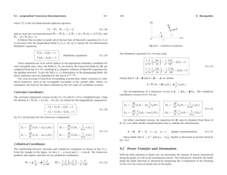
The boundary conditions are that Ey vanish on the right wall, x = a, and that Ex
vanish on the top wall, y = b, that is,
Ey(a, y)= E0y sin kxa cos kyy = 0 , Ex(x, b)= E0x cos kxx sin kyb = 0
The conditions require that kxa and kyb be integral multiples of π:
kxa = nπ , kyb = mπ ⇒ kx =
nπ
a
, ky =
mπ
b
(9.5.6)
These correspond to the TEnm modes. Thus, the cutoff wavenumbers of these modes
kc =

k2
x + k2
y take on the quantized values:
kc =

nπ
a
2
+

mπ
b
2
(TEnm modes) (9.5.7)
The cutoff frequencies fnm = ωc/2π = ckc/2π and wavelengths λnm = c/fnm are:
fnm = c

n
2a
2
+

m
2b
2
, λnm =
1

n
2a
2
+

m
2b
2
(9.5.8)
The TE0m modes are similar to the TEn0 modes, but with x and a replaced by y and
b. The family of TM modes can also be constructed in a similar fashion from Eq. (9.3.10).
Assuming Ez(x, y)= F(x)G(y), we obtain the same equations (9.5.2). Because Ez
is parallel to all walls, we must now choose the solutions sin kx and sin kyy. Thus, the
longitudinal electric fields is:
Ez(x, y)= E0 sin kxx sin kyy (TMnm modes) (9.5.9)
The rest of the field components can be worked out from Eq. (9.3.10) and one finds
that they are given by the same expressions as (9.5.5), except now the constants are
determined in terms of E0:
E1 = −
jβkx
k2
c
E0 , E2 = −
jβky
k2
c
E0
H1 = −
1
ηTM
E2 =
jωky
ωckc
1
η
E0 , H2 =
1
ηTM
E1 = −
jωkx
ωckc
1
η
H0
where we used ηTM = ηβc/ω. The boundary conditions on Ex, Ey are the same as
before, and in addition, we must require that Ez vanish on all walls.
These conditions imply that kx, ky will be given by Eq. (9.5.6), except both n and m
must be non-zero (otherwise Ez would vanish identically.) Thus, the cutoff frequencies
and wavelengths are the same as in Eq. (9.5.8).
Waveguide modes can be excited by inserting small probes at the beginning of the
waveguide. The probes are chosen to generate an electric field that resembles the field
of the desired mode.
378 9. Waveguides
9.6 Operating Bandwidth
All waveguiding systems are operated in a frequency range that ensures that only the
lowest mode can propagate. If several modes can propagate simultaneously,†
one has
no control over which modes will actually be carrying the transmitted signal. This may
cause undue amounts of dispersion, distortion, and erratic operation.
A mode with cutoff frequency ωc will propagate only if its frequency is ω ≥ ωc,
or λ λc. If ω ωc, the wave will attenuate exponentially along the guide direction.
This follows from the ω, β relationship (9.1.10):
ω2
= ω2
c + β2
c2
⇒ β2
=
ω2
− ω2
c
c2
If ω ≥ ωc, the wavenumber β is real-valued and the wave will propagate. But if
ω ωc, β becomes imaginary, say, β = −jα, and the wave will attenuate in the z-
direction, with a penetration depth δ = 1/α:
e−jβz
= e−αz
If the frequency ω is greater than the cutoff frequencies of several modes, then all
of these modes can propagate. Conversely, if ω is less than all cutoff frequencies, then
none of the modes can propagate.
If we arrange the cutoff frequencies in increasing order, ωc1 ωc2 ωc3 · · · ,
then, to ensure single-mode operation, the frequency must be restricted to the interval
ωc1 ω ωc2, so that only the lowest mode will propagate. This interval defines the
operating bandwidth of the guide.
These remarks apply to all waveguiding systems, not just hollow conducting wave-
guides. For example, in coaxial cables the lowest mode is the TEM mode having no cutoff
frequency, ωc1 = 0. However, TE and TM modes with non-zero cutoff frequencies do
exist and place an upper limit on the usable bandwidth of the TEM mode. Similarly, in
optical fibers, the lowest mode has no cutoff, and the single-mode bandwidth is deter-
mined by the next cutoff frequency.
In rectangular waveguides, the smallest cutoff frequencies are f10 = c/2a, f20 =
c/a = 2f10, and f01 = c/2b. Because we assumed that b ≤ a, it follows that always
f10 ≤ f01. If b ≤ a/2, then 1/a ≤ 1/2b and therefore, f20 ≤ f01, so that the two lowest
cutoff frequencies are f10 and f20.
On the other hand, if a/2 ≤ b ≤ a, then f01 ≤ f20 and the two smallest frequencies
are f10 and f01 (except when b = a, in which case f01 = f10 and the smallest frequencies
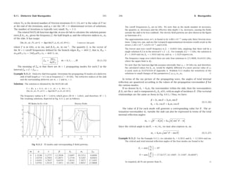
are f10 and f20.) The two cases b ≤ a/2 and b ≥ a/2 are depicted in Fig. 9.6.1.
It is evident from this figure that in order to achieve the widest possible usable
bandwidth for the TE10 mode, the guide dimensions must satisfy b ≤ a/2 so that the
bandwidth is the interval [fc, 2fc], where fc = f10 = c/2a. In terms of the wavelength
λ = c/f, the operating bandwidth becomes: 0.5 ≤ a/λ ≤ 1, or, a ≤ λ ≤ 2a.
We will see later that the total amount of transmitted power in this mode is propor-
tional to the cross-sectional area of the guide, ab. Thus, if in addition to having the
†Murphy’s law for waveguides states that “if a mode can propagate, it will.”

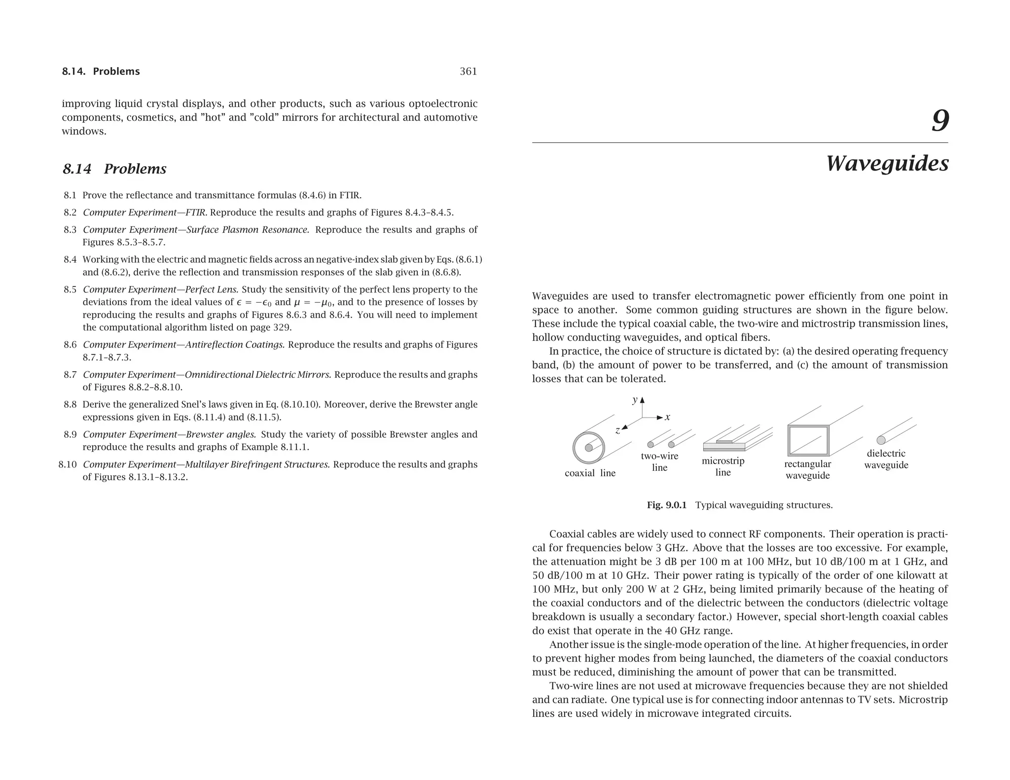
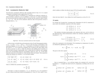
9.7. Power Transfer, Energy Density, and Group Velocity 379
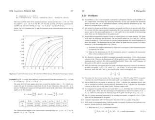
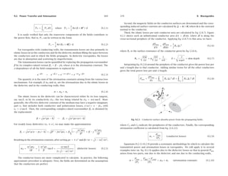
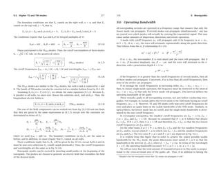
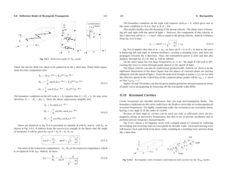
Fig. 9.6.1 Operating bandwidth in rectangular waveguides.
widest bandwidth, we also require to have the maximum power transmitted, the dimen-
sion b must be chosen to be as large as possible, that is, b = a/2. Most practical guides
follow these side proportions.
If there is a “canonical” guide, it will have b = a/2 and be operated at a frequency
that lies in the middle of the operating band [fc, 2fc], that is,
f = 1.5fc = 0.75
c
a
(9.6.1)
Table 9.6.1 lists some standard air-filled rectangular waveguides with their naming
designations, inner side dimensions a, b in inches, cutoff frequencies in GHz, minimum
and maximum recommended operating frequencies in GHz, power ratings, and attenua-
tions in dB/m (the power ratings and attenuations are representative over each operating
band.) We have chosen one example from each microwave band.
name a b fc fmin fmax band P α
WR-510 5.10 2.55 1.16 1.45 2.20 L 9 MW 0.007
WR-284 2.84 1.34 2.08 2.60 3.95 S 2.7 MW 0.019
WR-159 1.59 0.795 3.71 4.64 7.05 C 0.9 MW 0.043
WR-90 0.90 0.40 6.56 8.20 12.50 X 250 kW 0.110
WR-62 0.622 0.311 9.49 11.90 18.00 Ku 140 kW 0.176
WR-42 0.42 0.17 14.05 17.60 26.70 K 50 kW 0.370
WR-28 0.28 0.14 21.08 26.40 40.00 Ka 27 kW 0.583
WR-15 0.148 0.074 39.87 49.80 75.80 V 7.5 kW 1.52
WR-10 0.10 0.05 59.01 73.80 112.00 W 3.5 kW 2.74
Table 9.6.1 Characteristics of some standard air-filled rectangular waveguides.
9.7 Power Transfer, Energy Density, and Group Velocity
Next, we calculate the time-averaged power transmitted in the TE10 mode. We also calcu-
late the energy density of the fields and determine the velocity by which electromagnetic
energy flows down the guide and show that it is equal to the group velocity. We recall
that the non-zero field components are:
Hz(x)= H0 cos kcx , Hx(x)= H1 sin kcx , Ey(x)= E0 sin kcx (9.7.1)
380 9. Waveguides
where
H1 =
jβ
kc
H0 , E0 = −ηTE H1 = −jη
ω
ωc
H0 (9.7.2)
The Poynting vector is obtained from the general result of Eq. (9.3.7):
Pz =
1
2ηTE
|ET|2
=
1
2ηTE
|Ey(x)|2
=
1
2ηTE
|E0|2
sin2
kcx
The transmitted power is obtained by integrating Pz over the cross-sectional area
of the guide:
PT =

a
0

b
0
1
2ηTE
|E0|2
sin2
kcx dxdy
Noting the definite integral,

a
0
sin2
kcx dx =

a
0
sin2
πx
a

dx =
a
2
(9.7.3)
and using ηTE = ηω/βc = η/

1 − ω2
c/ω2, we obtain:
PT =
1
4ηTE
|E0|2
ab =
1
4η
|E0|2
ab

1 −
ω2
c
ω2
(transmitted power) (9.7.4)
We may also calculate the distribution of electromagnetic energy along the guide, as
measured by the time-averaged energy density. The energy densities of the electric and
magnetic fields are:
we =
1
2
Re
1
2
E · E∗

=
1
4
|Ey|2
wm =
1
2
Re
1
2
μH · H∗

=
1
4
μ

|Hx|2
+ |Hz|2

Inserting the expressions for the fields, we find:
we =
1
4
|E0|2
sin2
kcx , wm =
1
4
μ

|H1|2
sin2
kcx + |H0|2
cos2
kcx

Because these quantities represent the energy per unit volume, if we integrate them
over the cross-sectional area of the guide, we will obtain the energy distributions per
unit z-length. Using the integral (9.7.3) and an identical one for the cosine case, we find:
W
e =

a
0

b
0
we(x, y) dxdy =

a
0

b
0
1
4
|E0|2
sin2
kcx dxdy =
1
8
|E0|2
ab
W
m =

a
0

b
0
1
4
μ

|H1|2
sin2
kcx + |H0|2
cos2
kcx

dxdy =
1
8
μ

|H1|2
+ |H0|2

ab

9.8. Power Attenuation 381
Although these expressions look different, they are actually equal, W
e = W
m. In-
deed, using the property β2
/k2
c + 1 = (β2
+ k2
c)/k2
c = k2
/k2
c = ω2
/ω2
c and the relation-
ships between the constants in (9.7.1), we find:
μ

|H1|2
+ |H0|2

= μ

|H0|2 β2
k2
c
+ |H0|2

= μ|H0|2 ω2
ω2
c
=
μ
η2
|E0|2
= |E0|2
The equality of the electric and magnetic energies is a general property of wavegui-
ding systems. We also encountered it in Sec. 2.3 for uniform plane waves. The total
energy density per unit length will be:
W
= W
e + W
m = 2W
e =
1
4
|E0|2
ab (9.7.5)
According to the general relationship between flux, density, and transport velocity
given in Eq. (1.6.2), the energy transport velocity will be the ratio ven = PT/W
. Using
Eqs. (9.7.4) and (9.7.5) and noting that 1/η = 1/
√
μ = c, we find:
ven =
PT
W
= c

1 −
ω2
c
ω2
(energy transport velocity) (9.7.6)
This is equal to the group velocity of the propagating mode. For any dispersion
relationship between ω and β, the group and phase velocities are defined by
vgr =
dω
dβ
, vph =
ω
β
(group and phase velocities) (9.7.7)
For uniform plane waves and TEM transmission lines, we have ω = βc, so that vgr =
vph = c. For a rectangular waveguide, we have ω2
= ω2
c + β2
c2
. Taking differentials of
both sides, we find 2ωdω = 2c2
βdβ, which gives:
vgr =
dω
dβ
=
βc2
ω
= c

1 −
ω2
c
ω2
(9.7.8)
where we used Eq. (9.1.10). Thus, the energy transport velocity is equal to the group
velocity, ven = vgr. We note that vgr = βc2
/ω = c2
/vph, or
vgrvph = c2
(9.7.9)
The energy or group velocity satisfies vgr ≤ c, whereas vph ≥ c. Information trans-
mission down the guide is by the group velocity and, consistent with the theory of
relativity, it is less than c.
9.8 Power Attenuation
In this section, we calculate the attenuation coefficient due to the ohmic losses of the
conducting walls following the procedure outlined in Sec. 9.2. The losses due to the
filling dielectric can be determined from Eq. (9.2.5).
382 9. Waveguides
The field expressions (9.4.3) were derived assuming the boundary conditions for
perfectly conducting wall surfaces. The induced surface currents on the inner walls of
the waveguide are given by Js = n̂ × H, where the unit vector n̂ is ±x̂ and ±ŷ on the
left/right and bottom/top walls, respectively.
The surface currents and tangential magnetic fields are shown in Fig. 9.8.1. In par-
ticular, on the bottom and top walls, we have:
Fig. 9.8.1 Currents on waveguide walls.
Js = ±ŷ×H = ±ŷ×(x̂ Hx +ẑHz)= ±(−ẑ Hx +x̂ Hz)= ±(−ẑ H1 sin kcx+x̂ H0 cos kcx)
Similarly, on the left and right walls:
Js = ±x̂ × H = ±x̂ × (x̂ Hx + ẑHz)= ∓ŷ Hz = ∓ŷ H0 cos kcx
At x = 0 and x = a, this gives Js = ∓ŷ(±H0)= ŷ H0. Thus, the magnitudes of the
surface currents are on the four walls:
|Js|2
=

|H0|2
, (left and right walls)
|H0|2
cos2
kcx + |H1|2
sin2
kcx , (top and bottom walls)
The power loss per unit z-length is obtained from Eq. (9.2.8) by integrating |Js|2
around the four walls, that is,
P
loss = 2
1
2
Rs

a
0
|Js|2
dx + 2
1
2
Rs

b
0
|Js|2
dy
= Rs

a
0

|H0|2
cos2
kcx + |H1|2
sin2
kcx

dx + Rs

b
0
|H0|2
dy
= Rs
a
2

|H0|2
+ |H1|2

+ Rsb|H0|2
=
Rsa
2

|H0|2
+ |H1|2
+
2b
a
|H0|2

Using |H0|2
+|H1|2
= |E0|2
/η2
from Sec. 9.7, and |H0|2
= (|E0|2
/η2
)ω2
c/ω2
, which
follows from Eq. (9.4.2), we obtain:
P
loss =
Rsa|E0|2
2η2

1 +
2b
a
ω2
c
ω2

The attenuation constant is computed from Eqs. (9.2.9) and (9.7.4):

9.8. Power Attenuation 383
αc =
P
loss
2PT
=
Rsa|E0|2
2η2

1 +
2b
a
ω2
c
ω2

2
1
4η
|E0|2
ab

1 −
ω2
c
ω2
which gives:
αc =
Rs
ηb

1 +
2b
a
ω2
c
ω2

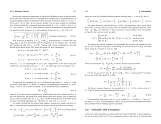
1 −
ω2
c
ω2
(attenuation of TE10 mode) (9.8.1)
This is in units of nepers/m. Its value in dB/m is obtained by αdB = 8.686αc. For a
given ratio a/b, αc increases with decreasing b, thus the smaller the guide dimensions,
the larger the attenuation. This trend is noted in Table 9.6.1.
The main tradeoffs in a waveguiding system are that as the operating frequency f
increases, the dimensions of the guide must decrease in order to maintain the operat-
ing band fc ≤ f ≤ 2fc, but then the attenuation increases and the transmitted power
decreases as it is proportional to the guide’s area.
Example 9.8.1: Design a rectangular air-filled waveguide to be operated at 5 GHz, then, re-
design it to be operated at 10 GHz. The operating frequency must lie in the middle of the
operating band. Calculate the guide dimensions, the attenuation constant in dB/m, and
the maximum transmitted power assuming the maximum electric field is one-half of the
dielectric strength of air. Assume copper walls with conductivity σ = 5.8×107
S/m.
Solution: If f is in the middle of the operating band, fc ≤ f ≤ 2fc, where fc = c/2a, then
f = 1.5fc = 0.75c/a. Solving for a, we find
a =
0.75c
f
=
0.75×30 GHz cm
5
= 4.5 cm
For maximum power transfer, we require b = a/2 = 2.25 cm. Because ω = 1.5ωc, we
have ωc/ω = 2/3. Then, Eq. (9.8.1) gives αc = 0.037 dB/m. The dielectric strength of air
is 3 MV/m. Thus, the maximum allowed electric field in the guide is E0 = 1.5 MV/m. Then,
Eq. (9.7.4) gives PT = 1.12 MW.
At 10 GHz, because f is doubled, the guide dimensions are halved, a = 2.25 and b = 1.125
cm. Because Rs depends on f like f1/2
, it will increase by a factor of
√
2. Then, the factor
Rs/b will increase by a factor of 2
√
2. Thus, the attenuation will increase to the value
αc = 0.037 · 2
√
2 = 0.104 dB/m. Because the area ab is reduced by a factor of four, so
will the power, PT = 1.12/4 = 0.28 MW = 280 kW.
The results of these two cases are consistent with the values quoted in Table 9.6.1 for the
C-band and X-band waveguides, WR-159 and WR-90.

Example 9.8.2: WR-159 Waveguide. Consider the C-band WR-159 air-filled waveguide whose
characteristics were listed in Table 9.6.1. Its inner dimensions are a = 1.59 and b = a/2 =
0.795 inches, or, equivalently, a = 4.0386 and b = 2.0193 cm.
384 9. Waveguides
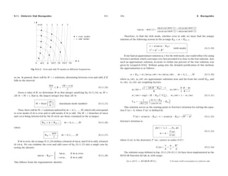
The cutoff frequency of the TE10 mode is fc = c/2a = 3.71 GHz. The maximum operating
bandwidth is the interval [fc, 2fc]= [3.71, 7.42] GHz, and the recommended interval is
[4.64, 7.05] GHz.
Assuming copper walls with conductivity σ = 5.8×107
S/m, the calculated attenuation
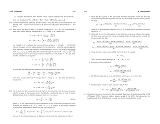
constant αc from Eq. (9.8.1) is plotted in dB/m versus frequency in Fig. 9.8.2.
0 1 2 3 4 5 6 7 8 9 10 11 12
0
0.02
0.04
0.06
0.08
0.1
bandwidth
f (GHz)
α
(dB/m)
Attenuation Coefficient
0 1 2 3 4 5 6 7 8 9 10 11 12
0
0.5
1
1.5
bandwidth
f (GHz)
P
T
(MW)
Power Transmitted
Fig. 9.8.2 Attenuation constant and transmitted power in a WR-159 waveguide.
The power transmitted PT is calculated from Eq. (9.7.4) assuming a maximum breakdown
voltage of E0 = 1.5 MV/m, which gives a safety factor of two over the dielectric breakdown
of air of 3 MV/m. The power in megawatt scales is plotted in Fig. 9.8.2.
Because of the factor

1 − ω2
c/ω2 in the denominator of αc and the numerator of PT,
the attenuation constant becomes very large near the cutoff frequency, while the power is
almost zero. A physical explanation of this behavior is given in the next section.

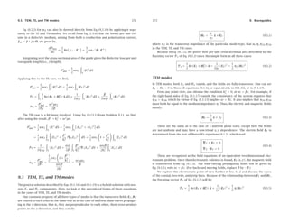
9.9 Reflection Model of Waveguide Propagation
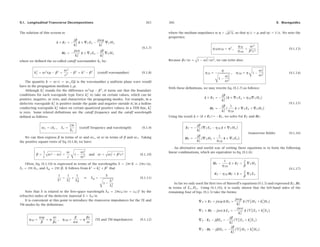
An intuitive model for the TE10 mode can be derived by considering a TE-polarized
uniform plane wave propagating in the z-direction by obliquely bouncing back and forth
between the left and right walls of the waveguide, as shown in Fig. 9.9.1.
If θ is the angle of incidence, then the incident and reflected (from the right wall)
wavevectors will be:
k = x̂ kx + ẑ kz = x̂ k cos θ + ẑ k sin θ
k
= −x̂ kx + ẑ kz = −x̂ k cos θ + ẑ k sin θ
The electric and magnetic fields will be the sum of an incident and a reflected com-
ponent of the form:
E = ŷ E1e−jk·r
+ ŷ E
1e−jk
·r
= ŷ E1e−jkxx
e−jkzz
+ ŷ E
1ejkxx
e−jkzz
= E1 + E
1
H =
1
η
k̂ × E1 +
1
η
k̂

× E
1

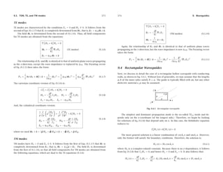
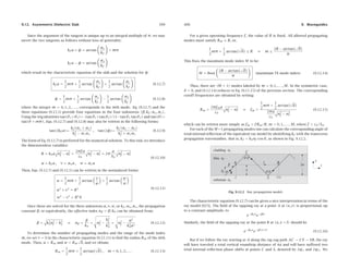
9.9. Reflection Model of Waveguide Propagation 385
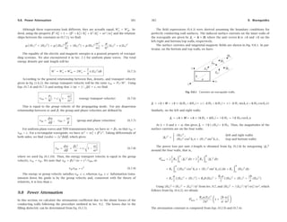
Fig. 9.9.1 Reflection model of TE10 mode.
where the electric field was taken to be polarized in the y direction. These field expres-
sions become component-wise:
Ey =

E1e−jkxx
+ E
1ejkxx

e−jkzz
Hx = −
1
η
sin θ

E1e−jkxx
+ E
1ejkxx

e−jkzz
Hz =
1
η
cos θ

E1e−jkxx
− E
1ejkxx

e−jkzz
(9.9.1)
The boundary condition on the left wall, x = 0, requires that E1 + E
1 = 0. We may write
therefore, E1 = −E
1 = jE0/2. Then, the above expressions simplify into:
Ey = E0 sin kxx e−jkzz
Hx = −
1
η
sin θE0 sin kxx e−jkzz
Hz =
j
η
cos θE0 cos kxx e−jkzz
(9.9.2)
These are identical to Eq. (9.4.3) provided we identify β with kz and kc with kx, as
shown in Fig. 9.9.1. It follows from the wavevector triangle in the figure that the angle
of incidence θ will be given by cos θ = kx/k = kc/k, or,
cos θ =
ωc
ω
, sin θ =

1 −
ω2
c
ω2
(9.9.3)
The ratio of the transverse components, −Ey/Hx, is the transverse impedance, which
is recognized to be ηTE. Indeed, we have:
ηTE = −
Ey
Hx
=
η
sin θ
=
η

1 −
ω2
c
ω2
(9.9.4)
386 9. Waveguides
The boundary condition on the right wall requires sin kxa = 0, which gives rise to
the same condition as (9.4.4), that is, kca = nπ.
This model clarifies also the meaning of the group velocity. The plane wave is bounc-
ing left and right with the speed of light c. However, the component of this velocity in
the z-direction will be vz = c sin θ. This is equal to the group velocity. Indeed, it follows
from Eq. (9.9.3) that:
vz = c sin θ = c

1 −
ω2
c
ω2
= vgr (9.9.5)
Eq. (9.9.3) implies also that at ω = ωc, we have sin θ = 0, or θ = 0, that is, the wave
is bouncing left and right at normal incidence, creating a standing wave, and does not
propagate towards the z-direction. Thus, the transmitted power is zero and this also
implies, through Eq. (9.2.9), that αc will be infinite.
On the other hand, for very large frequencies, ω ωc, the angle θ will tend to 90o
,
causing the wave to zoom through guide almost at the speed of light.
The phase velocity can also be understood geometrically. Indeed, we observe in the
rightmost illustration of the above figure that the planes of constant phase are moving
obliquely with the speed of light c. From the indicated triangle at points 1,2,3, we see that
the effective speed in the z-direction of the common-phase points will be vph = c/ sin θ
so that vphvgr = c2
.
Higher TE and TM modes can also be given similar geometric interpretations in terms
of plane waves propagating by bouncing off the waveguide walls [890].
9.10 Resonant Cavities
Cavity resonators are metallic enclosures that can trap electromagnetic fields. The
boundary conditions on the cavity walls force the fields to exist only at certain quantized
resonant frequencies. For highly conducting walls, the resonances are extremely sharp,
having a very high Q of the order of 10,000.
Because of their high Q, cavities can be used not only to efficiently store electro-
magnetic energy at microwave frequencies, but also to act as precise oscillators and to
perform precise frequency measurements.
Fig. 9.10.1 shows a rectangular cavity with z-length equal to l formed by replacing
the sending and receiving ends of a waveguide by metallic walls. A forward-moving wave
will bounce back and forth from these walls, resulting in a standing-wave pattern along
the z-direction.
Fig. 9.10.1 Rectangular cavity resonator (and induced wall currents for the TEn0p mode.)

9.10. Resonant Cavities 387
Because the tangential components of the electric field must vanish at the end-walls,
these walls must coincide with zero crossings of the standing wave, or put differently, an
integral multiple of half-wavelengths must fit along the z-direction, that is, l = pλg/2 =
pπ/β, or β = pπ/l, where p is a non-zero integer. For the same reason, the standing-
wave patterns along the transverse directions require a = nλx/2 and b = mλy/2, or
kx = nπ/a and ky = mπ/b. Thus, all three cartesian components of the wave vector
are quantized, and therefore, so is the frequency of the wave ω = c

k2
x + k2
y + β2 :
ωnmp = c

nπ
a
2
+

mπ
b
2
+

pπ
l
2
(resonant frequencies) (9.10.1)
Such modes are designated as TEnmp or TMnmp. For simplicity, we consider the case
TEn0p. Eqs. (9.3.6) also describe backward-moving waves if one replaces β by −β, which
also changes the sign of ηTE = ηω/βc. Starting with a linear combination of forward
and backward waves in the TEn0 mode, we obtain the field components:
Hz(x, z) = H0 cos kcx

Ae−jβz
+ Bejβz

,
Hx(x, z) = jH1 sin kcx

Ae−jβz
− Bejβz

, H1 =
β
kc
H0
Ey(x, z) = −jE0 sin kcx

Ae−jβz
+ Bejβz

, E0 =
ω
ωc
ηH0
(9.10.2)
where ωc = ckc. By requiring that Ey(x, z) have z-dependence of the form sin βz, the
coefficients A, B must be chosen as A = −B = j/2. Then, Eq. (9.10.2) specializes into:
Hz(x, z) = H0 cos kcx sin βz ,
Hx(x, z) = −H1 sin kcx cos βz , H1 =
β
kc
H0
Ey(x, z) = −jE0 sin kcx sin βz , E0 =
ω
ωc
ηH0
(9.10.3)
As expected, the vanishing of Ey(x, z) on the front/back walls, z = 0 and z = l, and
on the left/right walls, x = 0 and x = a, requires the quantization conditions: β = pπ/l
and kc = nπ/a. The Q of the resonator can be calculated from its definition:
Q = ω
W
Ploss
(9.10.4)
where W is the total time-averaged energy stored within the cavity volume and Ploss is
the total power loss due to the wall ohmic losses (plus other losses, such as dielectric
losses, if present.) The ratio Δω = Ploss/W is usually identified as the 3-dB width of the
resonance centered at frequency ω. Therefore, we may write Q = ω/Δω.
It is easily verified that the electric and magnetic energies are equal, therefore, W
may be calculated by integrating the electric energy density over the cavity volume:
W = 2We = 2
1
4

vol
|Ey(x, z)|2
dx dy dz =
1
2
|E0|2

a
0

b
0

l
0
sin2
kcx cos2
βz dx dy dz
=
1
8
|E0|2
(abl)=
1
8
μ|H0|2 ω2
ω2
c
(abl)=
1
8
μ |H0|2

k2
c + β2
k2
c

(abl)
388 9. Waveguides
where we used the following definite integrals (valid because kc = nπ/a, β = pπ/l) :

a
0
sin2
kcx dx =

a
0
cos2
kcx dx =
a
2
,

l
0
sin2
βz dz =

l
0
cos2
βz dz =
l
2
(9.10.5)
The ohmic losses are calculated from Eq. (9.2.6), integrated over all six cavity sides.
The surface currents induced on the walls are related to the tangential magnetic fields
by Js = n̂ × Htan. The directions of these currents are shown in Fig. 9.10.1. Specifically,
we find for the currents on the six sides:
|Js|2
=
⎧
⎪
⎪
⎨
⎪
⎪
⎩
H2
0 sin2
βz (left right)
H2
0 cos2
kcx sin2
βz + H2
1 sin2
kcx cos2
βz (top bottom)
H2
1 sin2
kcx (front back)
The power loss can be computed by integrating the loss per unit conductor area,
Eq. (9.2.6), over the six wall sides, or doubling the answer for the left, top, and front
sides. Using the integrals (9.10.5), we find:
Ploss =
1
2
Rs

walls
|Js|2
dA = Rs

H2
0
bl
2
+ (H2
0 + H2
1)
al
4
+ H2
1
ab
2

=
1
4
RsH2
0

l(2b + a)+
β2
k2
c
a(2b + l)
(9.10.6)
where we substituted H2
1 = H2
0β2
/k2
c. It follows that the Q-factor will be:
Q = ω
W
Ploss
=
ωμ
2Rs
(k2
c + β2
)(abl)
k2
cl(2b + a)+β2a(2b + l)
For the TEn0p mode we have β = pπ/l and kc = nπ/a. Using Eq. (9.2.7) to replace
Rs in terms of the skin depth δ, we find:
Q =
1
δ
n2
a2
+
p2
l2
n2
a2

2
a
+
1
b

+
p2
l2

2
l
+
1
b
(9.10.7)
The lowest resonant frequency corresponds to n = p = 1. For a cubic cavity, a =
b = l, the Q and the lowest resonant frequency are:
Q =
a
3δ
, ω101 =
cπ
√
2
a
, f101 =
ω
2π
=
c
a
√
2
(9.10.8)
For an air-filled cubic cavity with a = 3 cm, we find f101 = 7.07 GHz, δ = 7.86×10−5
cm, and Q = 12724. As in waveguides, cavities can be excited by inserting small probes
that generate fields resembling a particular mode.
9.11 Dielectric Slab Waveguides
A dielectric slab waveguide is a planar dielectric sheet or thin film of some thickness,
say 2a, as shown in Fig. 9.11.1. Wave propagation in the z-direction is by total internal

9.11. Dielectric Slab Waveguides 389
Fig. 9.11.1 Dielectric slab waveguide.
reflection from the left and right walls of the slab. Such waveguides provide simple
models for the confining mechanism of waves propagating in optical fibers.
The propagating fields are confined primarily inside the slab, however, they also
exist as evanescent waves outside it, decaying exponentially with distance from the slab.
Fig. 9.11.1 shows a typical electric field pattern as a function of x.
For simplicity, we assume that the media to the left and right of the slab are the
same. To guarantee total internal reflection, the dielectric constants inside and outside
the slab must satisfy 1 2, and similarly for the refractive indices, n1 n2.
We only consider TE modes and look for solutions that depend only on the x co-
ordinate. The cutoff wavenumber kc appearing in the Helmholtz equation for Hz(x)
depends on the dielectric constant of the propagation medium, k2
c = ω2
μ−β2
. There-
fore, k2
c takes different values inside and outside the guide:
k2
c1 = ω2
1μ0 − β2
= ω2
0μ0n2
1 − β2
= k2
0n2
1 − β2
(inside)
k2
c2 = ω2
2μ0 − β2
= ω2
0μ0n2
2 − β2
= k2
0n2
2 − β2
(outside)
(9.11.1)
where k0 = ω/c0 is the free-space wavenumber. We note that ω, β are the same inside
and outside the guide. This follows from matching the tangential fields at all times t
and all points z along the slab walls. The corresponding Helmholtz equations in the
regions inside and outside the guide are:
∂2
xHz(x)+k2
c1Hz(x)= 0 for |x| ≤ a
∂2
xHz(x)+k2
c2Hz(x)= 0 for |x| ≥ a
(9.11.2)
Inside the slab, the solutions are sin kc1x and cos kc1x, and outside, sin kc2x and
cos kc2x, or equivalently, e±jkc2x
. In order for the waves to remain confined in the near
vicinity of the slab, the quantity kc2 must be imaginary, for if it is real, the fields would
propagate at large x distances from the slab (they would correspond to the rays refracted
from the inside into the outside.)
If we set kc2 = −jαc, the solutions outside will be e±αcx
. If αc is positive, then only
the solution e−αcx
is physically acceptable to the right of the slab, x ≥ a, and only eαcx
to the left, x ≤ −a. Thus, the fields attenuate exponentially with the transverse distance
390 9. Waveguides
x, and exist effectively within a skin depth distance 1/αc from the slab. Setting kc1 = kc
and kc2 = −jαc, Eqs. (9.11.1) become in this new notation:
k2
c = k2
0n2
1 − β2
−α2
c = k2
0n2
2 − β2
⇒
k2
c = k2
0n2
1 − β2
α2
c = β2
− k2
0n2
2
(9.11.3)
Similarly, Eqs. (9.11.2) read:
∂2
xHz(x)+k2
cHz(x)= 0 for |x| ≤ a
∂2
xHz(x)−α2
cHz(x)= 0 for |x| ≥ a
(9.11.4)
The two solutions sin kcx and cos kcx inside the guide give rise to the so-called even
and odd TE modes (referring to the evenness or oddness of the resulting electric field.)
For the even modes, the solutions of Eqs. (9.11.4) have the form:
Hz(x)=
⎧
⎪
⎪
⎨
⎪
⎪
⎩
H1 sin kcx , if −a ≤ x ≤ a
H2e−αcx
, if x ≥ a
H3eαcx
, if x ≤ −a
(9.11.5)
The corresponding x-components Hx are obtained by applying Eq. (9.3.8) using the
appropriate value for k2
c, that is, k2
c2 = −α2
c outside and k2
c1 = k2
c inside:
Hx(x)=
⎧
⎪
⎪
⎪
⎪
⎪
⎪
⎪
⎪
⎨
⎪
⎪
⎪
⎪
⎪
⎪
⎪
⎪
⎩
−
jβ
k2
c
∂xHz(x)= −
jβ
kc
H1 cos kcx , if −a ≤ x ≤ a
−
jβ
−α2
c
∂xHz(x)= −
jβ
αc
H2e−αcx
, if x ≥ a
−
jβ
−α2
c
∂xHz(x)=
jβ
αc
H3eαcx
, if x ≤ −a
(9.11.6)
The electric fields are Ey(x)= −ηTEHx(x), where ηTE = ωμ0/β is the same inside
and outside the slab. Thus, the electric field has the form:
Ey(x)=
⎧
⎪
⎪
⎨
⎪
⎪
⎩
E1 cos kcx , if −a ≤ x ≤ a
E2e−αcx
, if x ≥ a
E3eαcx
, if x ≤ −a
(even TE modes) (9.11.7)
E1 =
jβ
kc
ηTE H1 , E2 =
jβ
αc
ηTE H2 , E3 = −
jβ
αc
ηTE H3 (9.11.8)
The boundary conditions state that the tangential components of the magnetic and
electric fields, that is, Hz, Ey, are continuous across the dielectric interfaces at x = −a
and x = a. Similarly, the normal components of the magnetic field Bx = μ0Hx and
therefore also Hx must be continuous. Because Ey = −ηTEHx and ηTE is the same in
both media, the continuity of Ey follows from the continuity of Hx. The continuity of
Hz at x = a and x = −a implies that:

9.11. Dielectric Slab Waveguides 391
H1 sin kca = H2e−αca
and − H1 sin kca = H3e−αca
(9.11.9)
Similarly, the continuity of Hx implies (after canceling a factor of −jβ):
1
kc
H1 cos kca =
1
αc
H2e−αca
and
1
kc
H1 cos kca = −
1
αc
H3e−αca
(9.11.10)
Eqs. (9.11.9) and (9.11.10) imply:
H2 = −H3 = H1eαca
sin kca = H1eαca αc
kc
cos kca (9.11.11)
Similarly, we find for the electric field constants:
E2 = E3 = E1eαca
cos kca = E1eαca kc
αc
sin kca (9.11.12)
The consistency of the last equations in (9.11.11) or (9.11.12) requires that:
cos kca =
kc
αc
sin kca ⇒ αc = kc tan kca (9.11.13)
For the odd TE modes, we have for the solutions of Eq. (9.11.4):
Hz(x)=
⎧
⎪
⎪
⎨
⎪
⎪
⎩
H1 cos kcx , if −a ≤ x ≤ a
H2e−αcx
, if x ≥ a
H3eαcx
, if x ≤ −a
(9.11.14)
The resulting electric field is:
Ey(x)=
⎧
⎪
⎪
⎨
⎪
⎪
⎩
E1 sin kcx , if −a ≤ x ≤ a
E2e−αcx
, if x ≥ a
E3eαcx
, if x ≤ −a
(odd TE modes) (9.11.15)
The boundary conditions imply in this case:
H2 = H3 = H1eαca
cos kca = −H1eαca αc
kc
sin kca (9.11.16)
and, for the electric field constants:
E2 = −E3 = E1eαca
sin kca = −E1eαca kc
αc
cos kca (9.11.17)
The consistency of the last equation requires:
αc = −kc cot kca (9.11.18)
392 9. Waveguides
We note that the electric fields Ey(x) given by Eqs. (9.11.7) and (9.11.15) are even or
odd functions of x for the two families of modes. Expressing E2 and E3 in terms of E1,
we summarize the forms of the electric fields in the two cases:
Ey(x)=
⎧
⎪
⎪
⎨
⎪
⎪
⎩
E1 cos kcx , if −a ≤ x ≤ a
E1 cos kca e−αc(x−a)
, if x ≥ a
E1 cos kca eαc(x+a)
, if x ≤ −a
(even TE modes) (9.11.19)
Ey(x)=
⎧
⎪
⎪
⎨
⎪
⎪
⎩
E1 sin kcx , if −a ≤ x ≤ a
E1 sin kca e−αc(x−a)
, if x ≥ a
−E1 sin kca eαc(x+a)
, if x ≤ −a
(odd TE modes) (9.11.20)
Given the operating frequency ω, Eqs. (9.11.3) and (9.11.13) or (9.11.18) provide three
equations in the three unknowns kc, αc, β. To solve them, we add the two equations
(9.11.3) to eliminate β:
α2
c + k2
c = k2
0(n2
1 − n2
2)=
ω2
c2
0
(n2
1 − n2
2) (9.11.21)
Next, we discuss the numerical solutions of these equations. Defining the dimen-
sionless quantities u = kca and v = αca, we may rewrite Eqs. (9.11.13), (9.11.18), and
(9.11.21) in the equivalent forms:
v = u tan u
v2
+ u2
= R2
(even modes) ,
v = −u cot u
v2
+ u2
= R2
(odd modes) (9.11.22)
where R is the normalized frequency variable:
R = k0aNA =
ωa
c0
NA =
2πfa
c0
NA =
2πa
λ
NA (9.11.23)
where NA =

n2
1 − n2
2 is the numerical aperture of the slab and λ = c0/f, the free-space
wavelength.
Because the functions tan u and cot u have many branches, there may be several
possible solution pairs u, v for each value of R. These solutions are obtained at the
intersections of the curves v = u tan u and v = −u cot u with the circle of radius R,
that is, v2
+ u2
= R2
. Fig. 9.11.2 shows the solutions for various values of the radius R
corresponding to various values of ω.
It is evident from the figure that for small enough R, that is, 0 ≤ R π/2, there is
only one solution and it is even.†
For π/2 ≤ R π, there are two solutions, one even
and one odd. For π ≤ R 3π/2, there are three solutions, two even and one odd, and
†for an optical fiber, the single-mode condition reads 2πaNA/λ 2.405, where a is the core radius.

ch09.pdf

More Related Content

Similar to ch09.pdf

Recently uploaded

ch09.pdf