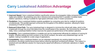
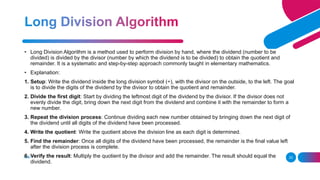
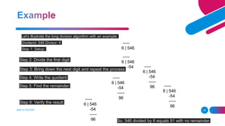
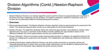
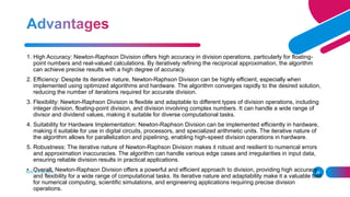
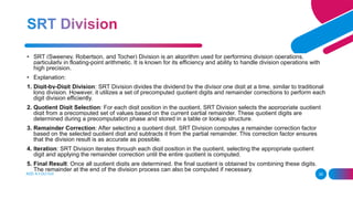
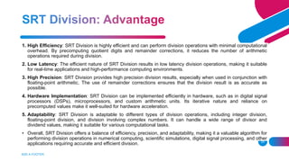
SlideShare a Scribd company logo
Addition, Subtraction,
Multiplication, Division,
Floating Point Operations
Sukesh Kumar Bhagat
DBUU, Dehradun
Computer Arithmetic
2
• Computer arithmetic refers to the set of techniques and methods used by computers to perform arithmetic
operations such as addition, subtraction, multiplication, division, and more complex operations involving real
numbers. It involves the representation of numbers in digital form and the algorithms used to manipulate these
representations to achieve accurate and efficient results.
• In computer arithmetic, numbers are typically represented in binary form, using a finite number of bits to
represent integers, fractions, and real numbers. Various algorithms are employed to perform arithmetic
operations on these representations, taking into account factors such as precision, rounding errors, and
computational efficiency.
• Computer arithmetic is fundamental to all digital computation, playing a crucial role in fields such as computer
science, engineering, physics, finance, and many others. Efficient arithmetic algorithms are essential for
optimizing performance, reducing resource usage, and ensuring the accuracy of computational results in diverse
applications.
Computer Arithmetic
3
1. Performance Optimization: Efficient arithmetic algorithms can significantly enhance the performance of computational tasks by
reducing the time and resources required to perform arithmetic operations. This is particularly important in applications where
large volumes of data need to be processed quickly, such as in scientific simulations, financial modeling, and real-time systems.
2. Resource Utilization: By optimizing arithmetic algorithms, computational resources such as CPU cycles, memory, and energy
can be utilized more effectively. This leads to better utilization of hardware resources, cost savings, and improved scalability of
computational systems.
3. Precision and Accuracy: Efficient arithmetic algorithms ensure that computational results are precise and accurate, minimizing
errors and inaccuracies introduced during calculations. This is especially critical in applications where high levels of accuracy are
required, such as in scientific computing, engineering simulations, and financial calculations.
4. Compatibility and Interoperability: Standardized efficient arithmetic algorithms promote compatibility and interoperability
between different computing systems and platforms. This enables seamless data exchange and communication between diverse
systems, facilitating collaboration and integration of technologies.
5. Scalability: Scalable arithmetic algorithms allow computational systems to handle increasing workloads and larger datasets
without compromising performance or accuracy. This is essential for applications that need to scale up to accommodate growing
demands, such as big data analytics, machine learning, and cloud computing.
6. Real-time Processing: In real-time systems and applications, efficient arithmetic algorithms are essential for meeting strict
timing constraints and deadlines. By minimizing computational overhead and latency, these algorithms enable timely processing
and response to events, ensuring the smooth operation of real-time systems in applications like robotics, automation, and control
systems.
7. Cost-effectiveness: Efficient arithmetic algorithms can lead to cost savings by reducing the hardware requirements and
operational costs associated with computational tasks. This is particularly beneficial in resource-constrained environments and
applications where minimizing costs is a priority.
efficient arithmetic algorithms play a fundamental role in optimizing performance, accuracy, and resource utilization in computational systems,
thereby enabling the development of faster, more reliable, and cost-effective computing solutions across various domains and applications.
•Basic Addition Algorithm
• Step-by-step process
• Examples
•Basic Subtraction Algorithm
• Step-by-step process
• Examples
•Carry Lookahead Addition
• Explanation
• Advantages
•Two's Complement Subtraction
• Explanation
• Advantages
ADD A FOOTER 4
Computer Arithmetic
5
• Step 1: Align the numbers.
• Place the numbers to be added one below the other, aligning them at the rightmost digit (units place). If one
number has more digits than the other, pad the shorter number with zeros to ensure proper alignment.
• Step 2: Start from the rightmost digit (units place).
• Add the digits in the corresponding places (units, tens, hundreds, etc.) together.
• Step 3: Handle carries, if any.
• If the sum of digits in a particular place exceeds 9, carry over the tens place to the left.
• Step 4: Continue adding digits from right to left.
• Repeat steps 2 and 3 for each pair of digits moving from right to left until all digits have been added.
• Step 5: Finalize the sum.
• Once all digits have been added, the final result is obtained.
Computer Arithmetic
6
• Let's add the numbers 235 and 178
• Step 1: Align the numbers.
• Step 2: Start from the rightmost digit (units place).
• Step 3: Handle carries, if any.
• No carry in this step.
• Step 4: Continue adding digits from right to left.
• Step 5: Finalize the sum.
• The sum of 235 and 178 is 413.
• So, 235 + 178 = 413.
235
+ 178
______
235
+ 178
______
235
+ 178
______
3
235
+ 178
______
3 (5+8)
235
+ 178
______
13 (3+7+1)
235
+ 178
______
113 (2+1)
235
+ 178
______
413
Computer Arithmetic
7
• Step 1: Align the numbers.
• Place the numbers to be subtracted one below the other, aligning them at the rightmost digit (units place). If the
second number has fewer digits than the first, pad the shorter number with zeros to ensure proper alignment.
• Step 2: Start from the rightmost digit (units place).
• Subtract the digit in the second number from the corresponding digit in the first number.
• Step 3: Handle borrows, if any.
• If the digit in the first number is smaller than the digit in the second number, borrow from the next higher place
value to the left.
• Step 4: Continue subtracting digits from right to left.
• Repeat steps 2 and 3 for each pair of digits moving from right to left until all digits have been subtracted.
• Step 5: Finalize the difference.
• Once all digits have been subtracted, the final result is obtained.
Computer Arithmetic
8
• Let's subtract 178 from 235.
• Step 1: Align the numbers.
• Step 2: Start from the rightmost digit (units place).
• Step 3: Handle borrows, if any.
No borrow in this step.
• Step 4: Continue subtracting digits from right to left.
• Step 5: Finalize the difference.
• The difference between 235 and 178 is 57.
• So, 235 - 178 = 57.
235
- 178
______
235
- 178
______
235
- 178
______
5
235
- 178
______
57 (3-7)
235
- 178
______
57 (13-8)
235
- 178
______
57 (2-1)
235
- 178
______
57
Computer Arithmetic
9
• Carry Lookahead Addition is a technique used to perform addition in digital circuits, particularly in high-speed
arithmetic units such as ALUs (Arithmetic Logic Units). It's designed to reduce the time required to perform
addition by predicting the carry bits in advance rather than waiting for the carries to propagate through the circuit
sequentially.
• In traditional addition algorithms, carry propagation occurs sequentially from the least significant bit (LSB) to the
most significant bit (MSB). This sequential carry propagation introduces a significant delay, especially in multi-bit
additions, limiting the speed of the addition operation.
• Carry Lookahead Addition, on the other hand, employs a parallel approach to predict carry bits across multiple
stages simultaneously. It divides the addition process into smaller blocks and computes the carry for each block
independently. This allows for predicting whether a carry will be generated or not without waiting for the carry to
propagate through the entire circuit.
• The core concept behind Carry Lookahead Addition lies in generating the carry-out (COUT) for each bit position
based on the input bits and the carry-in (CIN) from the previous bit position. This is achieved using logic gates
such as AND, OR, and XOR gates to compute the carry-out signals for each bit position based on the input
signals.
Computer Arithmetic
10
1. Improved Speed: Carry Lookahead Addition significantly reduces the propagation delay compared to traditional
ripple-carry addition. By predicting carry bits in advance and computing them in parallel, it enables faster
addition operations, making it suitable for high-speed arithmetic units in modern processors.
2. Parallelism: Carry Lookahead Addition exploits parallelism by computing carry bits for multiple bit positions
simultaneously. This parallel approach enhances the throughput of the addition operation, allowing for faster
processing of multi-bit numbers.
3. Reduced Critical Path: The carry lookahead logic is designed to minimize the critical path delay, which is the
longest path through the circuit that determines the overall speed of the operation. By minimizing the critical path
delay, Carry Lookahead Addition further improves the speed and performance of the addition operation.
4. Scalability: Carry Lookahead Addition is scalable and can be implemented efficiently for additions of varying bit
lengths. Whether adding two 8-bit numbers or two 64-bit numbers, the same carry lookahead logic can be
applied, making it suitable for a wide range of applications.
5. Compatibility: Carry Lookahead Addition can be integrated seamlessly into existing digital circuits and
processors, providing a performance boost without requiring significant architectural changes. This makes it a
practical and cost-effective solution for improving the speed and efficiency of arithmetic operations in digital
systems.
Computer Arithmetic
11
• Two's complement subtraction is a method used to subtract one binary number from another using the two's
complement representation. This method is commonly used in digital systems, computers, and processors to
perform subtraction operations efficiently.
1. Representation of Numbers: In two's complement representation, negative numbers are represented by taking
the two's complement of the corresponding positive numbers. To find the two's complement of a binary number,
invert all the bits (change 0s to 1s and 1s to 0s) and add 1 to the result.
2. Subtraction Process:
1. To subtract a binary number B from another binary number A using two's complement subtraction, take the two's
complement of B and add it to A.
2. This can be done by adding A and the two's complement of B using binary addition.
3. Overflow: Overflow can occur in two's complement subtraction when the result exceeds the representable
range of the number of bits used for representation. Overflow occurs if the signs of the two numbers being
subtracted are the same and the sign of the result is different. For example, subtracting a large negative number
from a small positive number can result in overflow.
Computer Arithmetic
12
1. Simplicity: Two's complement subtraction simplifies the subtraction operation by converting it into an addition
operation. This eliminates the need for a separate subtraction algorithm, reducing complexity in digital circuits
and processors.
2. Efficiency: The two's complement subtraction method is computationally efficient and requires minimal
hardware resources. It can be implemented using basic arithmetic and logic units (ALUs) found in digital
systems and processors, making it suitable for high-speed computation.
3. Compatibility: Two's complement subtraction is compatible with the binary representation used in most digital
systems and computers. It seamlessly integrates with existing arithmetic operations, allowing for efficient
implementation without the need for additional encoding or decoding steps.
4. Negative Numbers Handling: Two's complement representation simplifies the handling of negative numbers in
digital systems. By using the same arithmetic operations for both positive and negative numbers, it streamlines
the design of arithmetic units and facilitates arithmetic operations in signed number systems.
5. Overflow Handling: Two's complement subtraction provides a systematic way to detect and handle overflow
conditions. Overflow detection circuits can be integrated into digital systems to identify when the result of a
subtraction operation exceeds the representable range, ensuring accurate computation and error detection.
ADD A FOOTER 13
• Step-by-step process:
1. Align the numbers: Write the two numbers to be multiplied, one below the other, aligning them at the rightmost
digit (units place). If one number has more digits than the other, align the digits accordingly and pad the shorter
number with zeros to ensure proper alignment.
2. Multiply each digit of the multiplier by each digit of the multiplicand: Start from the rightmost digit (units
place) of the multiplier and multiply it by each digit of the multiplicand, one at a time. Write the intermediate
products below each digit of the multiplier, aligning them at the corresponding place values.
3. Add the intermediate products: Sum up all the intermediate products to obtain the final product.
4. Finalize the product: Check for any carry-over and adjust the final product accordingly.
ADD A FOOTER 14
• Multiplicand: 235 Multiplier: 18
• Step 1: Align the numbers:
• Step 2: Multiply each digit of the multiplier by each digit of the multiplicand:
• Step 3: Add the intermediate products
• Step 4: Finalize the product:
• There are no carry-overs, so the final product is:
• So, 235 multiplied by 18 equals 4230.
235
x 18
------
235
x 18
------
000 (Product of 8 and 235)
1880 (Product of 1 and 235, shifted one position to the left)
------
235
x 18
------
000
+ 1880
------
4230
235
x 18
------
4230
ADD A FOOTER 15
• Karatsuba Algorithm is a fast multiplication algorithm that efficiently multiplies two large integers by recursively
breaking down the multiplication into smaller multiplications. It was developed by Anatolii Alexeevitch Karatsuba
in 1960.
• Overview:
1. Divide and Conquer Approach: The Karatsuba Algorithm follows a divide and conquer approach to multiply
two numbers. Instead of directly multiplying the two numbers, it splits them into smaller parts and recursively
computes the product of these smaller parts.
2. Recursive Multiplication: The algorithm splits each number into two halves and recursively computes the
product of these halves. It then combines these partial products to obtain the final result.
3. Combining Partial Products: To combine the partial products efficiently, the algorithm utilizes a clever
technique that reduces the number of multiplications required.
4. Time Complexity: The time complexity of the Karatsuba Algorithm is O(n^log2(3)), which is approximately
O(n^1.585). This makes it more efficient than the traditional grade school method for large numbers.
ADD A FOOTER 16
1. Improved Efficiency: The Karatsuba Algorithm offers improved efficiency for multiplying large numbers
compared to traditional methods like the grade school method. By reducing the number of required
multiplications and employing a divide and conquer strategy, it achieves faster multiplication.
2. Reduced Number of Multiplications: One of the key advantages of the Karatsuba Algorithm is its ability to
reduce the number of required multiplications. This is accomplished by breaking down the multiplication into
smaller multiplications and combining the results using addition and subtraction.
3. Optimized for Large Numbers: The Karatsuba Algorithm is particularly well-suited for multiplying large
integers, where the efficiency gains become more significant compared to traditional methods. It allows for
efficient multiplication of numbers with a large number of digits.
4. Parallelization: The divide and conquer nature of the Karatsuba Algorithm lends itself well to parallelization. The
independent subproblems can be solved in parallel, leading to further improvements in performance on multi-
core or parallel computing architectures.
5. Space Complexity: While the Karatsuba Algorithm offers improved time complexity, it may have slightly higher
space complexity due to the recursive nature of the algorithm. However, the space overhead is generally
manageable and does not outweigh the benefits of faster multiplication.
• Overall, the Karatsuba Algorithm provides a balance between time complexity and space complexity, offering
significant efficiency gains for large integer multiplication tasks. It has become a standard algorithm used in
many applications requiring efficient multiplication of large numbers.
ADD A FOOTER 17
• Booth's Algorithm is a multiplication algorithm used to multiply two signed binary numbers efficiently. It was developed
by Andrew Donald Booth in 1950 and is particularly useful for multiplying large binary numbers in digital circuits and
processors.
1. Binary Multiplication: Booth's Algorithm is designed specifically for binary multiplication. It operates on two signed
binary numbers, the multiplier (M) and the multiplicand (Q), to produce their product.
2. Algorithm Steps:
1. Step 1: Initialize the product (P) to 0.
2. Step 2: Repeat the following steps for each bit position in the multiplier and multiplicand:
1. Check the two rightmost bits of the multiplier and select an operation based on their values (00, 01, 10, or 11).
2. Perform the corresponding operation: no operation, add the multiplicand to the product, subtract the multiplicand from the product, or no operation.
3. Right shift the multiplier and product by one bit position.
3. Handling Signed Numbers: Booth's Algorithm handles signed numbers by using a modified representation of negative
numbers called Booth encoding. This encoding reduces the number of bit transitions and simplifies the multiplication
process.
4. Optimization: Booth's Algorithm optimizes the multiplication process by reducing the number of additions and
subtractions required compared to traditional methods. It achieves this optimization by identifying patterns in the
multiplier and selecting the appropriate operations accordingly.
ADD A FOOTER 18
• :
1. Efficiency: Booth's Algorithm is more efficient than traditional multiplication methods for large binary numbers. By
identifying and exploiting patterns in the multiplier, it reduces the number of additions and subtractions required, leading
to faster multiplication.
2. Simplicity of Hardware Implementation: Booth's Algorithm can be implemented efficiently in digital circuits and
processors using simple hardware components such as adders, shift registers, and control logic. This makes it suitable
for hardware implementations in microprocessors and application-specific integrated circuits (ASICs).
3. Reduced Complexity: Compared to other multiplication algorithms, Booth's Algorithm offers reduced complexity in
terms of both time and space. Its simple and systematic approach simplifies the multiplication process and reduces the
number of required operations.
4. Support for Signed Numbers: Booth's Algorithm inherently supports signed binary numbers through Booth encoding,
allowing for efficient multiplication of both positive and negative numbers without requiring additional sign extension or
conversion steps.
5. Scalability: Booth's Algorithm is scalable and can be applied to multiply binary numbers of varying lengths, from small
numbers to large numbers with hundreds or thousands of bits. It can handle arbitrary precision multiplication efficiently,
making it suitable for a wide range of applications.
• Overall, Booth's Algorithm provides an efficient and scalable solution for binary multiplication, making it a widely used
algorithm in digital systems, processors, and hardware accelerators where efficient multiplication is essential.
ADD A FOOTER 19
• Array Multiplier is a type of hardware multiplier used to perform multiplication of two numbers in digital circuits
and processors. It utilizes an array of logic gates to efficiently compute the product of two multi-bit numbers.
• Overview:
1. Architecture: The Array Multiplier consists of a grid or array of logic gates organized in rows and columns. Each
cell in the array performs a partial product computation by multiplying corresponding bits of the two input
numbers.
2. Partial Products: The Array Multiplier generates partial products for each pair of bits in the multiplicand and
multiplier. These partial products are then added together to obtain the final product.
3. Multiplication Process: The multiplication process in an Array Multiplier is typically performed in parallel, with
all partial products being computed simultaneously. This parallelism enables faster multiplication compared to
sequential algorithms.
4. Carry Propagation: After generating the partial products, the Array Multiplier performs carry propagation to add
the partial products and obtain the final result. This may involve carry-save addition followed by carry
propagation to handle carries between adjacent bits.
ADD A FOOTER 20
1. Digital Signal Processing (DSP): Array Multipliers are commonly used in DSP applications such as filtering,
convolution, and Fourier transforms, where fast and efficient multiplication of large numbers is essential for processing
digital signals in real-time.
2. Microprocessors and CPUs: Array Multipliers are integrated into microprocessors and CPUs to perform arithmetic
operations, including integer and floating-point multiplication. They are essential components of arithmetic logic units
(ALUs) and floating-point units (FPUs) in modern processors.
3. Digital Communication Systems: Array Multipliers play a crucial role in digital communication systems for tasks such
as error correction coding, modulation, and demodulation, where multiplication operations are performed on large
numbers of data bits.
4. Graphics Processing Units (GPUs): In graphics rendering and processing, Array Multipliers are used to perform
matrix multiplications, transformations, and other computational tasks required for rendering complex 3D graphics and
visual effects in real-time.
5. Cryptographic Systems: Array Multipliers are utilized in cryptographic systems for operations such as modular
exponentiation, elliptic curve cryptography, and cryptographic hashing, where fast and efficient multiplication is essential
for securing data and communications.
6. High-Performance Computing (HPC): In scientific simulations, numerical analysis, and other HPC applications, Array
Multipliers are employed to perform matrix operations, linear algebra computations, and other mathematical operations
required for complex simulations and computations.
• Overall, Array Multipliers are versatile and widely used components in digital systems and processors, providing
efficient and scalable solutions for performing multiplication operations in various applications across diverse domains.
ADD A FOOTER 21
• Step-by-step process:
1. Align the numbers: Write the dividend (number to be divided) and the divisor (number by which the dividend is
to be divided) one below the other, aligning them at the leftmost digit.
2. Divide the dividend by the divisor: Begin with the leftmost digit of the dividend and divide it by the divisor to
obtain the quotient and remainder.
3. Write the quotient and remainder: Write the quotient above the division line and the remainder next to the next
digit of the dividend.
4. Repeat the process: Continue dividing the new number formed by combining the remainder and the next digit
of the dividend until all digits of the dividend have been processed.
5. Finalize the quotient: Once all digits of the dividend have been processed, the quotient is obtained by
combining all the individual quotients obtained in each step.
6. Check for correctness: Verify the correctness of the division by multiplying the quotient by the divisor and
adding the remainder. The result should equal the dividend.
ADD A FOOTER 22
• Let's illustrate the basic division algorithm with an example:
• Dividend: 135
• Divisor: 5
• Step 1: Align the numbers
• Step 2: Divide the first digit of the dividend by the divisor:
• Step 3: Multiply the divisor by the quotient and subtract from the dividend to find the remainder:
• Step 4: Repeat the process with the next digit of the dividend:
• Step 5: Finalize the quotient:
• So, 135 divided by 5 equals 27 with a remainder of 0.
135
-----
5 |
135
-----
5 | 2
135
-----
5 | 27
-25
-----
10
135
-----
5 | 27
-25
-----
105
-100
-----
5
135
-----
5 | 27
-25
-----
105
-100
-----
5
Note: In this example, there is no remainder. If there is a
remainder, it should be written as part of the final quotient.
ADD A FOOTER 23
• Long Division Algorithm is a method used to perform division by hand, where the dividend (number to be
divided) is divided by the divisor (number by which the dividend is to be divided) to obtain the quotient and
remainder. It is a systematic and step-by-step approach commonly taught in elementary mathematics.
• Explanation:
1. Setup: Write the dividend inside the long division symbol (÷), with the divisor on the outside, to the left. The goal
is to divide the digits of the dividend by the divisor to obtain the quotient and remainder.
2. Divide the first digit: Start by dividing the leftmost digit of the dividend by the divisor. If the divisor does not
evenly divide the digit, bring down the next digit from the dividend and combine it with the remainder to form a
new number.
3. Repeat the division process: Continue dividing each new number obtained by bringing down the next digit of
the dividend until all digits of the dividend have been processed.
4. Write the quotient: Write the quotient above the division line as each digit is determined.
5. Find the remainder: Once all digits of the dividend have been processed, the remainder is the final value left
after the division process is complete.
6. Verify the result: Multiply the quotient by the divisor and add the remainder. The result should equal the
dividend.
ADD A FOOTER 24
• Let's illustrate the long division algorithm with an example:
• Dividend: 546 Divisor: 6
• Step 1: Setup:
-----
6 | 546
Step 2: Divide the first digit:
-----
6 | 546
-54
Step 3: Bring down the next digit and repeat the process:
-----
6 | 546
-54
-----
96
Step 4: Write the quotient:
-----
6 | 546
-54
-----
96
Step 5: Find the remainder:
-----
6 | 546
-54
-----
96
Step 6: Verify the result:
-----
6 | 546
-54
-----
96 So, 546 divided by 6 equals 91 with no remainder.
ADD A FOOTER 25
• Newton-Raphson Division is an iterative algorithm used to perform division by approximating the reciprocal of
the divisor and then multiplying it by the dividend. It is based on Newton's method for finding the roots of a
function and is particularly useful for dividing floating-point numbers.
• Overview:
1. Reciprocal Approximation: The Newton-Raphson Division algorithm starts by approximating the reciprocal of the
divisor. This reciprocal approximation serves as an initial guess for the division operation.
2. Iteration Process: The algorithm iteratively refines the reciprocal approximation using Newton's method until a
desired level of accuracy is achieved. Each iteration involves updating the approximation based on the
difference between the current approximation and the true reciprocal value.
3. Division Operation: Once an accurate enough reciprocal approximation is obtained, the algorithm performs the
division by multiplying the reciprocal by the dividend. This multiplication step effectively divides the dividend by
the divisor.
4. Handling Remainders: Newton-Raphson Division may also handle remainders by iteratively refining the
reciprocal approximation to obtain more accurate results. Remainders can be handled by adjusting the final
result based on the remainder value obtained during the division process.
Division Algorithms (Contd.):Newton-Raphson
Division
ADD A FOOTER 26
1. High Accuracy: Newton-Raphson Division offers high accuracy in division operations, particularly for floating-
point numbers and real-valued calculations. By iteratively refining the reciprocal approximation, the algorithm
can achieve precise results with a high degree of accuracy.
2. Efficiency: Despite its iterative nature, Newton-Raphson Division can be highly efficient, especially when
implemented using optimized algorithms and hardware. The algorithm converges rapidly to the desired solution,
reducing the number of iterations required for accurate division.
3. Flexibility: Newton-Raphson Division is flexible and adaptable to different types of division operations, including
integer division, floating-point division, and division involving complex numbers. It can handle a wide range of
divisor and dividend values, making it suitable for diverse computational tasks.
4. Suitability for Hardware Implementation: Newton-Raphson Division can be implemented efficiently in hardware,
making it suitable for use in digital circuits, processors, and specialized arithmetic units. The iterative nature of
the algorithm allows for parallelization and pipelining, enabling high-speed division operations in hardware.
5. Robustness: The iterative nature of Newton-Raphson Division makes it robust and resilient to numerical errors
and approximation inaccuracies. The algorithm can handle various edge cases and irregularities in input data,
ensuring reliable division results in practical applications.
• Overall, Newton-Raphson Division offers a powerful and efficient approach to division, providing high accuracy
and flexibility for a wide range of computational tasks. Its iterative nature and adaptability make it a valuable tool
for numerical computing, scientific simulations, and engineering applications requiring precise division
operations.
ADD A FOOTER 27
ADD A FOOTER 28
• SRT (Sweeney, Robertson, and Tocher) Division is an algorithm used for performing division operations,
particularly in floating-point arithmetic. It is known for its efficiency and ability to handle division operations with
high precision.
• Explanation:
1. Digit-by-Digit Division: SRT Division divides the dividend by the divisor one digit at a time, similar to traditional
long division. However, it utilizes a set of precomputed quotient digits and remainder corrections to perform each
digit division efficiently.
2. Quotient Digit Selection: For each digit position in the quotient, SRT Division selects the appropriate quotient
digit from a precomputed set of values based on the current partial remainder. These quotient digits are
determined during a precomputation phase and stored in a table or lookup structure.
3. Remainder Correction: After selecting a quotient digit, SRT Division computes a remainder correction factor
based on the selected quotient digit and subtracts it from the partial remainder. This correction factor ensures
that the division result is as accurate as possible.
4. Iteration: SRT Division iterates through each digit position in the quotient, selecting the appropriate quotient
digit and applying the remainder correction until the entire quotient is computed.
5. Final Result: Once all quotient digits are determined, the final quotient is obtained by combining these digits.
The remainder at the end of the division process can also be computed if necessary.
ADD A FOOTER
29
1. High Efficiency: SRT Division is highly efficient and can perform division operations with minimal computational
overhead. By precomputing quotient digits and remainder corrections, it reduces the number of arithmetic
operations required during division.
2. Low Latency: The efficient nature of SRT Division results in low latency division operations, making it suitable
for real-time applications and high-performance computing environments.
3. High Precision: SRT Division provides high precision division results, especially when used in conjunction with
floating-point arithmetic. The use of remainder corrections ensures that the division result is as accurate as
possible.
4. Hardware Implementation: SRT Division can be implemented efficiently in hardware, such as in digital signal
processors (DSPs), microprocessors, and custom arithmetic units. Its iterative nature and reliance on
precomputed values make it well-suited for hardware acceleration.
5. Adaptability: SRT Division is adaptable to different types of division operations, including integer division,
floating-point division, and division involving complex numbers. It can handle a wide range of divisor and
dividend values, making it suitable for various computational tasks.
• Overall, SRT Division offers a balance of efficiency, precision, and adaptability, making it a valuable algorithm for
performing division operations in numerical computing, scientific simulations, digital signal processing, and other
applications requiring accurate and efficient division.
ADD A FOOTER 30
ADD A FOOTER 31
Floating point representation is a method used to represent real numbers in computing systems, particularly in
floating-point arithmetic. It consists of three components: sign, exponent, and mantissa.
1. Sign: The sign bit indicates whether the number is positive or negative. It is typically represented using one bit,
where 0 denotes a positive number and 1 denotes a negative number.
2. Exponent: The exponent represents the scale or magnitude of the number. It is typically represented using a
fixed number of bits, allowing the representation of a wide range of magnitudes. The exponent bias is added to
the actual exponent to allow for both positive and negative exponents.
3. Mantissa: The mantissa (also known as significand or fraction) represents the precision or fractional part of the
number. It is typically represented using a fixed number of bits and contains the significant digits of the number.
ADD A FOOTER 32
• The floating point addition algorithm combines two floating point numbers (operands) to produce a single floating
point result. It involves aligning the operands, adjusting the exponents, performing the addition or subtraction of
the mantissas, and normalizing the result.
1. Align the operands: Align the operands by adjusting the exponents so that they have the same exponent value.
This may involve shifting the mantissa and adjusting the exponent accordingly.
2. Perform addition or subtraction: Add or subtract the aligned mantissas based on the sign of the operands. If
the signs are different, perform subtraction; if the signs are the same, perform addition.
3. Normalize the result: Normalize the result by adjusting the mantissa and exponent to ensure that the leading
bit of the mantissa is 1 and the exponent is within the valid range.
4. Check for overflow or underflow: Check if the result exceeds the range of representable numbers. If the result
is too large (overflow) or too small (underflow), adjust the exponent and mantissa accordingly.
5. Round the result: Round the result to the desired precision, if necessary, by considering the bits beyond the
precision of the mantissa.
ADD A FOOTER 33
• Let's illustrate the floating point addition algorithm with an example:
• Operand 1: 0.75×23
• Operand 2: 0.5×22
• Step 1: Align the operands:
• 0.75×23=111.0×20
• 0.5×22=1.00×20
• Step 2: Perform addition:
• 111.0+1.00=1000.0
• Step 3: Normalize the result:
• 1000.0×20
• Step 4: Round the result (if necessary).
• So, the result of 0.75×23+0.5×22 is 1.000×20.
ADD A FOOTER 34
• The floating point subtraction algorithm is similar to the floating point addition algorithm, but it involves
subtracting one floating point number from another. It follows similar steps such as aligning the operands,
adjusting the exponents, performing subtraction, normalizing the result, and rounding if necessary.
• Algorithm:
1. Align the operands: Align the operands by adjusting the exponents so that they have the same exponent value.
This may involve shifting the mantissa and adjusting the exponent accordingly.
2. Perform subtraction: Subtract the aligned mantissas based on the sign of the operands. If the signs are
different, perform addition; if the signs are the same, perform subtraction.
3. Normalize the result: Normalize the result by adjusting the mantissa and exponent to ensure that the leading
bit of the mantissa is 1 and the exponent is within the valid range.
4. Check for overflow or underflow: Check if the result exceeds the range of representable numbers. If the result
is too large (overflow) or too small (underflow), adjust the exponent and mantissa accordingly.
5. Round the result: Round the result to the desired precision, if necessary, by considering the bits beyond the
precision of the mantissa.
ADD A FOOTER 35
• Let's illustrate the floating point subtraction algorithm with an example:
• Operand 1: 1.25×23
• Operand 2: 0.5×22
• Step 1: Align the operands:
• 1.25×23=101.0×20
• 0.5×22=1.00×20
• Step 2: Perform subtraction:
• 101.0−1.00=100.0101.0−1.00=100.0
• Step 3: Normalize the result:
• 100.0×20
• Step 4: Round the result (if necessary).
• So, the result of 1.25×23−0.5×22 is 1.00×20.
ADD A FOOTER 36
• The floating point multiplication algorithm involves multiplying two floating point numbers together to obtain a
single floating point result. It follows a series of steps including aligning the exponents, multiplying the
mantissas, adjusting the exponent and mantissa of the result, and rounding if necessary.
• Algorithm:
1. Align the exponents: Align the exponents of the two operands by adjusting one or both of them. This may
involve shifting the mantissa and adjusting the exponent accordingly.
2. Multiply the mantissas: Multiply the aligned mantissas together to obtain the product.
3. Adjust the exponent: Add the exponents of the operands to obtain the exponent of the result. Adjust the
exponent and mantissa of the result to ensure that the leading bit of the mantissa is 1 and the exponent is within
the valid range.
4. Check for overflow or underflow: Check if the result exceeds the range of representable numbers. If the result
is too large (overflow) or too small (underflow), adjust the exponent and mantissa accordingly.
5. Round the result: Round the result to the desired precision, if necessary, by considering the bits beyond the
precision of the mantissa.
ADD A FOOTER 37
• Let's illustrate the floating point multiplication algorithm with an example:
Operand 1: 0.75×23
Operand 2: 0.5×22
• Step 1: Align the exponents:
• 0.75×23=111.0×20
• 0.5×22=1.00×20
• Step 2: Multiply the mantissas:
• 111.0×1.00=111.0
• Step 3: Adjust the exponent:
• 111.0×20
• Step 4: Round the result (if necessary).
So, the result of 0.75×23×0.5×22 is 1.11×20.
ADD A FOOTER 38
• The floating point division algorithm involves dividing one floating point number (dividend) by another (divisor) to
obtain a single floating point result. It follows a series of steps including aligning the exponents, dividing the
mantissas, adjusting the exponent and mantissa of the result, and rounding if necessary.
1. Align the exponents: Align the exponents of the dividend and divisor by adjusting one or both of them. This
may involve shifting the mantissa and adjusting the exponent accordingly.
2. Divide the mantissas: Divide the aligned mantissa of the dividend by the aligned mantissa of the divisor to
obtain the quotient.
3. Adjust the exponent: Subtract the exponent of the divisor from the exponent of the dividend to obtain the
exponent of the result. Adjust the exponent and mantissa of the result to ensure that the leading bit of the
mantissa is 1 and the exponent is within the valid range.
4. Check for overflow or underflow: Check if the result exceeds the range of representable numbers. If the result
is too large (overflow) or too small (underflow), adjust the exponent and mantissa accordingly.
5. Round the result: Round the result to the desired precision, if necessary, by considering the bits beyond the
precision of the mantissa.
ADD A FOOTER 39
Let's illustrate the floating point division algorithm with an example:
• Dividend: 1.25×23
• Divisor: 0.5×22
• Step 1: Align the exponents:
• 1.25×23=101.0×20
• 0.5×22=1.00×20
• Step 2: Divide the mantissas:
• Step 3: Adjust the exponent:
• 101.0×20
• Step 4: Round the result (if necessary).
• So, the result of 1.25×23÷0.5×22 is 101.0×20
ADD A FOOTER 40
• Round-off errors occur in numerical computations when the precision of the representation of numbers is limited,
leading to inaccuracies in the result due to rounding. These errors can accumulate and affect the accuracy of
computations, especially in iterative algorithms or when dealing with large numbers of computations.
1. Limited Precision: Computers represent real numbers using a finite number of bits, which imposes limits on the
precision of numerical computations. When performing arithmetic operations, the result may contain more digits
than can be represented, leading to rounding errors.
2. Rounding: Rounding occurs when a result with more digits than the representation can handle needs to be
truncated or approximated. Rounding can introduce errors, particularly when the discarded digits contain
significant information.
3. Accumulation of Errors: In iterative algorithms or algorithms involving repeated computations, round-off errors
can accumulate, leading to significant deviations from the true solution over time. These accumulated errors can
affect the accuracy and reliability of the computation.
ADD A FOOTER 41
1. Increased Precision: Using higher precision data types, such as double-precision floating-point numbers, can mitigate
round-off errors by allowing for more significant digits to be represented. However, this approach may come with
increased memory and computational costs.
2. Error Analysis: Conducting error analysis to estimate and analyze the impact of round-off errors on the overall
accuracy of the computation can help identify critical areas where errors are likely to accumulate. This information can
inform the development of mitigation strategies.
3. Numerical Algorithms: Choosing numerical algorithms that are less susceptible to round-off errors can help minimize
their impact. For example, algorithms that avoid subtractive cancellation or use stable numerical techniques can reduce
the propagation of errors.
4. Error Bounds: Establishing error bounds and tolerances for numerical computations can provide guidance on
acceptable levels of error and help identify when results may be unreliable due to round-off errors exceeding specified
thresholds.
5. Algorithmic Modifications: Modifying algorithms to minimize the propagation of round-off errors can improve their
numerical stability. This may involve restructuring computations, using alternative formulations, or incorporating error-
correcting techniques.
6. Precision Scaling: Scaling numerical quantities to appropriate ranges before performing computations can help
distribute the precision more evenly and reduce the likelihood of significant digits being lost due to rounding.
7. Error Compensation: Implementing error compensation techniques, such as compensated summation or pairwise
summation, can help mitigate the effects of round-off errors by reducing the loss of precision during summation
operations.
• By employing these mitigation techniques, developers and researchers can effectively manage round-off errors and
maintain the accuracy and reliability of numerical computations in various applications.
Computer Arithmetic
42
1. Financial Modeling: Efficient arithmetic algorithms are crucial in financial modeling for tasks such as portfolio
optimization, risk assessment, and option pricing. High-performance arithmetic operations are required to handle
large datasets and complex mathematical models accurately.
2. Scientific Simulations: In fields such as physics, chemistry, biology, and engineering, efficient arithmetic
algorithms are used to simulate physical processes, conduct numerical simulations, and solve differential
equations. These algorithms enable researchers to model complex systems accurately and analyze
experimental data.
3. Digital Signal Processing (DSP): DSP applications, including audio and image processing,
telecommunications, radar, and sonar, rely on efficient arithmetic algorithms for tasks such as filtering,
convolution, Fourier transforms, and signal analysis. Real-time processing of signals requires high-performance
arithmetic operations to handle large volumes of data efficiently.
4. Computer Graphics: Arithmetic algorithms play a vital role in computer graphics for rendering 2D and 3D
images, performing geometric transformations, shading, texture mapping, and ray tracing. Efficient arithmetic
operations are essential for rendering realistic graphics in video games, animation, virtual reality, and computer-
aided design (CAD) applications.
5. Machine Learning and Artificial Intelligence: In machine learning and AI applications, efficient arithmetic
algorithms are used for training and inference tasks, including matrix operations, optimization algorithms, neural
network computations, and deep learning models. High-performance arithmetic operations enable the efficient
processing of large-scale datasets and complex neural network architectures.
ADD A FOOTER 43
1. Performance Optimization: Efficient arithmetic algorithms are fundamental to performance optimization in
computer systems and engineering applications. By improving the efficiency of arithmetic operations, developers
can enhance the overall performance of software applications, computational models, and hardware systems.
2. Resource Utilization: Efficient arithmetic algorithms help optimize resource utilization in computing systems,
including CPU, memory, and storage resources. By minimizing the computational overhead and memory
footprint of arithmetic operations, developers can maximize the utilization of available resources.
3. Algorithm Design: Efficient arithmetic algorithms inform the design and implementation of algorithms in
computer science and engineering. By understanding the performance characteristics of arithmetic operations,
developers can design algorithms that are scalable, robust, and optimized for specific computational tasks.
4. Hardware Design: In hardware design, efficient arithmetic algorithms influence the architecture and
implementation of digital circuits, processors, and specialized arithmetic units. By designing hardware
components that efficiently execute arithmetic operations, engineers can improve the performance and energy
efficiency of computing systems.
5. Software Development: Efficient arithmetic algorithms are essential for software development in various
domains, including scientific computing, numerical analysis, embedded systems, and high-performance
computing. By leveraging optimized arithmetic algorithms, developers can create software applications that
deliver fast and accurate results.
ADD A FOOTER 44
1. Quantum Computing: The development of quantum computing technologies is expected to revolutionize
arithmetic algorithms by enabling parallel and probabilistic computation. Quantum arithmetic algorithms promise
exponential speedup for certain computational tasks, including factorization, optimization, and simulation.
2. Approximate Computing: Approximate arithmetic algorithms are gaining popularity as a way to trade off
accuracy for efficiency in computational tasks where precise results are not required. Approximate arithmetic
techniques leverage probabilistic and statistical methods to achieve significant improvements in performance
and energy efficiency.
3. Parallel and Distributed Computing: With the proliferation of multi-core processors, GPUs, and distributed
computing platforms, arithmetic algorithms are being adapted to exploit parallelism and distributed computing
techniques. Parallel arithmetic algorithms enable the efficient execution of arithmetic operations across multiple
processing units, leading to faster computation and scalability.
4. Hardware Acceleration: The use of hardware accelerators, such as field-programmable gate arrays (FPGAs),
graphics processing units (GPUs), and application-specific integrated circuits (ASICs), is driving advancements
in arithmetic algorithm optimization. Hardware-accelerated arithmetic algorithms offer significant performance
gains and energy efficiency improvements for compute-intensive applications.
5. Deep Learning and Neural Arithmetic Logic Units (NALUs): In the field of deep learning, neural arithmetic
logic units (NALUs) are emerging as a new approach to arithmetic operations in neural networks. NALUs enable
neural networks to perform arithmetic operations, such as addition, subtraction, multiplication, and division, in a
differentiable manner, facilitating end-to-end training and improved model performance.
Notes: efficient arithmetic algorithms will continue to play a critical role in advancing computer science and engineering, enabling innovations in
various domains, including computational science, artificial intelligence, and quantum computing. As computing technologies evolve, arithmetic
algorithms will evolve to meet the growing demands for performance, efficiency, and scalability in computational tasks.

More Related Content

Similar to Computer Arithmetic Algorithm Arithmetic.pptx

Hennchthree 160912095304
Hennchthree 160912095304Hennchthree 160912095304
Hennchthree 160912095304
marangburu42
 

Similar to Computer Arithmetic Algorithm Arithmetic.pptx (20)

Computer arithmetics (computer organisation & arithmetics) ppt
Computer arithmetics (computer organisation & arithmetics) pptComputer arithmetics (computer organisation & arithmetics) ppt
Computer arithmetics (computer organisation & arithmetics) ppt
 
Hennchthree 160912095304
Hennchthree 160912095304Hennchthree 160912095304
Hennchthree 160912095304
 
Computer arithmetics coa project pdf version
Computer arithmetics coa project pdf versionComputer arithmetics coa project pdf version
Computer arithmetics coa project pdf version
 
A Fast Floating Point Double Precision Implementation on Fpga
A Fast Floating Point Double Precision Implementation on FpgaA Fast Floating Point Double Precision Implementation on Fpga
A Fast Floating Point Double Precision Implementation on Fpga
 
IRJET - Design of a Low Power Serial- Parallel Multiplier with Low Transition...
IRJET - Design of a Low Power Serial- Parallel Multiplier with Low Transition...IRJET - Design of a Low Power Serial- Parallel Multiplier with Low Transition...
IRJET - Design of a Low Power Serial- Parallel Multiplier with Low Transition...
 
Design, Develop and Implement an Efficient Polynomial Divider
Design, Develop and Implement an Efficient Polynomial DividerDesign, Develop and Implement an Efficient Polynomial Divider
Design, Develop and Implement an Efficient Polynomial Divider
 
Hennchthree
HennchthreeHennchthree
Hennchthree
 
High Speed Unified Field Crypto processor for Security Applications using Ver...
High Speed Unified Field Crypto processor for Security Applications using Ver...High Speed Unified Field Crypto processor for Security Applications using Ver...
High Speed Unified Field Crypto processor for Security Applications using Ver...
 
Review on 32 bit single precision Floating point unit (FPU) Based on IEEE 754...
Review on 32 bit single precision Floating point unit (FPU) Based on IEEE 754...Review on 32 bit single precision Floating point unit (FPU) Based on IEEE 754...
Review on 32 bit single precision Floating point unit (FPU) Based on IEEE 754...
 
Problem-solving and design 1.pptx
Problem-solving and design 1.pptxProblem-solving and design 1.pptx
Problem-solving and design 1.pptx
 
Design of a Novel Multiplier and Accumulator using Modified Booth Algorithm w...
Design of a Novel Multiplier and Accumulator using Modified Booth Algorithm w...Design of a Novel Multiplier and Accumulator using Modified Booth Algorithm w...
Design of a Novel Multiplier and Accumulator using Modified Booth Algorithm w...
 
Computer project
Computer projectComputer project
Computer project
 
International Journal of Engineering Research and Development
International Journal of Engineering Research and DevelopmentInternational Journal of Engineering Research and Development
International Journal of Engineering Research and Development
 
VLSI Design of Fast Addition Using QSD Adder for Better Performance
VLSI Design of Fast Addition Using QSD Adder for Better  PerformanceVLSI Design of Fast Addition Using QSD Adder for Better  Performance
VLSI Design of Fast Addition Using QSD Adder for Better Performance
 
Hardware Implementation of Tactile Data Processing Methods for the Reconstruc...
Hardware Implementation of Tactile Data Processing Methods for the Reconstruc...Hardware Implementation of Tactile Data Processing Methods for the Reconstruc...
Hardware Implementation of Tactile Data Processing Methods for the Reconstruc...
 
An Improved Frequent Itemset Generation Algorithm Based On Correspondence
An Improved Frequent Itemset Generation Algorithm Based On Correspondence An Improved Frequent Itemset Generation Algorithm Based On Correspondence
An Improved Frequent Itemset Generation Algorithm Based On Correspondence
 
High Speed Signed multiplier for Digital Signal Processing Applications
High Speed Signed multiplier for Digital Signal Processing ApplicationsHigh Speed Signed multiplier for Digital Signal Processing Applications
High Speed Signed multiplier for Digital Signal Processing Applications
 
IRJET- Literature Survey on Hardware Addition and Subtraction
IRJET- Literature Survey on Hardware Addition and SubtractionIRJET- Literature Survey on Hardware Addition and Subtraction
IRJET- Literature Survey on Hardware Addition and Subtraction
 
Design of Efficient High Speed Vedic Multiplier
Design of Efficient High Speed Vedic MultiplierDesign of Efficient High Speed Vedic Multiplier
Design of Efficient High Speed Vedic Multiplier
 
Algo and flowchart
Algo and flowchartAlgo and flowchart
Algo and flowchart
 

Recently uploaded

Online blood donation management system project.pdf
Online blood donation management system project.pdfOnline blood donation management system project.pdf
Online blood donation management system project.pdf
Kamal Acharya
 
School management system project report.pdf
School management system project report.pdfSchool management system project report.pdf
School management system project report.pdf
Kamal Acharya
 
ONLINE VEHICLE RENTAL SYSTEM PROJECT REPORT.pdf
ONLINE VEHICLE RENTAL SYSTEM PROJECT REPORT.pdfONLINE VEHICLE RENTAL SYSTEM PROJECT REPORT.pdf
ONLINE VEHICLE RENTAL SYSTEM PROJECT REPORT.pdf
Kamal Acharya
 

Recently uploaded (20)

2024 DevOps Pro Europe - Growing at the edge
2024 DevOps Pro Europe - Growing at the edge2024 DevOps Pro Europe - Growing at the edge
2024 DevOps Pro Europe - Growing at the edge
 
Furniture showroom management system project.pdf
Furniture showroom management system project.pdfFurniture showroom management system project.pdf
Furniture showroom management system project.pdf
 
Quality defects in TMT Bars, Possible causes and Potential Solutions.
Quality defects in TMT Bars, Possible causes and Potential Solutions.Quality defects in TMT Bars, Possible causes and Potential Solutions.
Quality defects in TMT Bars, Possible causes and Potential Solutions.
 
Introduction to Machine Learning Unit-4 Notes for II-II Mechanical Engineering
Introduction to Machine Learning Unit-4 Notes for II-II Mechanical EngineeringIntroduction to Machine Learning Unit-4 Notes for II-II Mechanical Engineering
Introduction to Machine Learning Unit-4 Notes for II-II Mechanical Engineering
 
RM&IPR M4.pdfResearch Methodolgy & Intellectual Property Rights Series 4
RM&IPR M4.pdfResearch Methodolgy & Intellectual Property Rights Series 4RM&IPR M4.pdfResearch Methodolgy & Intellectual Property Rights Series 4
RM&IPR M4.pdfResearch Methodolgy & Intellectual Property Rights Series 4
 
NO1 Pandit Black Magic Removal in Uk kala jadu Specialist kala jadu for Love ...
NO1 Pandit Black Magic Removal in Uk kala jadu Specialist kala jadu for Love ...NO1 Pandit Black Magic Removal in Uk kala jadu Specialist kala jadu for Love ...
NO1 Pandit Black Magic Removal in Uk kala jadu Specialist kala jadu for Love ...
 
internship exam ppt.pptx on embedded system and IOT
internship exam ppt.pptx on embedded system and IOTinternship exam ppt.pptx on embedded system and IOT
internship exam ppt.pptx on embedded system and IOT
 
retail automation billing system ppt.pptx
retail automation billing system ppt.pptxretail automation billing system ppt.pptx
retail automation billing system ppt.pptx
 
Research Methodolgy & Intellectual Property Rights Series 2
Research Methodolgy & Intellectual Property Rights Series 2Research Methodolgy & Intellectual Property Rights Series 2
Research Methodolgy & Intellectual Property Rights Series 2
 
Natalia Rutkowska - BIM School Course in Kraków
Natalia Rutkowska - BIM School Course in KrakówNatalia Rutkowska - BIM School Course in Kraków
Natalia Rutkowska - BIM School Course in Kraków
 
Online blood donation management system project.pdf
Online blood donation management system project.pdfOnline blood donation management system project.pdf
Online blood donation management system project.pdf
 
School management system project report.pdf
School management system project report.pdfSchool management system project report.pdf
School management system project report.pdf
 
Supermarket billing system project report..pdf
Supermarket billing system project report..pdfSupermarket billing system project report..pdf
Supermarket billing system project report..pdf
 
Dairy management system project report..pdf
Dairy management system project report..pdfDairy management system project report..pdf
Dairy management system project report..pdf
 
Lect 2 - Design of slender column-2.pptx
Lect 2 - Design of slender column-2.pptxLect 2 - Design of slender column-2.pptx
Lect 2 - Design of slender column-2.pptx
 
The battle for RAG, explore the pros and cons of using KnowledgeGraphs and Ve...
The battle for RAG, explore the pros and cons of using KnowledgeGraphs and Ve...The battle for RAG, explore the pros and cons of using KnowledgeGraphs and Ve...
The battle for RAG, explore the pros and cons of using KnowledgeGraphs and Ve...
 
ONLINE CAR SERVICING SYSTEM PROJECT REPORT.pdf
ONLINE CAR SERVICING SYSTEM PROJECT REPORT.pdfONLINE CAR SERVICING SYSTEM PROJECT REPORT.pdf
ONLINE CAR SERVICING SYSTEM PROJECT REPORT.pdf
 
ONLINE VEHICLE RENTAL SYSTEM PROJECT REPORT.pdf
ONLINE VEHICLE RENTAL SYSTEM PROJECT REPORT.pdfONLINE VEHICLE RENTAL SYSTEM PROJECT REPORT.pdf
ONLINE VEHICLE RENTAL SYSTEM PROJECT REPORT.pdf
 
BRAKING SYSTEM IN INDIAN RAILWAY AutoCAD DRAWING
BRAKING SYSTEM IN INDIAN RAILWAY AutoCAD DRAWINGBRAKING SYSTEM IN INDIAN RAILWAY AutoCAD DRAWING
BRAKING SYSTEM IN INDIAN RAILWAY AutoCAD DRAWING
 
İTÜ CAD and Reverse Engineering Workshop
İTÜ CAD and Reverse Engineering WorkshopİTÜ CAD and Reverse Engineering Workshop
İTÜ CAD and Reverse Engineering Workshop
 

Computer Arithmetic Algorithm Arithmetic.pptx

  • 1. Addition, Subtraction, Multiplication, Division, Floating Point Operations Sukesh Kumar Bhagat DBUU, Dehradun
  • 2. Computer Arithmetic 2 • Computer arithmetic refers to the set of techniques and methods used by computers to perform arithmetic operations such as addition, subtraction, multiplication, division, and more complex operations involving real numbers. It involves the representation of numbers in digital form and the algorithms used to manipulate these representations to achieve accurate and efficient results. • In computer arithmetic, numbers are typically represented in binary form, using a finite number of bits to represent integers, fractions, and real numbers. Various algorithms are employed to perform arithmetic operations on these representations, taking into account factors such as precision, rounding errors, and computational efficiency. • Computer arithmetic is fundamental to all digital computation, playing a crucial role in fields such as computer science, engineering, physics, finance, and many others. Efficient arithmetic algorithms are essential for optimizing performance, reducing resource usage, and ensuring the accuracy of computational results in diverse applications.
  • 3. Computer Arithmetic 3 1. Performance Optimization: Efficient arithmetic algorithms can significantly enhance the performance of computational tasks by reducing the time and resources required to perform arithmetic operations. This is particularly important in applications where large volumes of data need to be processed quickly, such as in scientific simulations, financial modeling, and real-time systems. 2. Resource Utilization: By optimizing arithmetic algorithms, computational resources such as CPU cycles, memory, and energy can be utilized more effectively. This leads to better utilization of hardware resources, cost savings, and improved scalability of computational systems. 3. Precision and Accuracy: Efficient arithmetic algorithms ensure that computational results are precise and accurate, minimizing errors and inaccuracies introduced during calculations. This is especially critical in applications where high levels of accuracy are required, such as in scientific computing, engineering simulations, and financial calculations. 4. Compatibility and Interoperability: Standardized efficient arithmetic algorithms promote compatibility and interoperability between different computing systems and platforms. This enables seamless data exchange and communication between diverse systems, facilitating collaboration and integration of technologies. 5. Scalability: Scalable arithmetic algorithms allow computational systems to handle increasing workloads and larger datasets without compromising performance or accuracy. This is essential for applications that need to scale up to accommodate growing demands, such as big data analytics, machine learning, and cloud computing. 6. Real-time Processing: In real-time systems and applications, efficient arithmetic algorithms are essential for meeting strict timing constraints and deadlines. By minimizing computational overhead and latency, these algorithms enable timely processing and response to events, ensuring the smooth operation of real-time systems in applications like robotics, automation, and control systems. 7. Cost-effectiveness: Efficient arithmetic algorithms can lead to cost savings by reducing the hardware requirements and operational costs associated with computational tasks. This is particularly beneficial in resource-constrained environments and applications where minimizing costs is a priority. efficient arithmetic algorithms play a fundamental role in optimizing performance, accuracy, and resource utilization in computational systems, thereby enabling the development of faster, more reliable, and cost-effective computing solutions across various domains and applications.
  • 4. •Basic Addition Algorithm • Step-by-step process • Examples •Basic Subtraction Algorithm • Step-by-step process • Examples •Carry Lookahead Addition • Explanation • Advantages •Two's Complement Subtraction • Explanation • Advantages ADD A FOOTER 4
  • 5. Computer Arithmetic 5 • Step 1: Align the numbers. • Place the numbers to be added one below the other, aligning them at the rightmost digit (units place). If one number has more digits than the other, pad the shorter number with zeros to ensure proper alignment. • Step 2: Start from the rightmost digit (units place). • Add the digits in the corresponding places (units, tens, hundreds, etc.) together. • Step 3: Handle carries, if any. • If the sum of digits in a particular place exceeds 9, carry over the tens place to the left. • Step 4: Continue adding digits from right to left. • Repeat steps 2 and 3 for each pair of digits moving from right to left until all digits have been added. • Step 5: Finalize the sum. • Once all digits have been added, the final result is obtained.
  • 6. Computer Arithmetic 6 • Let's add the numbers 235 and 178 • Step 1: Align the numbers. • Step 2: Start from the rightmost digit (units place). • Step 3: Handle carries, if any. • No carry in this step. • Step 4: Continue adding digits from right to left. • Step 5: Finalize the sum. • The sum of 235 and 178 is 413. • So, 235 + 178 = 413. 235 + 178 ______ 235 + 178 ______ 235 + 178 ______ 3 235 + 178 ______ 3 (5+8) 235 + 178 ______ 13 (3+7+1) 235 + 178 ______ 113 (2+1) 235 + 178 ______ 413
  • 7. Computer Arithmetic 7 • Step 1: Align the numbers. • Place the numbers to be subtracted one below the other, aligning them at the rightmost digit (units place). If the second number has fewer digits than the first, pad the shorter number with zeros to ensure proper alignment. • Step 2: Start from the rightmost digit (units place). • Subtract the digit in the second number from the corresponding digit in the first number. • Step 3: Handle borrows, if any. • If the digit in the first number is smaller than the digit in the second number, borrow from the next higher place value to the left. • Step 4: Continue subtracting digits from right to left. • Repeat steps 2 and 3 for each pair of digits moving from right to left until all digits have been subtracted. • Step 5: Finalize the difference. • Once all digits have been subtracted, the final result is obtained.
  • 8. Computer Arithmetic 8 • Let's subtract 178 from 235. • Step 1: Align the numbers. • Step 2: Start from the rightmost digit (units place). • Step 3: Handle borrows, if any. No borrow in this step. • Step 4: Continue subtracting digits from right to left. • Step 5: Finalize the difference. • The difference between 235 and 178 is 57. • So, 235 - 178 = 57. 235 - 178 ______ 235 - 178 ______ 235 - 178 ______ 5 235 - 178 ______ 57 (3-7) 235 - 178 ______ 57 (13-8) 235 - 178 ______ 57 (2-1) 235 - 178 ______ 57
  • 9. Computer Arithmetic 9 • Carry Lookahead Addition is a technique used to perform addition in digital circuits, particularly in high-speed arithmetic units such as ALUs (Arithmetic Logic Units). It's designed to reduce the time required to perform addition by predicting the carry bits in advance rather than waiting for the carries to propagate through the circuit sequentially. • In traditional addition algorithms, carry propagation occurs sequentially from the least significant bit (LSB) to the most significant bit (MSB). This sequential carry propagation introduces a significant delay, especially in multi-bit additions, limiting the speed of the addition operation. • Carry Lookahead Addition, on the other hand, employs a parallel approach to predict carry bits across multiple stages simultaneously. It divides the addition process into smaller blocks and computes the carry for each block independently. This allows for predicting whether a carry will be generated or not without waiting for the carry to propagate through the entire circuit. • The core concept behind Carry Lookahead Addition lies in generating the carry-out (COUT) for each bit position based on the input bits and the carry-in (CIN) from the previous bit position. This is achieved using logic gates such as AND, OR, and XOR gates to compute the carry-out signals for each bit position based on the input signals.
  • 10. Computer Arithmetic 10 1. Improved Speed: Carry Lookahead Addition significantly reduces the propagation delay compared to traditional ripple-carry addition. By predicting carry bits in advance and computing them in parallel, it enables faster addition operations, making it suitable for high-speed arithmetic units in modern processors. 2. Parallelism: Carry Lookahead Addition exploits parallelism by computing carry bits for multiple bit positions simultaneously. This parallel approach enhances the throughput of the addition operation, allowing for faster processing of multi-bit numbers. 3. Reduced Critical Path: The carry lookahead logic is designed to minimize the critical path delay, which is the longest path through the circuit that determines the overall speed of the operation. By minimizing the critical path delay, Carry Lookahead Addition further improves the speed and performance of the addition operation. 4. Scalability: Carry Lookahead Addition is scalable and can be implemented efficiently for additions of varying bit lengths. Whether adding two 8-bit numbers or two 64-bit numbers, the same carry lookahead logic can be applied, making it suitable for a wide range of applications. 5. Compatibility: Carry Lookahead Addition can be integrated seamlessly into existing digital circuits and processors, providing a performance boost without requiring significant architectural changes. This makes it a practical and cost-effective solution for improving the speed and efficiency of arithmetic operations in digital systems.
  • 11. Computer Arithmetic 11 • Two's complement subtraction is a method used to subtract one binary number from another using the two's complement representation. This method is commonly used in digital systems, computers, and processors to perform subtraction operations efficiently. 1. Representation of Numbers: In two's complement representation, negative numbers are represented by taking the two's complement of the corresponding positive numbers. To find the two's complement of a binary number, invert all the bits (change 0s to 1s and 1s to 0s) and add 1 to the result. 2. Subtraction Process: 1. To subtract a binary number B from another binary number A using two's complement subtraction, take the two's complement of B and add it to A. 2. This can be done by adding A and the two's complement of B using binary addition. 3. Overflow: Overflow can occur in two's complement subtraction when the result exceeds the representable range of the number of bits used for representation. Overflow occurs if the signs of the two numbers being subtracted are the same and the sign of the result is different. For example, subtracting a large negative number from a small positive number can result in overflow.
  • 12. Computer Arithmetic 12 1. Simplicity: Two's complement subtraction simplifies the subtraction operation by converting it into an addition operation. This eliminates the need for a separate subtraction algorithm, reducing complexity in digital circuits and processors. 2. Efficiency: The two's complement subtraction method is computationally efficient and requires minimal hardware resources. It can be implemented using basic arithmetic and logic units (ALUs) found in digital systems and processors, making it suitable for high-speed computation. 3. Compatibility: Two's complement subtraction is compatible with the binary representation used in most digital systems and computers. It seamlessly integrates with existing arithmetic operations, allowing for efficient implementation without the need for additional encoding or decoding steps. 4. Negative Numbers Handling: Two's complement representation simplifies the handling of negative numbers in digital systems. By using the same arithmetic operations for both positive and negative numbers, it streamlines the design of arithmetic units and facilitates arithmetic operations in signed number systems. 5. Overflow Handling: Two's complement subtraction provides a systematic way to detect and handle overflow conditions. Overflow detection circuits can be integrated into digital systems to identify when the result of a subtraction operation exceeds the representable range, ensuring accurate computation and error detection.
  • 13. ADD A FOOTER 13 • Step-by-step process: 1. Align the numbers: Write the two numbers to be multiplied, one below the other, aligning them at the rightmost digit (units place). If one number has more digits than the other, align the digits accordingly and pad the shorter number with zeros to ensure proper alignment. 2. Multiply each digit of the multiplier by each digit of the multiplicand: Start from the rightmost digit (units place) of the multiplier and multiply it by each digit of the multiplicand, one at a time. Write the intermediate products below each digit of the multiplier, aligning them at the corresponding place values. 3. Add the intermediate products: Sum up all the intermediate products to obtain the final product. 4. Finalize the product: Check for any carry-over and adjust the final product accordingly.
  • 14. ADD A FOOTER 14 • Multiplicand: 235 Multiplier: 18 • Step 1: Align the numbers: • Step 2: Multiply each digit of the multiplier by each digit of the multiplicand: • Step 3: Add the intermediate products • Step 4: Finalize the product: • There are no carry-overs, so the final product is: • So, 235 multiplied by 18 equals 4230. 235 x 18 ------ 235 x 18 ------ 000 (Product of 8 and 235) 1880 (Product of 1 and 235, shifted one position to the left) ------ 235 x 18 ------ 000 + 1880 ------ 4230 235 x 18 ------ 4230
  • 15. ADD A FOOTER 15 • Karatsuba Algorithm is a fast multiplication algorithm that efficiently multiplies two large integers by recursively breaking down the multiplication into smaller multiplications. It was developed by Anatolii Alexeevitch Karatsuba in 1960. • Overview: 1. Divide and Conquer Approach: The Karatsuba Algorithm follows a divide and conquer approach to multiply two numbers. Instead of directly multiplying the two numbers, it splits them into smaller parts and recursively computes the product of these smaller parts. 2. Recursive Multiplication: The algorithm splits each number into two halves and recursively computes the product of these halves. It then combines these partial products to obtain the final result. 3. Combining Partial Products: To combine the partial products efficiently, the algorithm utilizes a clever technique that reduces the number of multiplications required. 4. Time Complexity: The time complexity of the Karatsuba Algorithm is O(n^log2(3)), which is approximately O(n^1.585). This makes it more efficient than the traditional grade school method for large numbers.
  • 16. ADD A FOOTER 16 1. Improved Efficiency: The Karatsuba Algorithm offers improved efficiency for multiplying large numbers compared to traditional methods like the grade school method. By reducing the number of required multiplications and employing a divide and conquer strategy, it achieves faster multiplication. 2. Reduced Number of Multiplications: One of the key advantages of the Karatsuba Algorithm is its ability to reduce the number of required multiplications. This is accomplished by breaking down the multiplication into smaller multiplications and combining the results using addition and subtraction. 3. Optimized for Large Numbers: The Karatsuba Algorithm is particularly well-suited for multiplying large integers, where the efficiency gains become more significant compared to traditional methods. It allows for efficient multiplication of numbers with a large number of digits. 4. Parallelization: The divide and conquer nature of the Karatsuba Algorithm lends itself well to parallelization. The independent subproblems can be solved in parallel, leading to further improvements in performance on multi- core or parallel computing architectures. 5. Space Complexity: While the Karatsuba Algorithm offers improved time complexity, it may have slightly higher space complexity due to the recursive nature of the algorithm. However, the space overhead is generally manageable and does not outweigh the benefits of faster multiplication. • Overall, the Karatsuba Algorithm provides a balance between time complexity and space complexity, offering significant efficiency gains for large integer multiplication tasks. It has become a standard algorithm used in many applications requiring efficient multiplication of large numbers.
  • 17. ADD A FOOTER 17 • Booth's Algorithm is a multiplication algorithm used to multiply two signed binary numbers efficiently. It was developed by Andrew Donald Booth in 1950 and is particularly useful for multiplying large binary numbers in digital circuits and processors. 1. Binary Multiplication: Booth's Algorithm is designed specifically for binary multiplication. It operates on two signed binary numbers, the multiplier (M) and the multiplicand (Q), to produce their product. 2. Algorithm Steps: 1. Step 1: Initialize the product (P) to 0. 2. Step 2: Repeat the following steps for each bit position in the multiplier and multiplicand: 1. Check the two rightmost bits of the multiplier and select an operation based on their values (00, 01, 10, or 11). 2. Perform the corresponding operation: no operation, add the multiplicand to the product, subtract the multiplicand from the product, or no operation. 3. Right shift the multiplier and product by one bit position. 3. Handling Signed Numbers: Booth's Algorithm handles signed numbers by using a modified representation of negative numbers called Booth encoding. This encoding reduces the number of bit transitions and simplifies the multiplication process. 4. Optimization: Booth's Algorithm optimizes the multiplication process by reducing the number of additions and subtractions required compared to traditional methods. It achieves this optimization by identifying patterns in the multiplier and selecting the appropriate operations accordingly.
  • 18. ADD A FOOTER 18 • : 1. Efficiency: Booth's Algorithm is more efficient than traditional multiplication methods for large binary numbers. By identifying and exploiting patterns in the multiplier, it reduces the number of additions and subtractions required, leading to faster multiplication. 2. Simplicity of Hardware Implementation: Booth's Algorithm can be implemented efficiently in digital circuits and processors using simple hardware components such as adders, shift registers, and control logic. This makes it suitable for hardware implementations in microprocessors and application-specific integrated circuits (ASICs). 3. Reduced Complexity: Compared to other multiplication algorithms, Booth's Algorithm offers reduced complexity in terms of both time and space. Its simple and systematic approach simplifies the multiplication process and reduces the number of required operations. 4. Support for Signed Numbers: Booth's Algorithm inherently supports signed binary numbers through Booth encoding, allowing for efficient multiplication of both positive and negative numbers without requiring additional sign extension or conversion steps. 5. Scalability: Booth's Algorithm is scalable and can be applied to multiply binary numbers of varying lengths, from small numbers to large numbers with hundreds or thousands of bits. It can handle arbitrary precision multiplication efficiently, making it suitable for a wide range of applications. • Overall, Booth's Algorithm provides an efficient and scalable solution for binary multiplication, making it a widely used algorithm in digital systems, processors, and hardware accelerators where efficient multiplication is essential.
  • 19. ADD A FOOTER 19 • Array Multiplier is a type of hardware multiplier used to perform multiplication of two numbers in digital circuits and processors. It utilizes an array of logic gates to efficiently compute the product of two multi-bit numbers. • Overview: 1. Architecture: The Array Multiplier consists of a grid or array of logic gates organized in rows and columns. Each cell in the array performs a partial product computation by multiplying corresponding bits of the two input numbers. 2. Partial Products: The Array Multiplier generates partial products for each pair of bits in the multiplicand and multiplier. These partial products are then added together to obtain the final product. 3. Multiplication Process: The multiplication process in an Array Multiplier is typically performed in parallel, with all partial products being computed simultaneously. This parallelism enables faster multiplication compared to sequential algorithms. 4. Carry Propagation: After generating the partial products, the Array Multiplier performs carry propagation to add the partial products and obtain the final result. This may involve carry-save addition followed by carry propagation to handle carries between adjacent bits.
  • 20. ADD A FOOTER 20 1. Digital Signal Processing (DSP): Array Multipliers are commonly used in DSP applications such as filtering, convolution, and Fourier transforms, where fast and efficient multiplication of large numbers is essential for processing digital signals in real-time. 2. Microprocessors and CPUs: Array Multipliers are integrated into microprocessors and CPUs to perform arithmetic operations, including integer and floating-point multiplication. They are essential components of arithmetic logic units (ALUs) and floating-point units (FPUs) in modern processors. 3. Digital Communication Systems: Array Multipliers play a crucial role in digital communication systems for tasks such as error correction coding, modulation, and demodulation, where multiplication operations are performed on large numbers of data bits. 4. Graphics Processing Units (GPUs): In graphics rendering and processing, Array Multipliers are used to perform matrix multiplications, transformations, and other computational tasks required for rendering complex 3D graphics and visual effects in real-time. 5. Cryptographic Systems: Array Multipliers are utilized in cryptographic systems for operations such as modular exponentiation, elliptic curve cryptography, and cryptographic hashing, where fast and efficient multiplication is essential for securing data and communications. 6. High-Performance Computing (HPC): In scientific simulations, numerical analysis, and other HPC applications, Array Multipliers are employed to perform matrix operations, linear algebra computations, and other mathematical operations required for complex simulations and computations. • Overall, Array Multipliers are versatile and widely used components in digital systems and processors, providing efficient and scalable solutions for performing multiplication operations in various applications across diverse domains.
  • 21. ADD A FOOTER 21 • Step-by-step process: 1. Align the numbers: Write the dividend (number to be divided) and the divisor (number by which the dividend is to be divided) one below the other, aligning them at the leftmost digit. 2. Divide the dividend by the divisor: Begin with the leftmost digit of the dividend and divide it by the divisor to obtain the quotient and remainder. 3. Write the quotient and remainder: Write the quotient above the division line and the remainder next to the next digit of the dividend. 4. Repeat the process: Continue dividing the new number formed by combining the remainder and the next digit of the dividend until all digits of the dividend have been processed. 5. Finalize the quotient: Once all digits of the dividend have been processed, the quotient is obtained by combining all the individual quotients obtained in each step. 6. Check for correctness: Verify the correctness of the division by multiplying the quotient by the divisor and adding the remainder. The result should equal the dividend.
  • 22. ADD A FOOTER 22 • Let's illustrate the basic division algorithm with an example: • Dividend: 135 • Divisor: 5 • Step 1: Align the numbers • Step 2: Divide the first digit of the dividend by the divisor: • Step 3: Multiply the divisor by the quotient and subtract from the dividend to find the remainder: • Step 4: Repeat the process with the next digit of the dividend: • Step 5: Finalize the quotient: • So, 135 divided by 5 equals 27 with a remainder of 0. 135 ----- 5 | 135 ----- 5 | 2 135 ----- 5 | 27 -25 ----- 10 135 ----- 5 | 27 -25 ----- 105 -100 ----- 5 135 ----- 5 | 27 -25 ----- 105 -100 ----- 5 Note: In this example, there is no remainder. If there is a remainder, it should be written as part of the final quotient.
  • 23. ADD A FOOTER 23 • Long Division Algorithm is a method used to perform division by hand, where the dividend (number to be divided) is divided by the divisor (number by which the dividend is to be divided) to obtain the quotient and remainder. It is a systematic and step-by-step approach commonly taught in elementary mathematics. • Explanation: 1. Setup: Write the dividend inside the long division symbol (÷), with the divisor on the outside, to the left. The goal is to divide the digits of the dividend by the divisor to obtain the quotient and remainder. 2. Divide the first digit: Start by dividing the leftmost digit of the dividend by the divisor. If the divisor does not evenly divide the digit, bring down the next digit from the dividend and combine it with the remainder to form a new number. 3. Repeat the division process: Continue dividing each new number obtained by bringing down the next digit of the dividend until all digits of the dividend have been processed. 4. Write the quotient: Write the quotient above the division line as each digit is determined. 5. Find the remainder: Once all digits of the dividend have been processed, the remainder is the final value left after the division process is complete. 6. Verify the result: Multiply the quotient by the divisor and add the remainder. The result should equal the dividend.
  • 24. ADD A FOOTER 24 • Let's illustrate the long division algorithm with an example: • Dividend: 546 Divisor: 6 • Step 1: Setup: ----- 6 | 546 Step 2: Divide the first digit: ----- 6 | 546 -54 Step 3: Bring down the next digit and repeat the process: ----- 6 | 546 -54 ----- 96 Step 4: Write the quotient: ----- 6 | 546 -54 ----- 96 Step 5: Find the remainder: ----- 6 | 546 -54 ----- 96 Step 6: Verify the result: ----- 6 | 546 -54 ----- 96 So, 546 divided by 6 equals 91 with no remainder.
  • 25. ADD A FOOTER 25 • Newton-Raphson Division is an iterative algorithm used to perform division by approximating the reciprocal of the divisor and then multiplying it by the dividend. It is based on Newton's method for finding the roots of a function and is particularly useful for dividing floating-point numbers. • Overview: 1. Reciprocal Approximation: The Newton-Raphson Division algorithm starts by approximating the reciprocal of the divisor. This reciprocal approximation serves as an initial guess for the division operation. 2. Iteration Process: The algorithm iteratively refines the reciprocal approximation using Newton's method until a desired level of accuracy is achieved. Each iteration involves updating the approximation based on the difference between the current approximation and the true reciprocal value. 3. Division Operation: Once an accurate enough reciprocal approximation is obtained, the algorithm performs the division by multiplying the reciprocal by the dividend. This multiplication step effectively divides the dividend by the divisor. 4. Handling Remainders: Newton-Raphson Division may also handle remainders by iteratively refining the reciprocal approximation to obtain more accurate results. Remainders can be handled by adjusting the final result based on the remainder value obtained during the division process. Division Algorithms (Contd.):Newton-Raphson Division
  • 26. ADD A FOOTER 26 1. High Accuracy: Newton-Raphson Division offers high accuracy in division operations, particularly for floating- point numbers and real-valued calculations. By iteratively refining the reciprocal approximation, the algorithm can achieve precise results with a high degree of accuracy. 2. Efficiency: Despite its iterative nature, Newton-Raphson Division can be highly efficient, especially when implemented using optimized algorithms and hardware. The algorithm converges rapidly to the desired solution, reducing the number of iterations required for accurate division. 3. Flexibility: Newton-Raphson Division is flexible and adaptable to different types of division operations, including integer division, floating-point division, and division involving complex numbers. It can handle a wide range of divisor and dividend values, making it suitable for diverse computational tasks. 4. Suitability for Hardware Implementation: Newton-Raphson Division can be implemented efficiently in hardware, making it suitable for use in digital circuits, processors, and specialized arithmetic units. The iterative nature of the algorithm allows for parallelization and pipelining, enabling high-speed division operations in hardware. 5. Robustness: The iterative nature of Newton-Raphson Division makes it robust and resilient to numerical errors and approximation inaccuracies. The algorithm can handle various edge cases and irregularities in input data, ensuring reliable division results in practical applications. • Overall, Newton-Raphson Division offers a powerful and efficient approach to division, providing high accuracy and flexibility for a wide range of computational tasks. Its iterative nature and adaptability make it a valuable tool for numerical computing, scientific simulations, and engineering applications requiring precise division operations.
  • 28. ADD A FOOTER 28 • SRT (Sweeney, Robertson, and Tocher) Division is an algorithm used for performing division operations, particularly in floating-point arithmetic. It is known for its efficiency and ability to handle division operations with high precision. • Explanation: 1. Digit-by-Digit Division: SRT Division divides the dividend by the divisor one digit at a time, similar to traditional long division. However, it utilizes a set of precomputed quotient digits and remainder corrections to perform each digit division efficiently. 2. Quotient Digit Selection: For each digit position in the quotient, SRT Division selects the appropriate quotient digit from a precomputed set of values based on the current partial remainder. These quotient digits are determined during a precomputation phase and stored in a table or lookup structure. 3. Remainder Correction: After selecting a quotient digit, SRT Division computes a remainder correction factor based on the selected quotient digit and subtracts it from the partial remainder. This correction factor ensures that the division result is as accurate as possible. 4. Iteration: SRT Division iterates through each digit position in the quotient, selecting the appropriate quotient digit and applying the remainder correction until the entire quotient is computed. 5. Final Result: Once all quotient digits are determined, the final quotient is obtained by combining these digits. The remainder at the end of the division process can also be computed if necessary.
  • 29. ADD A FOOTER 29 1. High Efficiency: SRT Division is highly efficient and can perform division operations with minimal computational overhead. By precomputing quotient digits and remainder corrections, it reduces the number of arithmetic operations required during division. 2. Low Latency: The efficient nature of SRT Division results in low latency division operations, making it suitable for real-time applications and high-performance computing environments. 3. High Precision: SRT Division provides high precision division results, especially when used in conjunction with floating-point arithmetic. The use of remainder corrections ensures that the division result is as accurate as possible. 4. Hardware Implementation: SRT Division can be implemented efficiently in hardware, such as in digital signal processors (DSPs), microprocessors, and custom arithmetic units. Its iterative nature and reliance on precomputed values make it well-suited for hardware acceleration. 5. Adaptability: SRT Division is adaptable to different types of division operations, including integer division, floating-point division, and division involving complex numbers. It can handle a wide range of divisor and dividend values, making it suitable for various computational tasks. • Overall, SRT Division offers a balance of efficiency, precision, and adaptability, making it a valuable algorithm for performing division operations in numerical computing, scientific simulations, digital signal processing, and other applications requiring accurate and efficient division.
  • 31. ADD A FOOTER 31 Floating point representation is a method used to represent real numbers in computing systems, particularly in floating-point arithmetic. It consists of three components: sign, exponent, and mantissa. 1. Sign: The sign bit indicates whether the number is positive or negative. It is typically represented using one bit, where 0 denotes a positive number and 1 denotes a negative number. 2. Exponent: The exponent represents the scale or magnitude of the number. It is typically represented using a fixed number of bits, allowing the representation of a wide range of magnitudes. The exponent bias is added to the actual exponent to allow for both positive and negative exponents. 3. Mantissa: The mantissa (also known as significand or fraction) represents the precision or fractional part of the number. It is typically represented using a fixed number of bits and contains the significant digits of the number.
  • 32. ADD A FOOTER 32 • The floating point addition algorithm combines two floating point numbers (operands) to produce a single floating point result. It involves aligning the operands, adjusting the exponents, performing the addition or subtraction of the mantissas, and normalizing the result. 1. Align the operands: Align the operands by adjusting the exponents so that they have the same exponent value. This may involve shifting the mantissa and adjusting the exponent accordingly. 2. Perform addition or subtraction: Add or subtract the aligned mantissas based on the sign of the operands. If the signs are different, perform subtraction; if the signs are the same, perform addition. 3. Normalize the result: Normalize the result by adjusting the mantissa and exponent to ensure that the leading bit of the mantissa is 1 and the exponent is within the valid range. 4. Check for overflow or underflow: Check if the result exceeds the range of representable numbers. If the result is too large (overflow) or too small (underflow), adjust the exponent and mantissa accordingly. 5. Round the result: Round the result to the desired precision, if necessary, by considering the bits beyond the precision of the mantissa.
  • 33. ADD A FOOTER 33 • Let's illustrate the floating point addition algorithm with an example: • Operand 1: 0.75×23 • Operand 2: 0.5×22 • Step 1: Align the operands: • 0.75×23=111.0×20 • 0.5×22=1.00×20 • Step 2: Perform addition: • 111.0+1.00=1000.0 • Step 3: Normalize the result: • 1000.0×20 • Step 4: Round the result (if necessary). • So, the result of 0.75×23+0.5×22 is 1.000×20.
  • 34. ADD A FOOTER 34 • The floating point subtraction algorithm is similar to the floating point addition algorithm, but it involves subtracting one floating point number from another. It follows similar steps such as aligning the operands, adjusting the exponents, performing subtraction, normalizing the result, and rounding if necessary. • Algorithm: 1. Align the operands: Align the operands by adjusting the exponents so that they have the same exponent value. This may involve shifting the mantissa and adjusting the exponent accordingly. 2. Perform subtraction: Subtract the aligned mantissas based on the sign of the operands. If the signs are different, perform addition; if the signs are the same, perform subtraction. 3. Normalize the result: Normalize the result by adjusting the mantissa and exponent to ensure that the leading bit of the mantissa is 1 and the exponent is within the valid range. 4. Check for overflow or underflow: Check if the result exceeds the range of representable numbers. If the result is too large (overflow) or too small (underflow), adjust the exponent and mantissa accordingly. 5. Round the result: Round the result to the desired precision, if necessary, by considering the bits beyond the precision of the mantissa.
  • 35. ADD A FOOTER 35 • Let's illustrate the floating point subtraction algorithm with an example: • Operand 1: 1.25×23 • Operand 2: 0.5×22 • Step 1: Align the operands: • 1.25×23=101.0×20 • 0.5×22=1.00×20 • Step 2: Perform subtraction: • 101.0−1.00=100.0101.0−1.00=100.0 • Step 3: Normalize the result: • 100.0×20 • Step 4: Round the result (if necessary). • So, the result of 1.25×23−0.5×22 is 1.00×20.
  • 36. ADD A FOOTER 36 • The floating point multiplication algorithm involves multiplying two floating point numbers together to obtain a single floating point result. It follows a series of steps including aligning the exponents, multiplying the mantissas, adjusting the exponent and mantissa of the result, and rounding if necessary. • Algorithm: 1. Align the exponents: Align the exponents of the two operands by adjusting one or both of them. This may involve shifting the mantissa and adjusting the exponent accordingly. 2. Multiply the mantissas: Multiply the aligned mantissas together to obtain the product. 3. Adjust the exponent: Add the exponents of the operands to obtain the exponent of the result. Adjust the exponent and mantissa of the result to ensure that the leading bit of the mantissa is 1 and the exponent is within the valid range. 4. Check for overflow or underflow: Check if the result exceeds the range of representable numbers. If the result is too large (overflow) or too small (underflow), adjust the exponent and mantissa accordingly. 5. Round the result: Round the result to the desired precision, if necessary, by considering the bits beyond the precision of the mantissa.
  • 37. ADD A FOOTER 37 • Let's illustrate the floating point multiplication algorithm with an example: Operand 1: 0.75×23 Operand 2: 0.5×22 • Step 1: Align the exponents: • 0.75×23=111.0×20 • 0.5×22=1.00×20 • Step 2: Multiply the mantissas: • 111.0×1.00=111.0 • Step 3: Adjust the exponent: • 111.0×20 • Step 4: Round the result (if necessary). So, the result of 0.75×23×0.5×22 is 1.11×20.
  • 38. ADD A FOOTER 38 • The floating point division algorithm involves dividing one floating point number (dividend) by another (divisor) to obtain a single floating point result. It follows a series of steps including aligning the exponents, dividing the mantissas, adjusting the exponent and mantissa of the result, and rounding if necessary. 1. Align the exponents: Align the exponents of the dividend and divisor by adjusting one or both of them. This may involve shifting the mantissa and adjusting the exponent accordingly. 2. Divide the mantissas: Divide the aligned mantissa of the dividend by the aligned mantissa of the divisor to obtain the quotient. 3. Adjust the exponent: Subtract the exponent of the divisor from the exponent of the dividend to obtain the exponent of the result. Adjust the exponent and mantissa of the result to ensure that the leading bit of the mantissa is 1 and the exponent is within the valid range. 4. Check for overflow or underflow: Check if the result exceeds the range of representable numbers. If the result is too large (overflow) or too small (underflow), adjust the exponent and mantissa accordingly. 5. Round the result: Round the result to the desired precision, if necessary, by considering the bits beyond the precision of the mantissa.
  • 39. ADD A FOOTER 39 Let's illustrate the floating point division algorithm with an example: • Dividend: 1.25×23 • Divisor: 0.5×22 • Step 1: Align the exponents: • 1.25×23=101.0×20 • 0.5×22=1.00×20 • Step 2: Divide the mantissas: • Step 3: Adjust the exponent: • 101.0×20 • Step 4: Round the result (if necessary). • So, the result of 1.25×23÷0.5×22 is 101.0×20
  • 40. ADD A FOOTER 40 • Round-off errors occur in numerical computations when the precision of the representation of numbers is limited, leading to inaccuracies in the result due to rounding. These errors can accumulate and affect the accuracy of computations, especially in iterative algorithms or when dealing with large numbers of computations. 1. Limited Precision: Computers represent real numbers using a finite number of bits, which imposes limits on the precision of numerical computations. When performing arithmetic operations, the result may contain more digits than can be represented, leading to rounding errors. 2. Rounding: Rounding occurs when a result with more digits than the representation can handle needs to be truncated or approximated. Rounding can introduce errors, particularly when the discarded digits contain significant information. 3. Accumulation of Errors: In iterative algorithms or algorithms involving repeated computations, round-off errors can accumulate, leading to significant deviations from the true solution over time. These accumulated errors can affect the accuracy and reliability of the computation.
  • 41. ADD A FOOTER 41 1. Increased Precision: Using higher precision data types, such as double-precision floating-point numbers, can mitigate round-off errors by allowing for more significant digits to be represented. However, this approach may come with increased memory and computational costs. 2. Error Analysis: Conducting error analysis to estimate and analyze the impact of round-off errors on the overall accuracy of the computation can help identify critical areas where errors are likely to accumulate. This information can inform the development of mitigation strategies. 3. Numerical Algorithms: Choosing numerical algorithms that are less susceptible to round-off errors can help minimize their impact. For example, algorithms that avoid subtractive cancellation or use stable numerical techniques can reduce the propagation of errors. 4. Error Bounds: Establishing error bounds and tolerances for numerical computations can provide guidance on acceptable levels of error and help identify when results may be unreliable due to round-off errors exceeding specified thresholds. 5. Algorithmic Modifications: Modifying algorithms to minimize the propagation of round-off errors can improve their numerical stability. This may involve restructuring computations, using alternative formulations, or incorporating error- correcting techniques. 6. Precision Scaling: Scaling numerical quantities to appropriate ranges before performing computations can help distribute the precision more evenly and reduce the likelihood of significant digits being lost due to rounding. 7. Error Compensation: Implementing error compensation techniques, such as compensated summation or pairwise summation, can help mitigate the effects of round-off errors by reducing the loss of precision during summation operations. • By employing these mitigation techniques, developers and researchers can effectively manage round-off errors and maintain the accuracy and reliability of numerical computations in various applications.
  • 42. Computer Arithmetic 42 1. Financial Modeling: Efficient arithmetic algorithms are crucial in financial modeling for tasks such as portfolio optimization, risk assessment, and option pricing. High-performance arithmetic operations are required to handle large datasets and complex mathematical models accurately. 2. Scientific Simulations: In fields such as physics, chemistry, biology, and engineering, efficient arithmetic algorithms are used to simulate physical processes, conduct numerical simulations, and solve differential equations. These algorithms enable researchers to model complex systems accurately and analyze experimental data. 3. Digital Signal Processing (DSP): DSP applications, including audio and image processing, telecommunications, radar, and sonar, rely on efficient arithmetic algorithms for tasks such as filtering, convolution, Fourier transforms, and signal analysis. Real-time processing of signals requires high-performance arithmetic operations to handle large volumes of data efficiently. 4. Computer Graphics: Arithmetic algorithms play a vital role in computer graphics for rendering 2D and 3D images, performing geometric transformations, shading, texture mapping, and ray tracing. Efficient arithmetic operations are essential for rendering realistic graphics in video games, animation, virtual reality, and computer- aided design (CAD) applications. 5. Machine Learning and Artificial Intelligence: In machine learning and AI applications, efficient arithmetic algorithms are used for training and inference tasks, including matrix operations, optimization algorithms, neural network computations, and deep learning models. High-performance arithmetic operations enable the efficient processing of large-scale datasets and complex neural network architectures.
  • 43. ADD A FOOTER 43 1. Performance Optimization: Efficient arithmetic algorithms are fundamental to performance optimization in computer systems and engineering applications. By improving the efficiency of arithmetic operations, developers can enhance the overall performance of software applications, computational models, and hardware systems. 2. Resource Utilization: Efficient arithmetic algorithms help optimize resource utilization in computing systems, including CPU, memory, and storage resources. By minimizing the computational overhead and memory footprint of arithmetic operations, developers can maximize the utilization of available resources. 3. Algorithm Design: Efficient arithmetic algorithms inform the design and implementation of algorithms in computer science and engineering. By understanding the performance characteristics of arithmetic operations, developers can design algorithms that are scalable, robust, and optimized for specific computational tasks. 4. Hardware Design: In hardware design, efficient arithmetic algorithms influence the architecture and implementation of digital circuits, processors, and specialized arithmetic units. By designing hardware components that efficiently execute arithmetic operations, engineers can improve the performance and energy efficiency of computing systems. 5. Software Development: Efficient arithmetic algorithms are essential for software development in various domains, including scientific computing, numerical analysis, embedded systems, and high-performance computing. By leveraging optimized arithmetic algorithms, developers can create software applications that deliver fast and accurate results.
  • 44. ADD A FOOTER 44 1. Quantum Computing: The development of quantum computing technologies is expected to revolutionize arithmetic algorithms by enabling parallel and probabilistic computation. Quantum arithmetic algorithms promise exponential speedup for certain computational tasks, including factorization, optimization, and simulation. 2. Approximate Computing: Approximate arithmetic algorithms are gaining popularity as a way to trade off accuracy for efficiency in computational tasks where precise results are not required. Approximate arithmetic techniques leverage probabilistic and statistical methods to achieve significant improvements in performance and energy efficiency. 3. Parallel and Distributed Computing: With the proliferation of multi-core processors, GPUs, and distributed computing platforms, arithmetic algorithms are being adapted to exploit parallelism and distributed computing techniques. Parallel arithmetic algorithms enable the efficient execution of arithmetic operations across multiple processing units, leading to faster computation and scalability. 4. Hardware Acceleration: The use of hardware accelerators, such as field-programmable gate arrays (FPGAs), graphics processing units (GPUs), and application-specific integrated circuits (ASICs), is driving advancements in arithmetic algorithm optimization. Hardware-accelerated arithmetic algorithms offer significant performance gains and energy efficiency improvements for compute-intensive applications. 5. Deep Learning and Neural Arithmetic Logic Units (NALUs): In the field of deep learning, neural arithmetic logic units (NALUs) are emerging as a new approach to arithmetic operations in neural networks. NALUs enable neural networks to perform arithmetic operations, such as addition, subtraction, multiplication, and division, in a differentiable manner, facilitating end-to-end training and improved model performance. Notes: efficient arithmetic algorithms will continue to play a critical role in advancing computer science and engineering, enabling innovations in various domains, including computational science, artificial intelligence, and quantum computing. As computing technologies evolve, arithmetic algorithms will evolve to meet the growing demands for performance, efficiency, and scalability in computational tasks.