Download to read offline
![Figure 3. Result of first step for 16x16 px image.
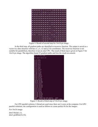
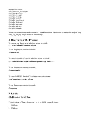
In the second step, to determine the new label of the center pixel in the neighborhood of 7x7
pixels; The label value with the maximum count within the Manhattan distance of 4 is selected as the
label of the center pixel. There are 37 pixes in this Manhattan distance if the pixel is at the middle of
image. If the maximum count value is less than 9 (~25% of 37), the label of the center pixel will be
labeled with 0. By using the 16x16 image experiment, for example, lets calculate the the labels of
[3,3]:
0 0 0 0 0 -> 5 pieces
1 -> 1 pieces
2 2 2 2 2 -> 5 pieces
3 3 3 3 3 3 3 -> 7 pieces
4 4 4 4 4 4 4 4 -> 8 pieces
5 5 5 5 5 5 -> 6 pieces
6 6 6 -> 3 pieces
7 -> 1 pieces
8 -> 1 pieces
At most, there are label 4 among 37 pixels. However [3,3] = 0 beause total count of label 4 is less than
25%.
The first and second steps are done using different matrixes for results. Because it is run on
parallel approach therefore we can not wait for convolution of pixels. We used initial matrix to
calculate the neighborhood and save the result into another matrix. We used 1-D (1 dimensional)
approach to hold the matrixes in array structes. In this structure, we can hold whole rows and cols in
only 1 dimension. This made the solution available for GPU, therefore we can not copy 2-D arrays
from host to device in CUDA. We copied 1-D arrays easily. The first step can be run on parallel.The
second step can be run on parallel too. However second step must wait until the first step is finished.
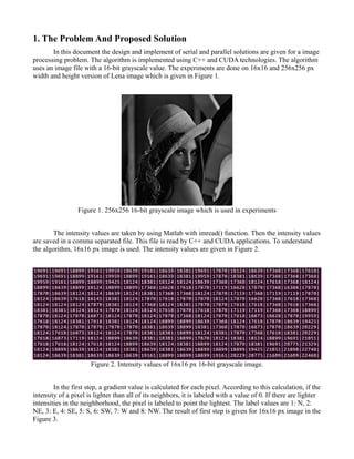
The result of second step is given in Figure 4.](https://image.slidesharecdn.com/sevalcaprazprojectreport-200507122712/85/Comparison-of-Parallel-Algorithms-For-An-Image-Processing-Problem-on-Cuda-3-320.jpg)
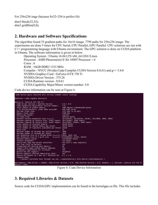
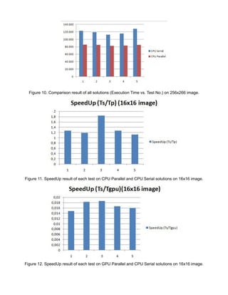
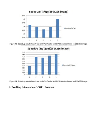

The document reports on a term project to design and implement serial and parallel solutions for an image processing algorithm. Experiments were conducted on 16x16 and 256x256 pixel images using C++ and CUDA. The CPU parallel solution was nearly 3 times faster than the GPU solution due to significant data transfer times between the CPU and GPU. While GPUs can provide massive parallelism, data transfers negated performance gains for this algorithm.