Comparative of Delay Tolerant Network Routings and Scheduling using Max-Weight, Back Pressure and ACO

International Journal on Recent and Innovation Trends in Computing and Communication ISSN: 2321-8169
Volume: 6 Issue: 7 78 - 85
______________________________________________________________________________________
78
IJRITCC | July 2018, Available @ http://www.ijritcc.org
______________________________________________________________________________________
Comparative of Delay Tolerant Network Routings and Scheduling using Max-
Weight, Back Pressure and ACO
1
S.Sindhupiriyaa, 2
Dr.D.Maruthanayagam
1
Research Scholar, Sri Vijay Vidyalaya College of Arts & Science, Dharmapuri, Tamilnadu.India.
2
Head cum Professor, PG and Research Department of Computer Science,
Sri Vijay Vidyalaya College of Arts & Science, Dharmapuri,Tamilnadu,India.
Abstract: Network management and Routing is supportively done by performing with the nodes, due to infrastructure-less nature of the
network in Ad hoc networks or MANET. The nodes are maintained itself from the functioning of the network, for that reason the MANET
security challenges several defects. Routing process and Scheduling is a significant idea to enhance the security in MANET. Other than,
scheduling has been recognized to be a key issue for implementing throughput/capacity optimization in Ad hoc networks. Designed underneath
conventional (LT) light tailed assumptions, traffic fundamentally faces Heavy-tailed (HT) assumption of the validity of scheduling algorithms.
Scheduling policies are utilized for communication networks such as Max-Weight, backpressure and ACO, which are provably throughput
optimality and the Pareto frontier of the feasible throughput region under maximal throughput vector. In wireless ad-hoc network, the issue of
routing and optimal scheduling performs with time varying channel reliability and multiple traffic streams. Depending upon the security issues
within MANETs in this paper presents a comparative analysis of existing scheduling policies based on their performance to progress the delay
performance in most scenarios. The security issues of MANETs considered from this paper presents a relative analysis of existing scheduling
policies depend on their performance to progress the delay performance in most developments.
Keywords: Mobile Ad hoc Networks, Heavy Tiled, Max-Weight, ACO, Backpressure, Delay Constrains.
__________________________________________________*****_________________________________________________
I. INTRODUCTION
Nowadays several military networks comprise wireless nodes that
exchange data without any support of external infrastructure such a
backbone wired network. In Mobile Ad-hoc Networks (MANETs),
it affords the desired qualities of flexibility and robustness required
for the unpredictable situations that occurs after taking out tactical
missions. For improving their performance of MANETs has
garnered a big deal of research aimed the rise in current usage. The
accessible physical resources and routing packets are scheduled
with the crucial elements affecting this performance. One of the
most fruitful and active fields of research in recent years, the area
of control of communication networks that includes several forms
of control, like routing process, scheduling performance, power
control, and congestion control. Queue length based scheduling
policies are well-known to be throughput optimal in a general
queuing network, like backpressure [7], max-weight scheduling
[6], ACO and its many variants. Consequently, back-Pressure
routing policies are guaranteed to stabilize a queuing network,
whenever possible. Scheduling policies of the max-weight family
has received more attention in different networking contexts,
including switches [8], satellites [9], wireless [10], and optical
networks [11]. Both the Tassiulas and Ephremides are presented
the Max-Weight scheduling in that such review.
The nature of instability of wireless routes and links, if it is check
whether due to fading, mobility or interference, gives for an
argument process. After that the physical layer resource allocation
must be jointly considered for performing operations of the rest of
the network protocol stack along with the flow-control, routing etc.
In cross-layer manages where network control policies compose
the resource scheduling and higher-layer routing depend on
physical layer parameters shown as big interest, the stability region
termed as throughput optimal algorithms [1, 2, 3]. A fundamental
limit affords to this region for utilizing network performance. The
stability region is the set of arrival rates for given that some
network control policy that it become stable the total queues in the
network exists, after those performing practical networks with
stochastic traffic.
II. SCHEDULING ALGORITHMS AND TECHNIQUES
1. Max-Weight Scheduling algorithm
A throughput-optimal scheduling policy-optimal scheduling policy
is concerned to the protocol model to activate a weighted
maximum independent set (WMIS) of the graph interference on
every time slot by referring about this author “Tassiulas and
Ephremides” [12]. The weight of a node is corresponding to the
queue length of the wireless link. It is also known as the maximum
weight scheduling (MWS) policy. As the Max-Weight algorithm
was initially defined, it has been revised in a variety of wire line
contexts and wireless links. A wide range of circumstances
performs for its popularity over the networks with throughput-
optimality. Throughput optimality means that it can serve each and
every one the offered packets and maintain the stability in feasible
manner.

______________________________________________________________________________________
79
______________________________________________________________________________________
In the special case of an ON/OFF downlink, the max-
weight rule is also called the Longest Connected Queue (LCQ)
scheduling rule. For example, the input-queued switch respect to
crossbar architecture is explained using below diagram. Consider
the N × N crossbar Input Queued (IQ) switch shown in figure 1,
there is N separate Virtual Output Queues (VOQ) at each of the
inputs that has equal to each of the N outputs. For output j of a
VOQ at input i is represented d by VOQij . Let Qij(t) signify the
number of packets in VOQij at time t. Consider at any time t, the
bipartite graph induced by performing with N inputs-outputs,
where an input i has an edge to output j if Qij(t) > 0. At every time
slot t needs the crossbar constraints of an IQ switch, an input know
how to be connected to at the majority of one output and each
output be able to receive at the majority of one packet from inputs.
An input-output is a “matching” on this bipartite graph which
means a feasible “schedule”. A matching of input-output be
capable of representing as a permutation matrix 𝜋 = (𝜋 ij) i,j ≤ N : 𝜋
ij = 1 if input i is matched to output j in the matching. A matching
or scheduling algorithm S attains a permutation (matching) 𝜋 S
(n)
for every time slot t. Weight of a VOQ refers regularly, but no
restriction to, the length (number of packets in backlog) of the
VOQ. Weight of the schedule is the sum of the weight of all the
VOQs which have been scheduled (matched) to the outputs in that
same time slot. That is, if 𝜋 = [𝜋 ij] is a schedule and Q(t) = [Qij(t)]
is the switch state at time t, after that the weight of schedule 𝜋 at
time t is ∑ijπ ijQij(t).
Figure1: Structure input-queued switch with crossbar
The scheduling algorithm searches the well-known maximum
weight matching (MWM) with maximum weight compare among
all possible N! Matching’s, to deliver 100% of throughput utilizes
MWM for admissible traffic.
Max-Weight scheduling algorithm with the aim of
support any 𝜆 such that (1 + 𝜖) 𝜆 𝜖 C. The Max-Weight scheduling
algorithm relates a weight q(h)
ij with the link equivalent to VOQ(i,
j) in the bipartite graph representation of the switch. After that, it
discovers a matching and the sum of the weights of the links
included in the matching; for this reason the name Max-Weight
algorithm.
The switch discovers a matching M(t) such that,
𝑀 𝑡 𝜖 arg max 𝑀(ℎ) ∑ 𝑞𝑖𝑗 𝑡 𝑀𝑖𝑗
(ℎ)
𝑖𝑗 ,
And transfers a packet from VOQ(i, j) to output port j if Mij(t) = 1
and qij(t) + aij(t) > 0, i.e., here is in the queue of a packet.
Queue length qij(t) preserves thought as the weight connected with
edge (i, j) in the complete bipartite graph representing the switch.
As a result, the Max-Weight algorithm discovers a matching with
the maximum sum weight among all matching’s, so is known as
Max-Weight scheduling.
Algorithm:
For each time slot
S ← ∅
for each layer from top to bottom
while (true)
n ← maximum weighted schedulable node
if n is NULL then break
Add n to S
End while
End for
Transmit packets from all nodes in S
End for
2. Back Pressure Algorithm
In this Backpressure routing, it has an essential algorithm for
dynamically a multi-hop network under routing traffic by utilizing
congestion gradients. The fundamental proposal of backpressure
scheduling [13] is able to choose the “best” set of non-interfering
links for transmission at each slot. Backpressure algorithm
includes sensor networks, heterogeneous networks and mobile ad
hoc networks (MANETS) with wireless component and wire-line
component, which applies into wireless communication networks.
The original backpressure algorithm was introduced by Tassiulas
and Ephremides. Two stages consist of a max-weight link selection
stage and a differential backlog routing stage. Backpressure
algorithm considers a multi-hop packet radio network with a fixed
set of link selection options and random packet arrivals.
Backpressure routing is intended to make decisions that minimize
the sum of squares of queue backlogs in the network from one
timeslot to the next slot, during the slotted time and it has been
unified with utility optimization techniques. Each and every
timeslot seeks to route data in directions that maximize the
differential backlog between neighboring nodes. This is
comparable to how water flows through a network of pipes through
pressure gradients. The Tassiulas-Ephremides algorithm was
initially called as "backpressure". The term "backpressure" has
derived a different meaning in the area of data networks.
Backpressure techniques utilize to provide high-priority
transmissions and the highest queue differentials over network
links. The packets flows through the network via pulled by gravity
towards the destination place and that it has the smallest queue size
of 0. Backpressure knows how to completely develop the available
network resources in an effective manner and a highly dynamic
Input
1
Input
N
Switching fabric
Matching M
Scheduler
Output 1
Output N
1
N
1
N

______________________________________________________________________________________
80
______________________________________________________________________________________
manner. Under low traffic conditions, on the other hand, since
many other nodes can also have a small or 0 queue sizes. Presently,
the process is inefficiency in terms of improving in delay, as
packets can take or loop a protracted time to arrive on the way to
the destination side.
An overview of the mathematical operation of the back-pressure
(BP) algorithm presents in this paper [24]. The time slot t denotes
with t th
time slot. The network represents using a graph G = (N,
L), where N corresponds to the group of nodes in the network and
L being the collection of links. Represent μ(n1,n2) [t] to be the
transmission rate (measured in packets/time-slot) of link (n1, n2) €
L between n1, n2 € N at time t, and 𝜇[t] = {μ(n1,n2) [t], (n1, n2) €
L}. At last Γ is the convex hull of the collection of all feasible
transmission rates in the network. Survey that 𝜇[t] and Γ could
based on the interference model used for performing with the
network. Let f[s,d] signify the flow from s to d. F represents the set
of all flows. Let x[s,d] be the rate in which s produces data for d,
and let 𝑥 = {x[s,d], [s, d] € F}. Allow C represents the capacity
region of the network under Γ. Each and every node in the network
preserves a queue for performing every other node in the network.
Let qj
i [t] denote the length of queue for node j maintained at node
i; the queue for node i maintained at i is assumed to be zero for all
time slots, i.e. qi
i [t] = 0 ∀t. In each time slot t, each node n
obtains queue information from its neighbor m ((n,m) € L). Define
𝑝(𝑛,𝑚)
𝑗
𝑡 = 𝑞 𝑛
𝑗
𝑡 -𝑞 𝑚
𝑗
𝑡 . Let
𝑗 𝑛,𝑚 [t]=arg max𝑗 𝑝(𝑛,𝑚)
𝑗
𝑡 . …………………………… (1)
In each time slot t, the network compute (1) and 𝜇[t] such that
𝜇[t] = arg 𝑚𝑎𝑥 𝜇∈𝛤{ ∑ 𝜇 𝑚,,𝑛𝑛.𝑚 𝜖𝑙 𝑝(𝑚,𝑛)
𝑗(𝑚,𝑛)[𝑡]
[t] } ……. (2)
Subsequent to finish the computation process, node m sent μ(m,n)[t]
packets out of queue j(m,n)[t] to node n in time slot t. Remind that
the maximization problem (sometimes known as the Max-Weight
problem) eq. (2) can be resolved in a distributed way for a wired
network. But, is a global issue for wireless networks because of the
coupled interference constraint and for that reason, it is an NP-hard
problem. The above scheduling algorithm and routing is confirm
and proven to be throughput optimality [14]; i.e. all queues in the
network were stabilized using BP if at all possible to do so under
any algorithm, and the capacity region under BP is the largest
possible. Several extensions are available for that great deal with
theoretically addressing both the distributed features in addition to
lowering the complexity [15, 16, 17].
Algorithm: backpressure at node i
1 for t=0,1,2,…do
2 observe local queue lengths {𝑞𝑖
𝑘
(t)}k for all
flows k
3 for all neighbors j ∈ ni do
4 send queue lengths {𝑞𝑖
𝑘
(t)}k – receive {𝑞𝑗
𝑘
(t)}k
5 determine flow with largest pressure:
6 𝑘𝑖𝑗
∗
= arg max 𝑘 [ 𝑞𝑖
𝑘
(t)-𝑞𝑗
𝑘
(t)]+
7 Set routing variables to 𝑟𝑖𝑗
𝑘
(t) = 0 for all k ≠ 𝑘𝑖𝑗
∗
and
8 𝑟𝑖𝑗
𝑘 𝑖𝑗
∗
(t) = 𝑐𝑖𝑗 Π {𝑞𝑖
𝑘 𝑖𝑗
∗
(t) - 𝑞𝑗
𝑘 𝑖𝑗
∗
(t) > 0 }
9 Transmit 𝑟𝑖𝑗
𝑘 𝑖𝑗
∗
(t) packets for flow 𝑘𝑖𝑗
∗
10 End
11 End
Example:
For case in point of the backpressure algorithm vigorously selects
the group of links to make active and flows to transmit on these
links based on queue backlogs and channel rates. Figure 2 show
how the backpressure algorithm works, if each of the nodes A, B,
C, and D form a three-hop wireless network that deals with two
flows. Each and every node has the same transmission rate but
cannot transmit as well as receive at the same time slot. In a
particular timeslot, the backlog of each node for each flow is
demonstrated in figure 2.
Figure 2: Example of the backpressure algorithm.
Backpressure algorithm works as given as follows. In the first
stage, the maximum differential queue backlog computes between
each node pair as a link weight; i.e., A→B is 5 for flow 1, C→B is
3 for flow 1, and D→C is 2 for flow 5, and choose these three
links. Secondly, list of all non-conflicting link sets, i.e., {A→B for
flow 1, D→C for flow 2} and {C→B for flow 1}.At last stage,
choose the set that maximizes the sum of all link weights, i.e.,
{A→B for flow 1, D→C for flow 5. At the present suppose node C
is malicious stage and declares that its queue backlog for flow 1 is
100.After that, the maximum differential queue backlog computes
between nodes B and C becomes 99 that makes backpressure
scheduling select only one link {C→B for flow 1}, thereby giving
the entire transmission opportunity to the malicious node C.
Figure 3: Information exchange and transmission scheduling
in the backpressure algorithm.
3. Ant Colony Optimization Algorithm
Ant colony optimization (ACO) algorithm is based on the Bio-
inspired algorithms; it has utilized to enhance the routing
algorithms for MANETs. Routing in MANETs is a challenging
because of MANETs dynamic features, its limited power energy
and bandwidth. ACO is particularly like a well-known swarm
Backlog information
exchange and channel
measurement
Scheduled transmissions
t-
1
t t
+
1
…
..
A B C D
6
2
1
3
4
5
5
7
5 3
2
Flow
1
Flow
2

______________________________________________________________________________________
81
______________________________________________________________________________________
intelligence approaches and it has acquired the inspiration from
real ants. In other case, they are wandering around their nests to
forage for searching the food [2]. In the lead of discovering food
they will return back to their nests at the same time as deposit
pheromone trails next to the paths, its next step depending on the
quantity of pheromone deposited on the path to the next node. The
ants may not handle anything except small control packets, which
have the task to search and gather whole information about it and a
path towards their destination. The main problem for searching
shortest paths maps rather than the issue of routing in networks.
Algorithm:
Input: An instance p of a ACO problem model p = (S,f,Ω)
intializePheromone Values(T)
S bs ← null
While termination conditions not met do
𝔖iter ← ∅
For j=1,…,na do
S ← Construct Solution (T)
If S is a valid solution then
S ← localsearch(S) {optional}
If (f(S) < f(S bs)) or (S bs = null) then S bs ← S
𝔖iter ← 𝔖iter ∪ { S }
End if
End for
Applypheromoneupdate(T, 𝔖iter, S bs )
End while
Output: the best so far solution S bs
The Ant Colony Optimization issues are generally modeled like a
graph. To prepare the ACO, the ants are represented as artificial
ants and that the paths are signified as edges of a graph G. A set of
basic components are C = c1, ..., cn. A solution of the issue
signifies by a subset S of components; the subset of feasible
solutions perform F ⊆ 2C
, therefore, if and only if S ∈ F that has a
solution S is feasible. The solution domain is defined under a cost
function f, f: 2C
→R, to discover a minimum cost feasible solution
S*, to find out S*: by using this formula S* ∈ ∀ F and f(S*) ≤
f(S), ∀ S ∈ F. A connected graph perform with n = V nodes and G
(V, E). Thus, these components cij are represented by either the
edges or the vertices of the graph. The objective of the problem is
to search a shortest path between the destination node Vd and the
source node Vs. Three equations are utilized for performing
simulates that the natural ant foraging process, Pheromone
evaporation, Pheromone increase, and Path selection. When an ant
current process, it performs at node i and transitions part handle to
node j:
𝜏 ij = 𝜏 ij + ∆𝜏
𝜏 ij is the artificial pheromone concentration over link j at i. The
artificial Pheromones progressively evaporate over time that has
modeled by:
𝜏 ij = (1 − 𝜆) * 𝜏 ij
Where (1−𝜆) is called the pheromone decrease constant. The ant
has to formulate a decision about the next level hop over in which
to travel at each node. The probability of an ant transitioning to
node j from node i at node d, where Ni signifies a set of neighbors,
is evaluated by the equation:
𝑝𝑖𝑗
𝑑
= { ( 𝜏𝑖𝑗
𝑘
/ ∑ 𝜏𝑖𝑗
𝑘
𝑗𝜖 𝑁𝑖
) if j ∈ Ni } and {d , otherwise.}
Where the route selection exponent denotes k and determines the
sensitivity of the ant algorithm to pheromone changes.
III. EXPERIMENTAL RESULTS:
With the intention of simulation process the max weight
scheduling algorithm and the backpressure for handling a
comprehensive simulation environment (Network Simulator-2).
The network simulator covers a huge number of applications of
multiple kinds of protocols of variable network types consisting of
variable network fundamentals and traffic model. For the
implementation process, both the stand alone the max weight
scheduling algorithm and backpressure algorithm, Network
Simulator (NS-2) is most well-liked simulation software and it is a
separate event packet level simulator. To imitate performance of
network simulator is a complete wrap up of tools like creating
network topologies, log events that takes place under any load to
examine the events and comprehend the network. NS-2 was and
preserved by USC and developed by UC Berkeley. In scientific
environment, network simulator is one of the most popular
simulators and it is based on the two languages such as OTcl and
C++. OTcl is defined an object oriented version of Tool Command
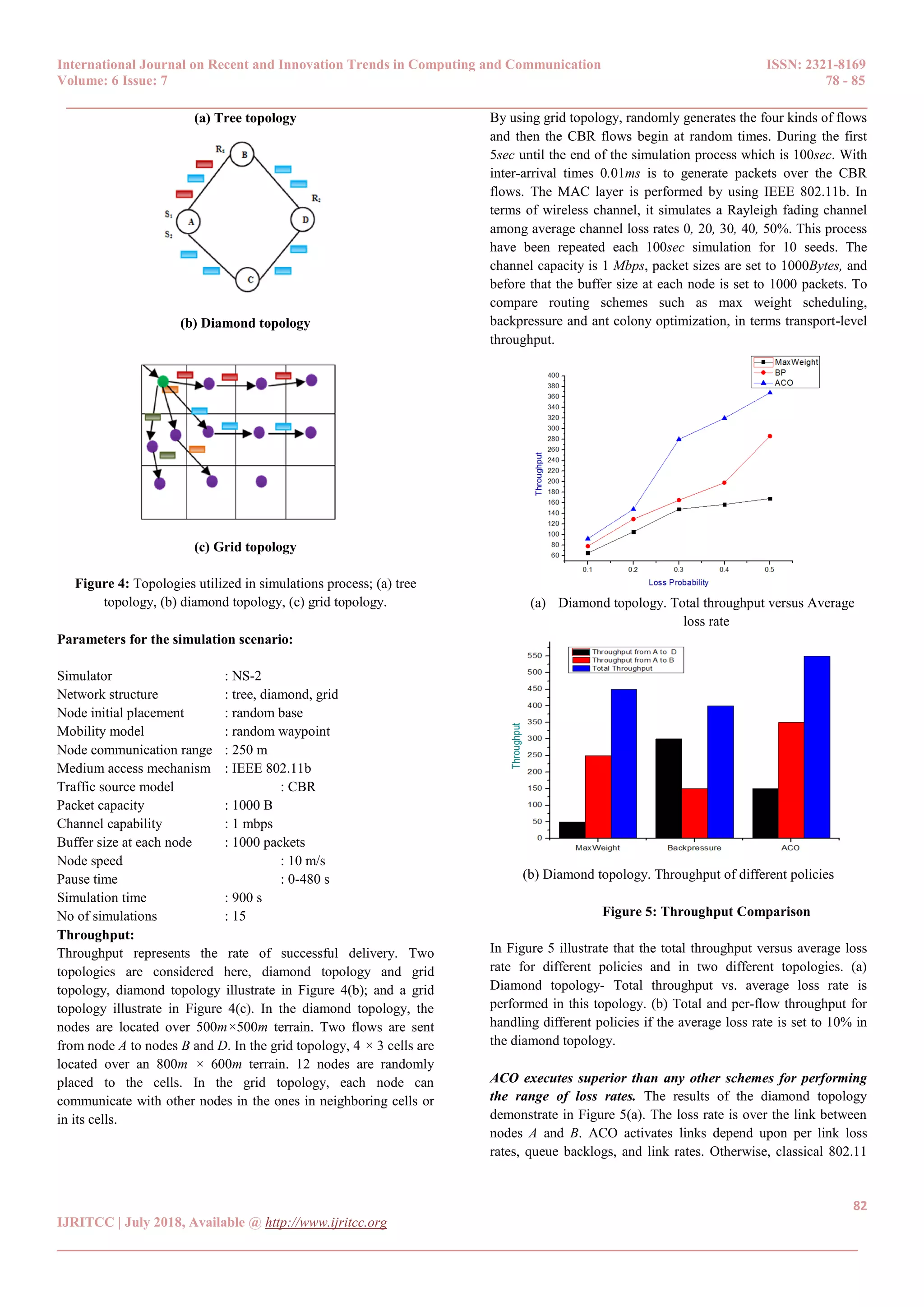
language. In simulation process, it considers three topologies such
as a tree topology, a diamond topology, and a grid topology
shown as follows Figure 4. These nodes are located over 500m ×
500m terrain and it denotes S1, S2 and R1, R2 which are likely
source-receiver pairs in the tree and diamond topologies.
The tree topology of S1 representation is initiated from node A and
ends on node B, and S2 representation is initiated from node A and
ends on node D. Within the diamond topology, it consists of two
flows between sources and receivers, S1, S2 and R1, R2,
respectively. S1 representation is initiated at node A and ends on
node B, and S2 representation is originated at node A and ends with
node D. Comparison of both topologies, all nodes are capable of
relaying packets to their neighbors. During the grid topology, 4× 3
cells are located over an 800m× 600m terrain. A gateway is
connected to the Internet and it passes flows to nodes. Each node
communicates with other nodes in its cell or neighboring cells, and
there are 12 nodes randomly placed to the cells.

______________________________________________________________________________________
82
______________________________________________________________________________________
(a) Tree topology
(b) Diamond topology
(c) Grid topology
Figure 4: Topologies utilized in simulations process; (a) tree
topology, (b) diamond topology, (c) grid topology.
Parameters for the simulation scenario:
Simulator : NS-2
Network structure : tree, diamond, grid
Node initial placement : random base
Mobility model : random waypoint
Node communication range : 250 m
Medium access mechanism : IEEE 802.11b
Traffic source model : CBR
Packet capacity : 1000 B
Channel capability : 1 mbps
Buffer size at each node : 1000 packets
Node speed : 10 m/s
Pause time : 0-480 s
Simulation time : 900 s
No of simulations : 15
Throughput:
Throughput represents the rate of successful delivery. Two
topologies are considered here, diamond topology and grid
topology, diamond topology illustrate in Figure 4(b); and a grid
topology illustrate in Figure 4(c). In the diamond topology, the
nodes are located over 500m×500m terrain. Two flows are sent
from node A to nodes B and D. In the grid topology, 4 × 3 cells are
located over an 800m × 600m terrain. 12 nodes are randomly
placed to the cells. In the grid topology, each node can
communicate with other nodes in the ones in neighboring cells or
in its cells.
By using grid topology, randomly generates the four kinds of flows
and then the CBR flows begin at random times. During the first
5sec until the end of the simulation process which is 100sec. With
inter-arrival times 0.01ms is to generate packets over the CBR
flows. The MAC layer is performed by using IEEE 802.11b. In
terms of wireless channel, it simulates a Rayleigh fading channel
among average channel loss rates 0, 20, 30, 40, 50%. This process
have been repeated each 100sec simulation for 10 seeds. The
channel capacity is 1 Mbps, packet sizes are set to 1000Bytes, and
before that the buffer size at each node is set to 1000 packets. To
compare routing schemes such as max weight scheduling,
backpressure and ant colony optimization, in terms transport-level
throughput.
(a) Diamond topology. Total throughput versus Average
loss rate
(b) Diamond topology. Throughput of different policies
Figure 5: Throughput Comparison
In Figure 5 illustrate that the total throughput versus average loss
rate for different policies and in two different topologies. (a)
Diamond topology- Total throughput vs. average loss rate is
performed in this topology. (b) Total and per-flow throughput for
handling different policies if the average loss rate is set to 10% in
the diamond topology.
ACO executes superior than any other schemes for performing
the range of loss rates. The results of the diamond topology
demonstrate in Figure 5(a). The loss rate is over the link between
nodes A and B. ACO activates links depend upon per link loss
rates, queue backlogs, and link rates. Otherwise, classical 802.11

______________________________________________________________________________________
83
______________________________________________________________________________________
MAC utilizes by Backpressure and Max-Weight, which presents
fairness among the competing nodes for the medium, which is not
utility optimal. If the loss rate over link A − B enhances, the total
throughput of all the schemes minimizes as expected.
The throughput of two flows A to D and A to B and their total
value in figure 5(b), if the loss rate is over 10% link A−B. Consider
Figure 5(a) again. Backpressure and Max-Weight improve
throughput majorly as compared to other routing schemes to
explore the new routes to develop utility (throughput). In this
topology, over other routing schemes is up to 22% and also
Backpressure and Max-Weight have similar throughput
performance, which emphasis the advantage of routing part and the
efficient link layer queue estimation mechanism of Backpressure.
The throughput improvement of all schemes are similar due to loss
rate is 50% in Fig. 5(a), link A − B develops into very inefficient,
after that all of the schemes sent packets mostly from flow A to D
over path A − C − D and have related performance at high loss
rates.
As results of the grid topology illustrate in figure 5(b). The
throughput improvement of Max-Weight is higher than other
schemes for all loss rates in the grid topology and higher as
compared to the improvement in the diamond topology, for
instance, the improvement is up to 33% in the grid topology. For
that reason is the existing routing that has designed to discover the
shortest paths, however, Max-Weight schemes are capable to
explore interference free paths, if they are not the shortest paths
and it is emphasized in larger topologies. ACO algorithm
successfully increases the throughput rate compared with other
algorithms (BP and Max-Weight).
Packet Delivery Ratio:
The packet delivery ratio is the ratio of the total set of the packets
effectively received using the destination nodes to transmit set of
packets by source nodes on the way to throughout the simulation.
As the results of a long time simulation and short time simulation
are performed up to 3 and 12 hours in figure 6. In that figure
simulates the backpressure routing protocol and the energy version
of the familiar protocols. As of the results know how to conclude
that the performance of Max-Weight, backpressure algorithm and
ACO have the most excellent results. A simulation of both
protocols (backpressure and Max-Weight and ACO with 10
replicas) in Figure 6. The results the long simulation has a better
delivery ratio, and finally concludes that Backpressure protocol has
superior improvement in energy consumption compared to Max-
Weight and ACO, at the same time as sustaining the delivery ratio.
A well known challenge to backpressure routing algorithms
perform in Packet delivery latency. ACO algorithm majorly
increases the delivery ratio of emergency packets compared with
other algorithms (BP and Max-Weight).
Figure 6: Delivery ratio and average remaining energy in 3-
and 12-hour
Average delay:
Figure 7: Performance of BP, MWS, and ACO in a linear
network topology (𝝐 = 0.005).
By measuring average packet delays to evaluate the performance
(in unit of time slot) over all the delivered packets (arrive at their
respective destination nodes) in the network. The average delays
under different offered loads to examine the performance limits of
different scheduling schemes plots at Figure 7. As result of
simulation run that lasts for 107
time slots. In view of the fact that
the optimal throughput region Λ*
is described as the set of arrival
rate vectors under that queue lengths and thus delays remain finite,
consider the traffic load under that the average delay increases
quickly, as the boundary of the optimal throughput region. Fig. 7
shows that all schemes achieve the same boundary (i.e., λ < 0.5)
which supports results on throughput optimality. Also, the Max-
Weight schemes achieve substantially better delay performance
than the back-pressure algorithm. This is because under the back-
pressure algorithm, the queue lengths have to build up along the

______________________________________________________________________________________
84
______________________________________________________________________________________
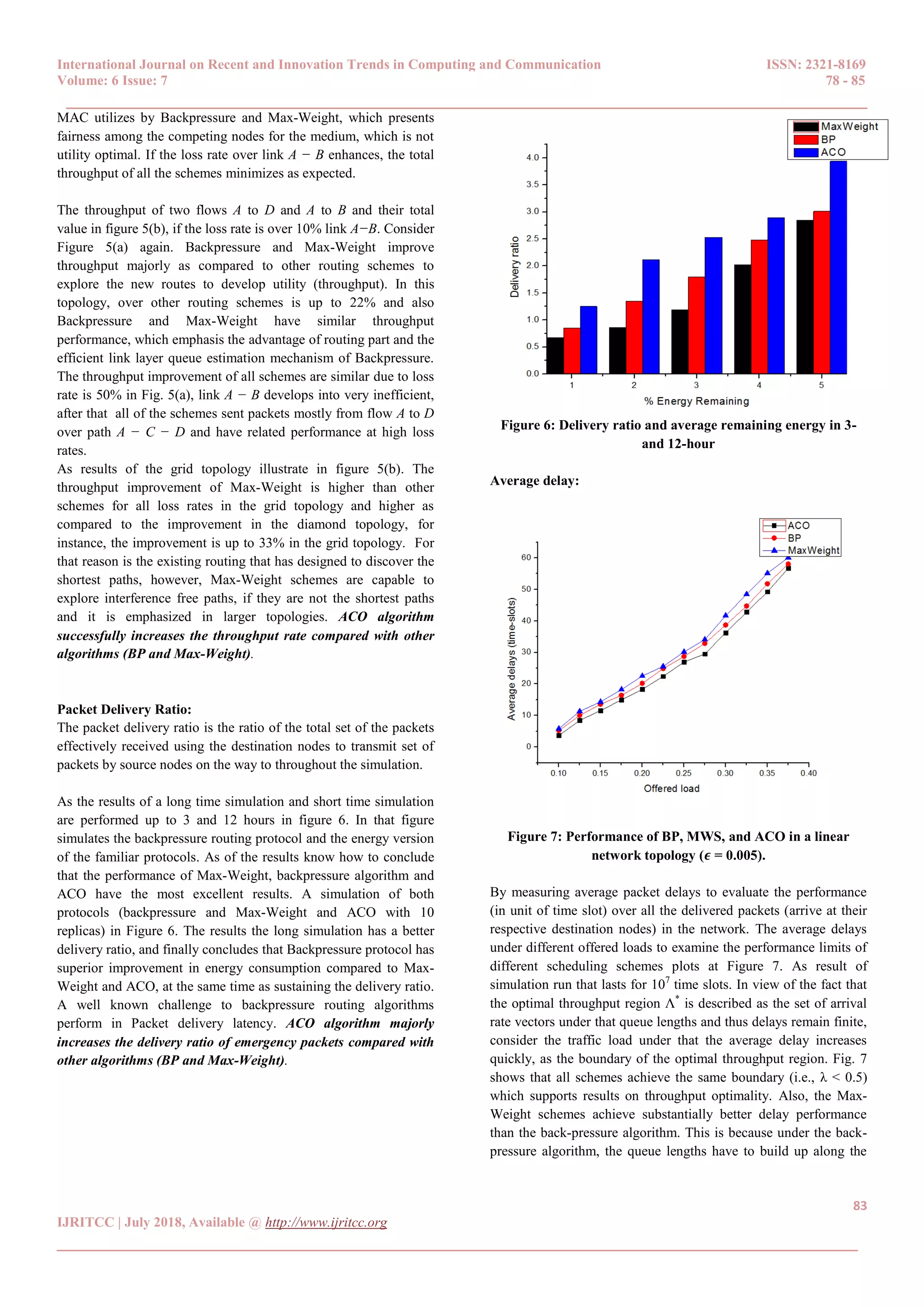
route a flow takes from the destination to the source, and in
general, earlier hop link has a larger queue length. This leads to
poor delay performance especially when the route of a flow is
lengthy. ACO algorithm reduces the average delay for packets
compared with other algorithms (BP and Max-Weight).
End-to-end delay:
The end-to-end delay of a packet is described as the number of
time-slots it spends in the system earlier than arrive at the intended
user. This comprises the time-slot at the beginning of which the
packet arrival at the base station. End-to-end delay performance of
three algorithms is compared with the Backpressure, Max-Weight
and ACO.
Figure 8: End-to-end delay of emergency packets.
End-to-end delay of emergency packets varies 𝜆 from 0.1 to 0.5
shown in Fig. 8. From the simulations know how to observe that:
1) If the network load is low, the backpressure queuing model is
high over the end-to-end delay of emergency packets. For the
reason that the queue backlog difference gradient is not
formed, and then the Backpressure survey with the all
possible routes. The backpressure queuing model is relatively
higher than the Max-Weight queuing model, as the queuing
model is modified into Max-Weight.
2) If the network load enhances, the backpressure queuing model
first reduces after that enhances over the end-to-end delay of
emergency packets. When the packets arrival rate is formed
0:2 in the queue backlog difference gradient, thus, the end-to-
end delay automatically reduces in an effective manner.
Subsequently, the end-to-end delay enhances the performance
due to the increasing of queue backlog. The end-to-end delay
of Max-Weight reduces for the reason that the formation of
queue backlog difference gradient, the later packets can be
delivered in a rapid manner. Hence, the delay reduces when
the packets arrival rate is larger than 0:5.
3) ACO based queuing model is smaller than that two queuing
model over the end-to-end delay of emergency packets, it has
the shortest waiting time in queue and priority to be
forwarded. ACO algorithm majorly reduces the end-to-end
delay compared with other algorithms (BP and Max-
Weight). In the real-time performance of emergency packets
know how to be protected and assured with the support of
ACO schemes.
IV. CONCLUSION
In MANET process, the majority issues of routing and optimal
scheduling handles by way of time varying channel reliability and
multiple traffic streams with the support of an ad-hoc network. A
trouble-free way to save packet delay time by using delay-based
scheduling that plagues its queue length based counterpart.
Subsequently, the waiting time reduces for performing emergency
packets in queues. The significant performance of existing
techniques is evaluated from this paper. Depending upon the
performance evaluation in the ACO algorithm is to develop
throughput majorly as compared to other routing schemes like
Backpressure and Max-Weight. For the reason that Backpressure
and Max-Weight algorithm leads to poor performance delay
particularly if the route of a flow is lengthy manner. The
experimental results explain that the ACO algorithm successfully
increases the throughput rate and majorly reduces the average
delay, end-to-end delay and increases the delivery ratio of
emergency packets compared with other traditional queuing model
algorithms.
REFERENCES
[1]. L. Georgiadis, M. J. Neely, and L. Tassiulas. Resource
Allocation and Cross-layer Control in Wireless
Networks. Foundations and Trends in Networking, 2006.
[2]. L. Tassiulas and A. Ephremides. Stability Properties of
Constrained Queuing Systems and Scheduling Properties
for Maximum Throughput in Multihop Radio Networks.
IEEE Transactions on Automatic Control, 37(12):1936–
1948, December 1992.
[3]. E. M. Yeh and R. A. Berry. Throughput Optimal Control
of Cooperative Relay Networks. IEEE Transcations on
Information Theory: Special Issue on Models, Theory,
and Codes for Relaying and Cooperation in
Communication Networks, 53(10):3827–3832, October
2007.
[4]. T. J. Oechtering and H. Boche. Stability Region of an
Efficient Bidirectional Regenerative Half-duplex
Relaying Protocol. In Proc. IEEE Information Theory
Workshop, 2006. ITW ’06, Chengdu, China, October
2006.
[5]. L. Tassiulas, A. Ephremides (1992). Stability properties
of constrained queueing systems and scheduling policies
for maximum throughput in multihop radio networks.
IEEE Transactions on Automatic Control, 37, 1936-
1948.
[6]. B. Ji, C. Joo, N.B. Shro_ (2013). Throughput-optimal
scheduling in multihop wireless networks without per-
ow information. IEEE/ACM Transactions on
Networking, 21(2), pp. 634-647.

______________________________________________________________________________________
85
______________________________________________________________________________________
[7]. B. Ji, C. Joo, N.B. Shro_ (2013). Delay-based Back-
Pressure scheduling in multihop wireless networks.
IEEE/ACM Transactions on Networking, 21(5), pp.
1539-1552.
[8]. A. Ganti, E. Modiano, J.N. Tsitsiklis (2007). Optimal
transmission scheduling in symmetric communication
models with intermittent connectivity. IEEE
Transactions on Information Theory, 53(3), pp. 998-
1008.
[9]. L. Georgiadis, M. Neely, L. Tassiulas (2006). Resource
allocation and cross-layer control in wireless networks.
Foundations and Trends in Networking, 1(1), pp. 1-144.
[10]. A. Gut (2005). Probability: a Graduate Course. Springer
Texts in Statistics, Springer-Verlag.
[11]. O. Boxma, B. Zwart (2007). Tails in scheduling.
Performance Evaluation Review, 34(4), 13-20.
[12]. L. Tassiulas and A. Ephremides, “Stability properties of
constrained queueing systems and scheduling policies
for maximum throughput in multihop radio networks,”
IEEE Transactions on Automatic Control, vol. 37, no.
12, pp. 1936–1948, Dec 1992.
[13]. L. Bui, R. Srikant, and A. L. Stolyar. A novel
architecture for delay in the back-pressure scheduling
algorithm. IEEE/ACM Trans. Networking. Submitted,
2009.
[14]. L. Tassiulas and A. Ephremides. Stability properties of
constrained queuing systems and scheduling for
maximum throughput in multi-hop radio networks. IEEE
Transactions on Automatic Control, 37(12):1936–1949,
December 1992.
[15]. U. Akyol, M. Andrews, P. Gupta, J. Hobby, I. Saniee,
and A. Stolyar. Joint scheduling and congestion control
in mobile ad-hoc networks. In IEEE Infocom, 2008.
[16]. L. Bui, R. Srikant, and A. Stolyar. Novel architectures
and algorithms for delay reduction in back-pressure
scheduling and routing. In Proc. of IEEE INFOCOM
Mini-Conference, 2009.
[17]. L. Ying, R. Srikant, and D. Towsley. Cluster-based
back-pressure routing algorithm. In Proceedings of IEEE
INFOCOM, 2008.
ABOUT THE AUTHORS
B. Sindhupiriyaa received her M.Phil Degree
from Periyar University, Salem in the year
2015. She has received her M.C.A Degree
from Anna University,Coimbatore in the the
year 2011. She is pursuing her Ph.D Degree at
Sri Vijay Vidyalaya College of Arts & Science
(Affiliated Periyar University),Dharmapuri,
Tamilnadu, India. Her areas of interest include Mobile Computing
and Wireless Networking.
Dr. D. Maruthanayagam received his Ph.D
Degree from Manonmaniam Sundaranar
University,Tirunelveli in the year 2014. He
received his M.Phil Degree from
Bharathidasan University, Trichy in the year
2005. He received his M.C.A Degree from
Madras University, Chennai in the year 2000.
He is working as HOD Cum Professor, PG and Research
Department of Computer Science, Sri Vijay Vidyalaya College of
Arts & Science, Dharmapuri, Tamilnadu, India. He has above 15
years of experience in academic field. He has published 4 books,
27 papers in International Journals and 28 papers in National &
International Conferences so far. His areas of interest include
Computer Networks, Grid Computing, Cloud Computing and
Mobile Computing.

Comparative of Delay Tolerant Network Routings and Scheduling using Max-Weight, Back Pressure and ACO

Recommended

Recommended

More Related Content

What's hot

What's hot (18)

Similar to Comparative of Delay Tolerant Network Routings and Scheduling using Max-Weight, Back Pressure and ACO

Similar to Comparative of Delay Tolerant Network Routings and Scheduling using Max-Weight, Back Pressure and ACO (20)

More from rahulmonikasharma

More from rahulmonikasharma (20)

Recently uploaded

Recently uploaded (20)

Comparative of Delay Tolerant Network Routings and Scheduling using Max-Weight, Back Pressure and ACO