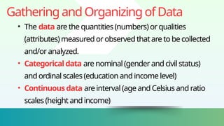
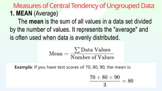
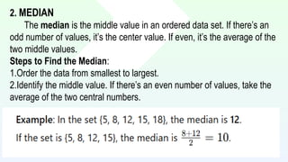
2. MEDIAN
The medianis the middle value in an ordered data set. If there’s an
odd number of values, it’s the center value. If even, it’s the average of the
two middle values.
Steps to Find the Median:
1.Order the data from smallest to largest.
2.Identify the middle value. If there’s an even number of values, take the
average of the two central numbers.
15.
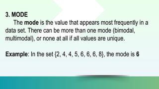
3. MODE
The modeis the value that appears most frequently in a
data set. There can be more than one mode (bimodal,
multimodal), or none at all if all values are unique.
Example: In the set {2, 4, 4, 5, 6, 6, 6, 8}, the mode is 6
16.
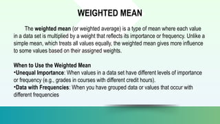
WEIGHTED MEAN
The weightedmean (or weighted average) is a type of mean where each value
in a data set is multiplied by a weight that reflects its importance or frequency. Unlike a
simple mean, which treats all values equally, the weighted mean gives more influence
to some values based on their assigned weights.
When to Use the Weighted Mean
•Unequal Importance: When values in a data set have different levels of importance
or frequency (e.g., grades in courses with different credit hours).
•Data with Frequencies: When you have grouped data or values that occur with
different frequencies
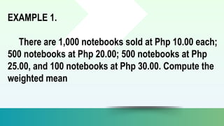
EXAMPLE 1.
There are1,000 notebooks sold at Php 10.00 each;
500 notebooks at Php 20.00; 500 notebooks at Php
25.00, and 100 notebooks at Php 30.00. Compute the
weighted mean
19.
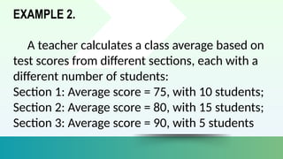
EXAMPLE 2.
A teachercalculates a class average based on
test scores from different sections, each with a
different number of students:
Section 1: Average score = 75, with 10 students;
Section 2: Average score = 80, with 15 students;
Section 3: Average score = 90, with 5 students
20.
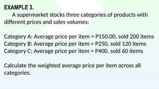
EXAMPLE 3.
A supermarketstocks three categories of products with
different prices and sales volumes:
Category A: Average price per item = P150.00, sold 200 items
Category B: Average price per item = P250, sold 120 items
Category C: Average price per item = P400, sold 60 items
Calculate the weighted average price per item across all
categories.
21.
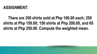
ASSIGNMENT:
There are 350shirts sold at Php 100.00 each; 250
shirts at Php 150.00; 150 shirts at Php 200.00, and 65
shirts at Php 250.00. Compute the weighted mean.
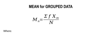
Steps to findthe mean of grouped data:
1. Find the class mark for each class interval:
𝑋𝑚=
𝐿𝑜𝑤𝑒𝑟 𝐿𝑖𝑚𝑖𝑡+𝑈𝑝𝑝𝑒𝑟 𝐿𝑖𝑚𝑖𝑡
2
2. Multiply each class mark by the class frequency:
3. Find the
4. Sum up all frequencies:
5. Divide: by togetthemean.
24.
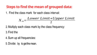
EXAMPLE 1.
The tablebelow summarizes the weights of goats. Find the
average weight of the goats.
WEIGHT OF GOATS
201 – 210 3
191 – 200 8
181 – 190 12
171 – 180 11
161 – 170 9
151 – 160 2
25.
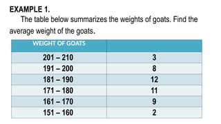
EXAMPLE 2.
The tablebelow shows the distribution of workers’ ages:
WORKERS’ AGES
21 – 30 7
31 – 40 8
41 – 50 5
51 – 60 3
61 – 70 2
26.
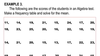
EXAMPLE 3.
The followingare the scores of the students in an Algebra test.
Make a frequency table and solve for the mean.
11, 14, 19, 21, 15, 24, 17, 20,
18, 23, 25, 20, 16, 22, 18, 19,
14, 21, 20, 15, 13, 17, 22, 23,
27.
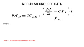
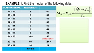
𝑀 𝑑 =𝑋 𝐿𝐵 +
( 𝑁
2
−𝑐𝑓 𝑏 )𝑖
𝑓 𝑚
MEDIAN for GROUPED DATA
Where:
NOTE: To determine the median class:
28.
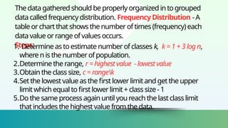
CLASS INTERVAL FREQUENCY
28– 29 1 60
26 – 27 3 59
24 – 25 3 56
22 – 23 3 53
20 – 21 6 50
18 – 19 6 44
16 – 17 8 38
14 – 15 6 = 30
median class
12 – 13 10 24 =
10 – 11 14 14
N = 60
EXAMPLE 1. Find the median of the following data:
𝑀𝑑= 𝑋𝐿𝐵 +
(𝑁
2
−𝑐𝑓 𝑏)𝑖
𝑓 𝑚
𝑀 𝑜= 𝑋𝐿𝐵+
[ 𝑑 𝑓 1
𝑑 𝑓 1 + 𝑑 𝑓 2
]𝑖
MODE for GROUPED DATA
Where:
NOTE: The modal class is the class with the highest frequency
31.
CLASS INTERVAL FREQUENCY
28– 29 1
26 – 27 3
24 – 25 3
22 – 23 3
20 – 21 6
18 – 19 6
16 – 17 8
14 – 15 6
12 – 13 10
10 – 11 14
modal class
N = 60
EXAMPLE 1. Find the mode of the following data:
𝑀𝑜= 𝑋 𝐿𝐵+
[ 𝑑 𝑓 1
𝑑 𝑓 1 +𝑑 𝑓 2
]𝑖
32.
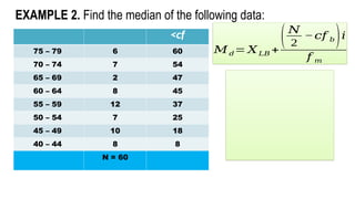
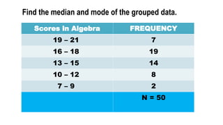
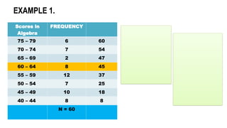
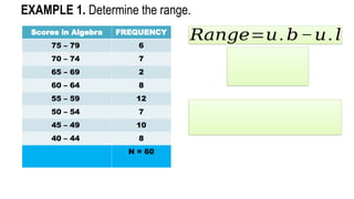
Scores in AlgebraFREQUENCY
75 – 79 6
70 – 74 7
65 – 69 2
60 – 64 8
55 – 59 12
50 – 54 7
45 – 49 10
40 – 44 8
N = 60
EXAMPLE 2. Find the mode of the following data:
𝑀𝑜= 𝑋 𝐿𝐵+
[ 𝑑 𝑓 1
𝑑 𝑓 1 +𝑑 𝑓 2
]𝑖
33.
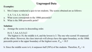
Scores in AlgebraFREQUENCY
19 – 21 7
16 – 18 19
13 – 15 14
10 – 12 8
7 – 9 2
N = 50
Find the median and mode of the grouped data.
34.
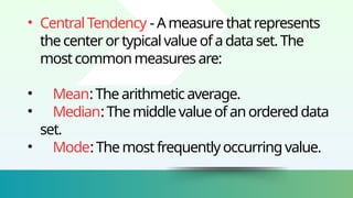
Measure of RelativePosition
The measure of relative position helps us understand
how a particular data point compares to the other
values in a dataset. Commonly used measures include
percentiles, quartiles and deciles. These measures
allow us to see how high or low a value is in relation to
the rest of the data.
35.
1. Percentiles
Percentiles areused to describe the position of a value
relative to the entire dataset. They tell you what
percentage of data values fall below a certain point.
•Definition:
•A percentile divides a dataset into 100 equal parts.
•Example: If you are at the 75th percentile, this means
you scored better than 75% of the people
36.
Ungrouped Data
Examples:
1. Mrs.Corpuzconducted a quiz to ten students. The scores obtained are as follows:
5, 8, 7, 6, 3, 6, 10,5,6,4
a. What score corresponds to the 100th percentile?
b. What is the 50th percentile point?
Solution:
c. Arrange the scores in descending order.
10, 8, 7, 6,6, 6,5,5,4,3
The highest is 10, the middle is 6, and the lowest is 3. The one who scored 10 surpassed
all the others. However, the class intervals will always have the upper boundary, so the 100th
percentile point is the upper boundary of the highest score. P100 = 10.5
b. Since the middle score is 6, it surpasses half (50%) of the students. Therefore, P50 = 6
37.
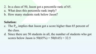
2. In aclass of 50, Jason got a percentile rank of 65.
a. What does this percentile rank imply?
b. How many students rank below Jason?
Solution:
c. The P65 implies that Jason got a score higher than 65 percent of
the class.
d. Since there are 50 students in all, the number of students who got
scores below Jason is 50(65%) = 50(0.65) = 32.5
38.
𝑃𝑛= 𝑋 𝐿𝐵+𝑖
[𝑛𝑁 − 𝐹
𝑓 ]
PERCENTILE for GROUPED DATA
Where:
NOTE: To determine the percentile class:
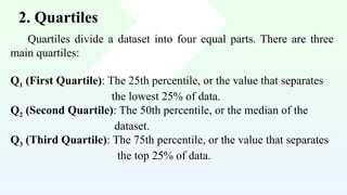
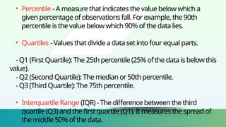
2. Quartiles
Quartiles dividea dataset into four equal parts. There are three
main quartiles:
Q1 (First Quartile): The 25th percentile, or the value that separates
the lowest 25% of data.
Q2 (Second Quartile): The 50th percentile, or the median of the
dataset.
Q3 (Third Quartile): The 75th percentile, or the value that separates
the top 25% of data.
42.
𝑄𝑛 = 𝑋𝐿𝐵+𝑖 [
𝑁
4
− 𝐹
𝑓 ]
QUARTILES for GROUPED DATA
Where:
NOTE: To determine the quartile class: ; ;
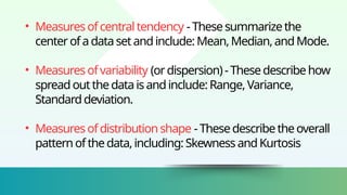
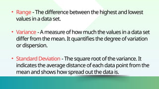
Measure of Variation
Measuresof variation describe the spread or dispersion
of a dataset. They indicate how much the data values
differ from each other or from the central tendency. The
key measures of variation include range, variance,
standard deviation, mean deviation, quartile
deviation and interquartile range (IQR).
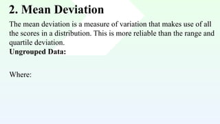
2. Mean Deviation
Themean deviation is a measure of variation that makes use of all
the scores in a distribution. This is more reliable than the range and
quartile deviation.
Ungrouped Data:
Where:
61.
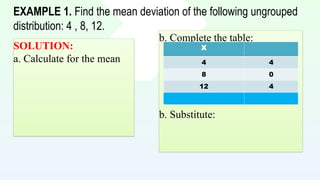
EXAMPLE 1. Findthe mean deviation of the following ungrouped
distribution: 4 , 8, 12.
SOLUTION:
a. Calculate for the mean
b. Complete the table:
b. Substitute:
X
4 4
8 0
12 4
62.
𝑴𝑫 =
∑ 𝒇|𝑿𝒎 − 𝑴 𝒏|
𝑵
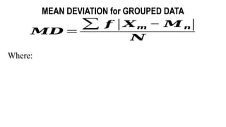
MEAN DEVIATION for GROUPED DATA
Where:
63.
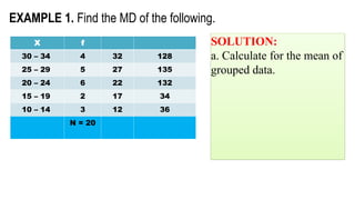
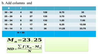
X f
30 –34 4 32 128
25 – 29 5 27 135
20 – 24 6 22 132
15 – 19 2 17 34
10 – 14 3 12 36
N = 20
EXAMPLE 1. Find the MD of the following.
SOLUTION:
a. Calculate for the mean of
grouped data.
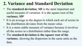
2. Variance andStandard Deviation
• The standard deviation, SD is the most important and
useful measure of variation. It is the square root of the
variance, SD2
• It is an average to the degree to which each set of scores in
the distribution deviates from the mean value.
• It is a more stable measure of variance because it involves
all the scores in a distribution rather than the range.
• The standard deviation is the square root of the
variance, showing the dispersion in the same units as the
data.
66.
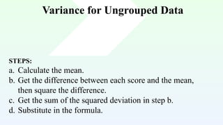
Variance for UngroupedData
STEPS:
a. Calculate the mean.
b. Get the difference between each score and the mean,
then square the difference.
c. Get the sum of the squared deviation in step b.
d. Substitute in the formula.
67.
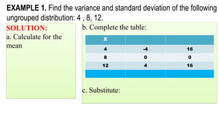
EXAMPLE 1. Findthe variance and standard deviation of the following
ungrouped distribution: 4 , 8, 12.
SOLUTION:
a. Calculate for the
mean
b. Complete the table:
c. Substitute:
X
4 -4 16
8 0 0
12 4 16
68.
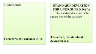
C. Substitute:
Therefore, thevariance is 16.
STANDARD DEVIATION
FOR UNGROUPED DATA
The standard deviation is the
square root of the variance
Therefore, the standard
deviation is 4.
69.
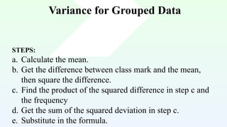
Variance for GroupedData
STEPS:
a. Calculate the mean.
b. Get the difference between class mark and the mean,
then square the difference.
c. Find the product of the squared difference in step c and
the frequency
d. Get the sum of the squared deviation in step c.
e. Substitute in the formula.
70.
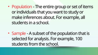
• Population -The entire grouporsetofitems
orindividuals thatyouwantto studyor
makeinferences about.For example,all
students ina school.
• Sample - Asubset ofthe populationthatis
selectedforanalysis.For example,100
students from the school.


![𝑀 𝑜= 𝑋 𝐿𝐵+
[ 𝑑 𝑓 1
𝑑 𝑓 1 + 𝑑 𝑓 2
]𝑖
MODE for GROUPED DATA
Where:
NOTE: The modal class is the class with the highest frequency](https://image.slidesharecdn.com/mmw-mathematics-as-a-tool-complete-250829134215-2e1becda/85/mathematics-as-a-tool-major-in-Elementary-Education-30-320.jpg)
![CLASS INTERVAL FREQUENCY
28 – 29 1
26 – 27 3
24 – 25 3
22 – 23 3
20 – 21 6
18 – 19 6
16 – 17 8
14 – 15 6
12 – 13 10
10 – 11 14
modal class
N = 60
EXAMPLE 1. Find the mode of the following data:
𝑀𝑜= 𝑋 𝐿𝐵+
[ 𝑑 𝑓 1
𝑑 𝑓 1 +𝑑 𝑓 2
]𝑖](https://image.slidesharecdn.com/mmw-mathematics-as-a-tool-complete-250829134215-2e1becda/85/mathematics-as-a-tool-major-in-Elementary-Education-31-320.jpg)
![Scores in Algebra FREQUENCY
75 – 79 6
70 – 74 7
65 – 69 2
60 – 64 8
55 – 59 12
50 – 54 7
45 – 49 10
40 – 44 8
N = 60
EXAMPLE 2. Find the mode of the following data:
𝑀𝑜= 𝑋 𝐿𝐵+
[ 𝑑 𝑓 1
𝑑 𝑓 1 +𝑑 𝑓 2
]𝑖](https://image.slidesharecdn.com/mmw-mathematics-as-a-tool-complete-250829134215-2e1becda/85/mathematics-as-a-tool-major-in-Elementary-Education-32-320.jpg)
![𝑃𝑛= 𝑋 𝐿𝐵 +𝑖
[𝑛𝑁 − 𝐹
𝑓 ]
PERCENTILE for GROUPED DATA
Where:
NOTE: To determine the percentile class:](https://image.slidesharecdn.com/mmw-mathematics-as-a-tool-complete-250829134215-2e1becda/85/mathematics-as-a-tool-major-in-Elementary-Education-38-320.jpg)
![CLASS INTERVAL FREQUENCY
28 – 29 1 60
26 – 27 3 59
24 – 25 3 56
22 – 23 3 53
20 – 21 6 50
18 – 19 6 44
16 – 17 8 38
14 – 15 6 30
12 – 13 10 24
10 – 11 14 14
N = 60
EXAMPLE 1. Find the
𝑃𝑛= 𝑋𝐿𝐵 +𝑖
[𝑛𝑁 − 𝐹
𝑓 ]](https://image.slidesharecdn.com/mmw-mathematics-as-a-tool-complete-250829134215-2e1becda/85/mathematics-as-a-tool-major-in-Elementary-Education-39-320.jpg)
![Scores in Algebra FREQUENCY
75 – 79 6
70 – 74 7
65 – 69 2
60 – 64 8
55 – 59 12
50 – 54 7
45 – 49 10
40 – 44 8
N = 60
EXAMPLE 2. Find the
𝑃𝑛= 𝑋𝐿𝐵 +𝑖
[𝑛𝑁 − 𝐹
𝑓 ]](https://image.slidesharecdn.com/mmw-mathematics-as-a-tool-complete-250829134215-2e1becda/85/mathematics-as-a-tool-major-in-Elementary-Education-40-320.jpg)
![𝑄𝑛 = 𝑋 𝐿𝐵+𝑖 [
𝑁
4
− 𝐹
𝑓 ]
QUARTILES for GROUPED DATA
Where:
NOTE: To determine the quartile class: ; ;](https://image.slidesharecdn.com/mmw-mathematics-as-a-tool-complete-250829134215-2e1becda/85/mathematics-as-a-tool-major-in-Elementary-Education-42-320.jpg)
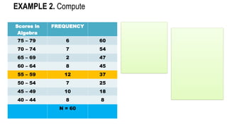
![Scores in
Algebra
FREQUENCY
75 – 79 6 60
70 – 74 7 54
65 – 69 2 47
60 – 64 8 45
55 – 59 12 37
50 – 54 7 25
45 – 49 10 18
40 – 44 8 8
N = 60
EXAMPLE 1. Compute
𝑄𝑛= 𝑋 𝐿𝐵+𝑖 [
𝑁
4
− 𝐹
𝑓 ]](https://image.slidesharecdn.com/mmw-mathematics-as-a-tool-complete-250829134215-2e1becda/85/mathematics-as-a-tool-major-in-Elementary-Education-43-320.jpg)

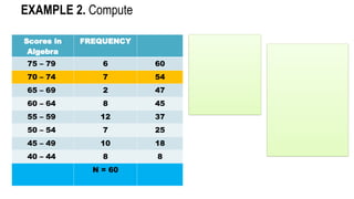
![Scores in
Algebra
FREQUENCY
75 – 79 6 60
70 – 74 7 54
65 – 69 2 47
60 – 64 8 45
55 – 59 12 37
50 – 54 7 25
45 – 49 10 18
40 – 44 8 8
N = 60
EXAMPLE 2. Compute
𝑄𝑛= 𝑋 𝐿𝐵+𝑖 [
𝑁
4
− 𝐹
𝑓 ]](https://image.slidesharecdn.com/mmw-mathematics-as-a-tool-complete-250829134215-2e1becda/85/mathematics-as-a-tool-major-in-Elementary-Education-45-320.jpg)


![𝐷𝑛 = 𝑋 𝐿𝐵+𝑖 [
𝑁
10
− 𝐹
𝑓 ]
DECILES for GROUPED DATA
Where:
NOTE: To determine the decile class: ; ;](https://image.slidesharecdn.com/mmw-mathematics-as-a-tool-complete-250829134215-2e1becda/85/mathematics-as-a-tool-major-in-Elementary-Education-50-320.jpg)
![Scores in
Algebra
FREQUENCY
75 – 79 6 60
70 – 74 7 54
65 – 69 2 47
60 – 64 8 45
55 – 59 12 37
50 – 54 7 25
45 – 49 10 18
40 – 44 8 8
N = 60
EXAMPLE 2. Compute
𝐷𝑛 = 𝑋 𝐿𝐵+𝑖 [
𝑁
10
− 𝐹
𝑓 ]](https://image.slidesharecdn.com/mmw-mathematics-as-a-tool-complete-250829134215-2e1becda/85/mathematics-as-a-tool-major-in-Elementary-Education-51-320.jpg)


![MEASURES-OF-CENTRAL-TENDENCIES-1[1] [Autosaved].pptx](https://cdn.slidesharecdn.com/ss_thumbnails/measures-of-central-tendencies-11autosaved-220906145428-d730d0eb-thumbnail.jpg?width=640&height=640&fit=bounds)