Linear Programming in mathematics in the modern world

1. Linear
Programming
Mathematics in the Modern World

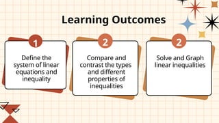
2. Define the
system of linear
equations and
inequality
1 2
Compare and
contrast the types
and different
properties of
inequalities
Learning Outcomes
2
Solve and Graph
linear inequalities

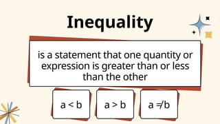
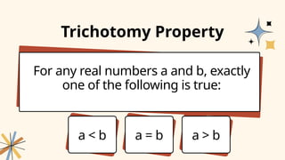
3. is a statement that one quantity or
expression is greater than or less
than the other
Inequality
a < b a > b a ≠ b

4. Try to read:
1
a > b
2
a < b
3
a b
≥
a is greater than b
a is less than b
a is greater than or
equal b
4
a b
≤
a is less than or equal
b
5
a < b < c
b is greater than a
but less than c

5. Properties of
Inequalities

6. For any real numbers a and b, exactly
one of the following is true:
Trichotomy Property
a < b a = b a > b

7. For any real numbers a, b, and c:
a. If a < b, then a ± c < b ± c
b. If a > b, then a ± c > b ± c
Addition Property

8. For any real numbers a, b, and c:
a. If a < b and c is positive, then ac <
bc
b. If a > b and c is positive, then ac >
Multiplication Property

9. For all real numbers a, b, and c:
a. If a < b and c is positive, then <
b. If a < b and c is negative, then >
Division Property

10. Types of
Inequalities

11. Absolute Inequality
1
It is a condition where the
inequality is true for all values of
the unknown involved.
x2
+ 7 > 0

12. Conditional Inequality
It is a condition where the
inequality is true for certain values
of the unknown involved.
4x – 3 > 0
2

13. Practice Questions
1
2
3x – 1 > 4
x4
- 6 > 4
3 X3
> 8
2x + 3 > 8

14. Graphs of
Inequalities

15. Steps in graphing
1 Replace the inequality with an
equal sign and then plot the graph
of the equation

16. Steps in graphing
2 Select a test point lying in one of
the half-planes determined by the
graph and substitute the values of
x and y into the given inequality.

17. Steps in graphing
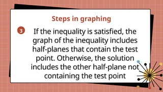
3 If the inequality is satisfied, the
graph of the inequality includes
half-planes that contain the test
point. Otherwise, the solution
includes the other half-plane not
containing the test point

18. Example:
x > 5
-7 - 6 -5 - 4 - 3 - 2 -1 0 1 2 3 4 5 6 7 8 9

19. Example:
2x + y 8
≤
2x + y = 16
Let x = 0
2x + y = 8
2 (0) + y =
8
y = 8
Let y = 0
2x + y = 8
2x + 0 =
8
2x = 8
x = 4
(0, 8) (4, 0)

20. Example:
x + 2y 4
≥
Find the solution set of the given
inequalities in a graphical method x + 2y ≥
4 and 2x + y 6
≤
2x + y 4
≤

21. Example:
Find the solution set of
the given inequalities
in a graphical method
x + 2y 4 and
≥
2x + y 6
≤

22. Any Questions?

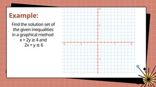
23. 1. Sketch the graph of
the following
inequalities
a. x + 3y 9
≤
b. 4x – y 8
≥
c. x + 3y > 12
Try to answer these:
1. Sketch the graph of the
following inequalities by x and
y-intercept
a. 3x + 5y 15
≤ ; 5x – 3y
15
≤
b. x + y 6
≤ ; 2x – y 6
≥

25. Have you ever been
in a situation where
you have to choose
between two
things?

26. Geometry of
Linear
Programming

28. Programming
Producing a plan or procedure that
determines the solution to a
problem.

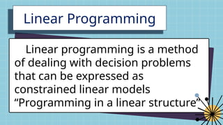
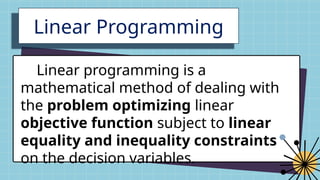
29. Linear Programming
Linear programming is a method
of dealing with decision problems
that can be expressed as
constrained linear models
“Programming in a linear structure”

30. Linear Programming
Linear programming is a
mathematical method of dealing with
the problem optimizing linear
objective function subject to linear
equality and inequality constraints
on the decision variables.

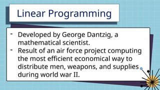
31. Linear Programming
- Developed by George Dantzig, a
mathematical scientist.
- Result of an air force project computing
the most efficient economical way to
distribute men, weapons, and supplies
during world war II.

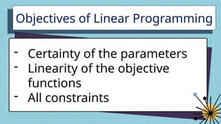
32. Objectives of Linear Programming
- Certainty of the parameters
- Linearity of the objective
functions
- All constraints

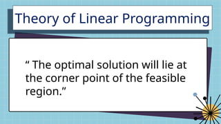
33. Theory of Linear Programming
“ The optimal solution will lie at
the corner point of the feasible
region.”

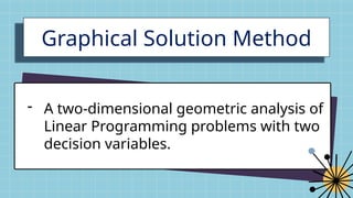
34. Graphical Solution Method
- A two-dimensional geometric analysis of
Linear Programming problems with two
decision variables.

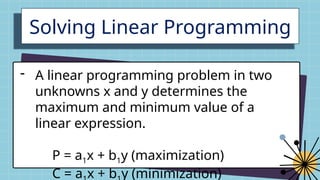
35. Solving Linear Programming
- A linear programming problem in two
unknowns x and y determines the
maximum and minimum value of a
linear expression.
P = a1x + b1y (maximization)
C = a x + b y (minimization)

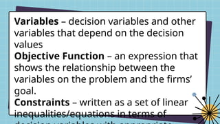
36. Variables – decision variables and other
variables that depend on the decision
values
Objective Function – an expression that
shows the relationship between the
variables on the problem and the firms’
goal.
Constraints – written as a set of linear
inequalities/equations in terms of

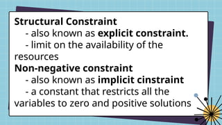
37. Structural Constraint
- also known as explicit constraint.
- limit on the availability of the
resources
Non-negative constraint
- also known as implicit cinstraint
- a constant that restricts all the
variables to zero and positive solutions

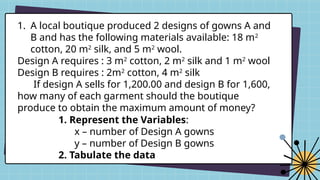
38. 1. A local boutique produced 2 designs of gowns A and
B and has the following materials available: 18 m2
cotton, 20 m2
silk, and 5 m2
wool.
Design A requires : 3 m2
cotton, 2 m2
silk and 1 m2
wool
Design B requires : 2m2
cotton, 4 m2
silk
If design A sells for 1,200.00 and design B for 1,600,
how many of each garment should the boutique
produce to obtain the maximum amount of money?
1. Represent the Variables:
x – number of Design A gowns
y – number of Design B gowns
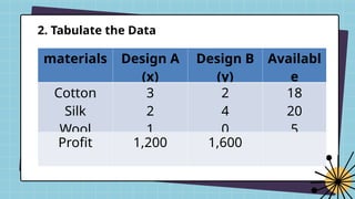
2. Tabulate the data

39. 2. Tabulate the Data
materials Design A
(x)
Design B
(y)
Availabl
e
Cotton
Silk
Wool
3
2
1
2
4
0
18
20
5
Profit 1,200 1,600

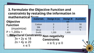
40. 3. Formulate the Objective Function and
constraints by restating the information in
mathematical form.
materials Design A (x) Design B
(y)
Available
Cotton
Silk
Wool
3
2
1
2
4
0
18
20
5
Profit 1,200 1,600
Objective
Function
(maximize)
P = 1,200x +
1,600y
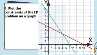
Structural Constraints
3x + 2y 18
≤
2x + 4y 20
≤
x 5
≤
Non negativity
Constraints
x 0, y 0
≥ ≥

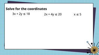
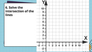
41. Solve for the coordinates
3x + 2y 18
≤ 2x + 4y 20
≤ x 5
≤

42. 4. Plot the
constraints of the LP
problem on a graph

43. 5. Identify the
feasible region
Feasible
region

44. 6. Solve the
intersection of the
lines

45. 7. Substitute the coordinates at the extreme
points
Extreme Points Values of the objective function
(0, 5)
(5, 0)
(4, 3)
(5, 1.5)
P = 1,200x + 1,600y
8. Formulate the decision