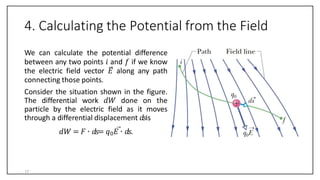
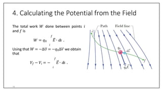
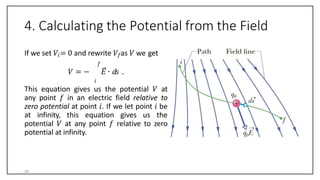
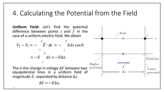
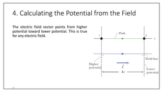
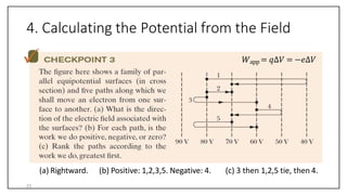
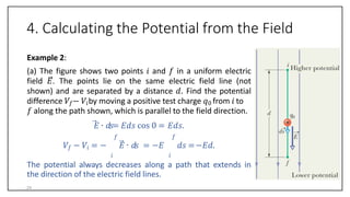
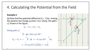
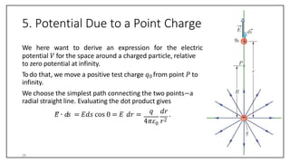
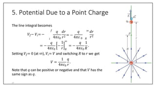
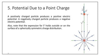
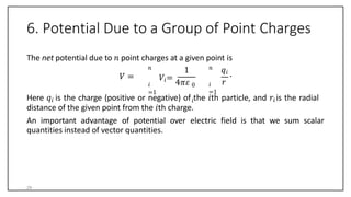
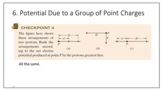
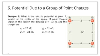
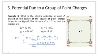
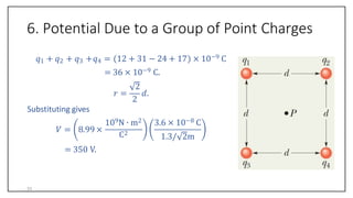
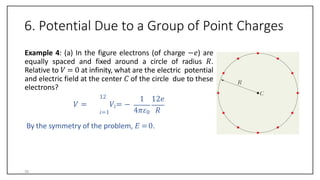
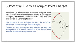
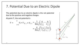
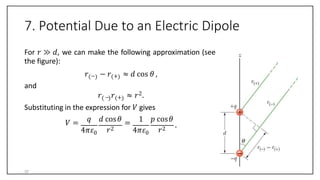
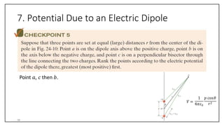
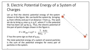
Chapter 24
Electric Potential
1
1. Electric Potential Energy
When an electrostatic force acts between two or more charged particles within a
system of particle, we can assign an electric potential energy 𝑈 to the system. If the
system changes its configuration from state 𝑖 to state 𝑓, the electrostatic force does
work 𝑊 on the particles. The resulting change ∆𝑈 in potential energy of the system
is
∆𝑈 = 𝑈𝑓 − 𝑈𝑖 = −𝑊.
The work done by the electrostatic force is path independent, since the
electrostatic force is conservative.
We take the reference configuration of a system of charged particles to be that in
which the particles are all infinitely separated from each other. The energy of this
reference configuration is set to be zero.
2
1. Electric Potential Energy
Suppose that several charged particles come together from initially infinite
separations (state 𝑖) to form a system of neighboring particles (state 𝑓). Let the
initial potential energy 𝑈𝑖 be zero and let 𝑊∞ represents the work done by the
electrostatic force between the particles during the process. The final potential
energy 𝑈 of the system is
𝑈 =−𝑊∞.
3
1. Electric Potential Energy
(a) Negative work.
(b) Increases.
𝑊 =−∆𝑈
4
1. Electric Potential Energy
Example 1: Electrons are continually being knocked out
of air molecules in the atmosphere by cosmic-ray
particles coming in from space. Once released, each
electron experiences an electrostatic force 𝐹 due to
the electric field 𝐸 that is produced in the atmosphere
by charged particles already on Earth. Near Earth’s
surface the electric field has the magnitude 𝐸 = 150 N
/C and is directed downward. What is the change ∆𝑈
in the electric potential energy of a released electron
when the electrostatic force causes it to move vertically
upward through a distance 𝑑 = 520m?
5
1. Electric Potential Energy
The work 𝑊 done on the electron by the electrostatic
force is
𝑊 = 𝐹 ∙ 𝑑 = 𝐹𝑑 cos 0 = 𝐸𝑒𝑑
= 150 N/C 1.60 × 10⁻¹⁹ C 520 m
= 1.2 × 10⁻¹⁴ J.
∆𝑈 = −𝑊 = −1.2 × 10⁻¹⁴ J.
6
2. Electric Potential
The potential energy of a charged particle in an electric field depends on the charge
magnitude. The potential energy per unit charge, however, has a unique value at
any point in an electric field.
For example, a proton that has potential energy of 2.40 × 10⁻¹⁷ J in an electric
field has potential per unit charge of
2.40 × 10⁻¹⁷ J
1.60 × 10⁻¹⁹ C
= 150 J/C.
Suppose we next replace the proton with an alpha particle (charge +2𝑒). The alpha
particle would have electric potential energy of 4.80 × 10⁻¹⁷ J. However, the
potential energy per unit charge would be the same 150 J/C.
7
2. Electric Potential
The potential energy per unit charge 𝑈/𝑞 is a characteristic only of the electric
field. The potential energy per unit charge at a point in an electric field is called the
electric potential 𝑉 (or simply potential) at that point. Thus,
𝑈
𝑞
𝑉 = .
Note that 𝑉 is a scalar, not a vector.
The electric potential difference ∆𝑉 between any two points 𝑖 and 𝑓 in an electric
field is equal to the difference in potential energy per unit charge between the two
points:
𝑈𝑓 𝑈𝑖 ∆𝑈
∆𝑉 = 𝑉𝑓 −𝑉𝑖 =
𝑞
−
𝑞
=
𝑞
.
8
2. Electric Potential
Substituting −𝑊 for ∆𝑈 we find that
𝑊
∆𝑉 = 𝑉𝑓 − 𝑉𝑖 = −
𝑞
.
The potential difference between two points is the negative of the work done by
the electrostatic force on a unit charge as it moved from one point to the other.
If we set 𝑈𝑖 = 0 at infinity as our reference potential energy, 𝑉 must be zero there
too. The electric potential at any point in an electric field is thus
𝑞 𝑞
𝑈 𝑊∞
𝑉 = = − .
The SI unit for potential 𝑉 is joule per coulomb or volt (V):
1 volt = 1 joul per coulomb.
9
2. Electric Potential
In terms of this unit, we can write the electric field in a more convenient unit:
1
N
C
= 1
N 1 V 1 J V
C 1 J/C 1 N ∙ m m
= 1 .
We can also define an energy unit that is convenient for energy scale of the atomic
physics; the electron-volt (eV). One electron-volt is the energy equal to the work
required to move a single elementary charge 𝑒 through a potential difference of
one volt (𝑞∆𝑉). Thus
1 eV = 𝑒 1 V = 1.60 × 10⁻¹⁹ C 1 J/C = 1.60 × 10⁻¹⁹ J.
10
2. Electric Potential
Work Done by an Applied Force
Suppose we move a particle of charge 𝑞 from point 𝑖 to point 𝑓 in an electric field
by applying a force to it. By the work-kinetic energy theorem,
∆𝐾 = 𝑊app +𝑊,
where 𝑊app is the work done by the applied force and 𝑊 is the work done by the
electric field.
If ∆𝐾 = 0, we obtainthat
𝑊app = −𝑊.
Using that ∆𝑈 = −𝑊, we obtainthat
𝑊app = ∆𝑈 = 𝑞∆𝑉.
11
2. Electric Potential
(a) Positive work.
(b) Higher potential.
𝑊app = ∆𝑈 = 𝑞∆𝑉
12
3. Equipotential Surfaces
An equipotential surface is composed of adjacent points that have the same
electric potential. No net work 𝑊 is done on a charged particle by an electric field
when the particle’s initial point 𝑖 and final point 𝑓 lie on the same equipotential
surface.
13
3. Equipotential Surfaces
𝑉1= 100 V
𝑉2 = 80 V
𝑉3 = 60 V
𝑉4 = 40 V
14
3. Equipotential Surfaces
15
3. Equipotential Surfaces
Equipotential surfaces are perpendicular to the electric field 𝐸.
If 𝐸 were not perpendicular to an equipotential surface, it would have a component
along the surface. This component would then do work on a charged particle as it
moved along the surface.
16
4. Calculating the Potential from the Field
We can calculate the potential difference
between any two points 𝑖 and 𝑓 if we know
the electric field vector 𝐸 along any path
connecting those points.
Consider the situation shown in the figure.
The differential work 𝑑𝑊 done on the
particle by the electric field as it moves
through a differential displacement 𝑑𝑠is
𝑑𝑊 = 𝐹 ∙ 𝑑𝑠= 𝑞0𝐸 ∙ 𝑑𝑠.
17
4. Calculating the Potential from the Field
The total work 𝑊 done between points 𝑖
and 𝑓 is
𝑓
𝑊 = 𝑞0 𝐸 ∙ 𝑑𝑠 .
𝑖
Using that 𝑊 = −∆𝑈 = −𝑞0∆𝑉 we obtain
that
𝑓
𝑉𝑓 − 𝑉𝑖 = − 𝐸 ∙ 𝑑𝑠 .
𝑖
18
4. Calculating the Potential from the Field
If we set 𝑉𝑖= 0 and rewrite 𝑉𝑓as 𝑉 we get
𝑓
𝑉 = − 𝐸 ∙ 𝑑𝑠 .
𝑖
This equation gives us the potential 𝑉 at
any point 𝑓 in an electric field relative to
zero potential at point 𝑖. If we let point 𝑖 be
at infinity, this equation gives us the
potential 𝑉 at any point 𝑓 relative to zero
potential at infinity.
19
4. Calculating the Potential from the Field
If we set 𝑉𝑖= 0 and rewrite 𝑉𝑓as 𝑉 we get
𝑓
𝑉 = − 𝐸 ∙ 𝑑𝑠 .
𝑖
This equation gives us the potential 𝑉 at
any point 𝑓 in an electric field relative to
zero potential at point 𝑖. If we let point 𝑖 be
at infinity, this equation gives us the
potential 𝑉 at any point 𝑓 relative to zero
potential at infinity.
20
4. Calculating the Potential from the Field
Uniform Field: Let’s find the potential
difference between points 𝑖 and 𝑓 in the
case of a uniform electric field. We obtain
𝑓 𝑓
𝑉𝑓 − 𝑉𝑖 = − 𝐸 ∙ 𝑑𝑠 = − 𝐸𝑑𝑠 cos0
𝑖 𝑖
𝑓
= −𝐸 𝑑𝑠 =−𝐸∆𝑥.
𝑖
The is the change in voltage ∆𝑉 between two
equipotential lines in a uniform field of
magnitude 𝐸, separated by distance ∆𝑥
∆𝑉 =−𝐸∆𝑥.
21
4. Calculating the Potential from the Field
The electric field vector points from higher
potential toward lower potential. This is true
for any electric field.
22
4. Calculating the Potential from the Field
(a) Rightward. (b) Positive: 1,2,3,5. Negative: 4. (c) 3 then 1,2,5 tie, then 4.
𝑊app = 𝑞∆𝑉 = −𝑒∆𝑉
23
4. Calculating the Potential from the Field
Example 2:
(a) The figure shows two points 𝑖 and 𝑓 in a uniform electric
field 𝐸. The points lie on the same electric field line (not
shown) and are separated by a distance 𝑑. Find the potential
difference 𝑉𝑓− 𝑉𝑖by moving a positive test charge 𝑞0 from 𝑖 to
𝑓 along the path shown, which is parallel to the field direction.
𝐸 ∙ 𝑑𝑠= 𝐸𝑑𝑠 cos 0 = 𝐸𝑑𝑠.
𝑓 𝑓
𝑉𝑓 − 𝑉𝑖 = − 𝐸 ∙ 𝑑𝑠 = −𝐸 𝑑𝑠 =−𝐸𝑑.
𝑖 𝑖
The potential always decreases along a path that extends in
the direction of the electric field lines.
24
4. Calculating the Potential from the Field
Example 2:
(b) Now find the potential difference 𝑉𝑓− 𝑉𝑖by moving
the positive test charge 𝑞0 from 𝑖 to 𝑓 along the path 𝑖
𝑐𝑓 shown in the figure.
𝑉𝑓 − 𝑉𝑖 = 𝑉𝑓 −𝑉𝑐.
Along path 𝑐𝑓
𝐸 ∙ 𝑑𝑠= 𝐸𝑑𝑠 cos 45°.
𝑓 𝑓
𝑉𝑓 − 𝑉𝑖 = − 𝐸 ∙ 𝑑𝑠 = −𝐸 cos 45° 𝑑𝑠
𝑐
= −𝐸 cos 45° 2𝑑
𝑐
= −𝐸𝑑.
25
5. Potential Due to a Point Charge
We here want to derive an expression for the electric
0
potential 𝑉 for the space around a charged particle, relative
to zero potential at infinity.
Todo that, we move a positive test charge 𝑞0 from point 𝑃 to
infinity.
We choose the simplest path connecting the two points−a
radial straight line. Evaluating the dot product gives
𝑞 𝑑𝑟
𝐸 ∙ 𝑑𝑠 = 𝐸𝑑𝑠 cos 0 = 𝐸 𝑑𝑟 = .
4𝜋𝜀 𝑟2
26
5. Potential Due to a Point Charge
4𝜋𝜀0
𝑞 𝑑𝑟 𝑞
𝑟2 = −
4𝜋𝜀 0
∞ 𝑑𝑟
𝑟2
The line integral becomes
𝑓
𝑉𝑓− 𝑉𝑖= −
𝑖
𝑞
4𝜋𝜀0 𝑟 𝑅
1 ∞
= − − = −
𝑅
𝑞 1
4𝜋𝜀0 𝑅
.
Setting 𝑉𝑓= 0 (at ∞), 𝑉𝑖= 𝑉 and switching 𝑅 to 𝑟 we get
𝑉 =
1 𝑞
4𝜋𝜀0 𝑟
.
Note that 𝑞 can be positive or negative and that 𝑉 has the
same sign as 𝑞.
27
5. Potential Due to a Point Charge
A positively charged particle produces a positive electric
potential. A negatively charged particle produces a negative
electric potential.
Also, note that the expression for 𝑉 holds outside or on the
surface of a spherically symmetric charge distribution.
28
6. Potential Due to a Group of Point Charges
The net potential due to 𝑛 point charges at a given point is
𝑖
=1
𝑛
𝑉 =
1
𝑉𝑖=
4𝜋𝜀
𝑛
𝑖
=1
𝑞𝑖
0
𝑖
.
𝑟
Here 𝑞𝑖 is the charge (positive or negative) of the 𝑖th particle, and 𝑟𝑖is the radial
distance of the given point from the 𝑖th charge.
An important advantage of potential over electric field is that we sum scalar
quantities instead of vector quantities.
29
6. Potential Due to a Group of Point Charges
All the same.
30
6. Potential Due to a Group of Point Charges
Example 3: What is the electric potential at point P,
located at the center of the square of point charges
shown in the figure? The distance 𝑑 = 1.3 m, and the
charges are
𝑞1 = 12 nC,
𝑞3 = −24 nC,
𝑞2 = 31 nC,
𝑞4 = 17 nC.
31
6. Potential Due to a Group of Point Charges
Example 3: What is the electric potential at point P,
located at the center of the square of point charges
shown in the figure? The distance 𝑑 = 1.3 m, and the
charges are
𝑞1 = 12 nC,
𝑞3 = −24 nC,
𝑞2 = 31 nC,
𝑞4 = 17 nC.
𝑖
=1
𝑖
4
𝑉 = 𝑉 =
4𝜋𝜀0
1 𝑞1
+
𝑞2
+
𝑞3
+
𝑞4
𝑟 𝑟 𝑟 𝑟
=
1 𝑞1 + 𝑞2 + 𝑞3 + 𝑞4
4𝜋𝜀0 𝑟
32
6. Potential Due to a Group of Point Charges
𝑞1 + 𝑞2 + 𝑞3 +𝑞4 = 12 + 31 − 24 + 17 × 10−9 C
= 36 × 10−9 C.
2
2
𝑟 = 𝑑.
109N ∙ m2
C2
3.6 × 10⁻⁸ C
1.3/ 2m
Substituting gives
𝑉 = 8.99 ×
= 350 V.
33
6. Potential Due to a Group of Point Charges
Example 4: (a) In the figure electrons (of charge −𝑒) are
equally spaced and fixed around a circle of radius 𝑅.
Relative to 𝑉 = 0 at infinity, what are the electric potential
and electric field at the center 𝐶 of the circle due to these
electrons?
12
𝑉 = 𝑉𝑖= −
𝑖=1
1 12𝑒
4𝜋𝜀0 𝑅
By the symmetry of the problem, 𝐸 =0.
34
6. Potential Due to a Group of Point Charges
Example 4: (b) If the electrons are moved along the circle
until they are nonuniformly spaced over a 120° arc (see
the figure), what then is the potential at 𝐶? How does the
electric field at 𝐶 change (if at all)?
The potential is not changed because the distances
between 𝐶 and each charge are not changed.
The electric field is no longer zero, however, because the
arrangement is no longer symmetric. A net field is now
directed toward the charge distribution.
35
7. Potential Due to an Electric Dipole
The potential due to an electric dipole is the net potential
due to the positive and negative charges.
At point 𝑃, the net potential is
2
𝑉 = 𝑉𝑖= 𝑉 +
𝑖=1
+ 𝑉−
0
1 𝑞 𝑞
= −
4𝜋𝜀 𝑟 𝑟
+ −
=
4𝜋𝜀0
𝑞 𝑟 − − 𝑟 +
𝑟 + 𝑟 −
.
36
7. Potential Due to an Electric Dipole
For 𝑟 ≫ 𝑑, we can make the following approximation (see
the figure):
𝑟 − − 𝑟 + ≈ 𝑑 cos 𝜃 ,
and
𝑟 − 𝑟 + ≈ 𝑟2.
Substituting in the expression for 𝑉 gives
𝑉 =
4𝜋𝜀0
𝑞 𝑑 cos𝜃
𝑟2
=
4𝜋𝜀0
1 𝑝 cos𝜃
𝑟2
.
37
7. Potential Due to an Electric Dipole
Point 𝑎, 𝑐 then 𝑏.
𝑉 =
4𝜋𝜀0
1 𝑝 cos𝜃
38
𝑟2
7. Potential Due to an Electric Dipole
Induced Dipole Moment
39
7. Potential Due to an Electric Dipole
Induced Dipole Moment
40
8. Calculating the Field from the Potential
Let us see graphically how we can calculate the field from the potential. If we know
the potential 𝑉 at all points near a charge distribution, we can draw a family of
equipotential surfaces. The electric field lines, sketched perpendicular to those
surfaces, reveal the variation of 𝐸.
We want now to write the mathematical equivalence of this graphical procedure.
41
8. Calculating the Field from the Potential
The figure shows cross sections of a family of closely
spaced equipotential surfaces.
The potential difference between each pair of
adjacent surfaces is 𝑑𝑉. The electric field 𝐸 at any
point 𝑃 is perpendicular to the equipotential surface
through 𝑃.
Suppose that a positive test charge 𝑞0 moves
through a displacement 𝑑𝑠 from an equipotential
surface to the adjacent surface.
The work 𝑑𝑊 done by the electric field on the test
charge is
𝑑𝑊 =−𝑞0𝑑𝑉.
42
8. Calculating the Field from the Potential
The work 𝑑𝑊 can also be written as
𝑑𝑊 = 𝐹 ∙ 𝑑𝑠= 𝑞0𝐸 ∙ 𝑑𝑠= 𝑞0𝐸𝑑𝑠 cos 𝜃.
Equating the two expression for 𝑑𝑊 yields
−𝑞0𝑑𝑉 = 𝑞0𝐸𝑑𝑠 cos 𝜃 ,
or
𝐸 cos 𝜃 = −
𝑑𝑉
𝑑𝑠
.
𝐸 cos 𝜃 is the component of 𝐸 in the direction of
𝑑𝑠. Thus,
𝜕𝑉
𝐸𝑠 = −
𝜕𝑠
.
43
8. Calculating the Field from the Potential
The component of 𝐸 in any direction is the negative
of the rate at which the electric potential changes
with distance in that direction.
If we take 𝑑𝑠 to be along the 𝑥, 𝑦 and 𝑧 axes, we
obtain the 𝑥, 𝑦 and 𝑧 components of 𝐸 at any point:
𝜕𝑉
𝐸𝑥 = −
𝜕𝑥
;
𝜕𝑉
𝐸𝑦 = −
𝜕𝑦
;
𝜕𝑉
𝐸z = −
𝜕𝑧
.
If we know the function 𝑉 𝑥, 𝑦, 𝑧 , we can find the
components of 𝐸 at any point.
44
8. Calculating the Field from the Potential
When the electric field 𝐸 is uniform, we write that
∆𝑉
∆𝑠
𝐸 = − .
where 𝑠 is perpendicular to the equipotential surfaces. The component of the
electric field is zero in any direction parallel to the equipotential surfaces because
there is no change in potential along an equipotential surface.
45
8. Calculating the Field from the Potential
𝐸 =−
∆𝑉
∆𝑠
(a) 2, then 3 & 1.
(b) 3.
(c) Accelerates
leftward.
46
8. Calculating the Field from the Potential
Example 5: Starting with the expression for the potential due to an electric dipole,
𝑉 =
4𝜋𝜀0
1 𝑝 cos𝜃
𝑟2
.
derive an expression for the radial component of electric field due to the electric
dipole.
𝐸𝑟 = −
𝜕𝑟
= −
4𝜋𝜀0
𝜕𝑉 𝑝 cos 𝜃 𝑑 1
= −
4𝜋𝜀0
𝑝 cos 𝜃 2
𝑟3
− =
2𝜋𝜀0
𝑑𝑟 𝑟2
1 𝑝 cos𝜃
𝑟3
.
47
8. Calculating the Field from the Potential
Example 6: The electric potential at any point on the central axis of a uniformly
charged disk is given by
𝑉 =
𝜎
2𝜀0
𝑧2 + 𝑅2 − 𝑧 .
Starting with this expression, derive an expression for the electric field at any point
on the axis of the disk.
𝑧
𝜕𝑧 2𝜀0 𝑑𝑧
𝜕𝑉 𝜎 𝑑
𝐸 = − = 𝑧 − 𝑧2 +𝑅2
=
2𝜀0
𝜎 𝑧
𝑧2 + 𝑅2
1 − .
48
9. Electric Potential Energy of a System of
Charges
The electric potential energy of a system of fixed point charges is equal to the work
that must be done by an external agent to assemble the system, bringing each
charge in from an infinite distance.
We assume that the charges are stationary at both the initial and final states.
50
9. Electric Potential Energy of a System of
Charges
Let us find the electric potential energy of the system
shown in the figure. We can build the system by bringing
𝑞2 from infinity and put it at distance 𝑟 from 𝑞1. The work
we do to bring 𝑞2 near 𝑞1 is 𝑞2𝑉, where 𝑉 is the potential
that has been set up by 𝑞1. Thus, the electric potential of
the pair of point charges shown in the figure is
𝑈 = 𝑊app = 𝑞2𝑉 =
4𝜋𝜀0 𝑟
1 𝑞1𝑞2
.
𝑈 has the same sign as that of 𝑞1𝑞2.
The total potential energy of a system of several particles
is the sum of the potential energies for every pair of
particles in the system.
51
9. Electric Potential Energy of a System of
Charges
Example 7: The figure shows three point charges held in
fixed positions by forces that are not shown. What is the
electric potential energy 𝑈 of this system of charges?
Assume that 𝑑 = 12 cm andthat
𝑞1 = +𝑞, 𝑞2 = −4𝑞, 𝑞3 = +2𝑞,
and 𝑞 = 150nC.
The electric potential energy of the system (energy required
to assemble the system) is
𝑈 = 𝑈12 + 𝑈13 +𝑈23
=
1 𝑞1𝑞2
+
1 𝑞1𝑞3
+
1 𝑞2𝑞3
.
4𝜋𝜀0 𝑑 4𝜋𝜀0 𝑑 4𝜋𝜀0 𝑑
52
9. Electric Potential Energy of a System of
Charges
𝑈 =
4𝜋𝜀0
+ +
1 𝑞 −4𝑞 1 𝑞 2𝑞 1 −4𝑞 2𝑞
4𝜋𝜀0 𝑑 𝑑 4𝜋𝜀0 𝑑
= −
4𝜋𝜀0𝑑
= 8.99 × 10¹²
10𝑞2 N ∙ m2
C2
10 150 × 10−9C
0.12 m
= −17 mJ.
53
9. Electric Potential Energy of a System of
Charges
Example 8: An alpha particle (two protons, two neutrons)
moves into a stationary gold atom (79 protons, 118
neutrons), passing through the electron region that
surrounds the gold nucleus like a shell and headed
directly toward the nucleus. The alpha particle slows until
it momentarily stops when its center is at radial distance 𝑟
= 9.23 fm from the nuclear center. Then it moves back
along its incoming path. (Because the gold nucleus is
much more massive than the alpha particle, we can
assume the gold nucleus does not move.) What was the
kinetic energy 𝐾𝑖of the alpha particle when it was initially
far away (hence external to the gold atom)? Assume that
the only force acting between the alpha particle and the
gold nucleus is the (electrostatic) Coulomb force.
54
9. Electric Potential Energy of a System of
Charges
During the entire process, the mechanical energy of the
alpha particle-gold atom system is conserved.
𝐾𝑖 + 𝑈𝑖 = 𝐾𝑓 + 𝑈𝑓.
𝑈𝑖 is zero because the atom is neutral. 𝑈𝑓 is the electric
potential energy of the alpha particle-nucleus system. The
electron shell produces zero electric field inside it. 𝐾𝑓 is
zero.
𝐾𝑖 = 𝑈𝑓 =
1 2𝑒 79𝑒
4𝜋𝜀0 9.23 × 10⁻¹⁵ m
= 3.94 × 10⁻⁹ J
= 24.6 MeV.
55
10. Potential of a Charged Isolated Conductor
In Ch. 23, we concluded that 𝐸 = 0 within an isolated conductor. We then used
Gauss’ law to prove that all excess charge placed on a conductor lies entirely on its
surface. Here we use the first of these facts to prove an extension of the second:
‘An excess charge placed on an isolated conductor will distribute itself on the
surface of that conductor so that all points of the conductor—whether on the
surface or inside—come to the same potential. This is true even if the conductor
has an internal cavity and even if that cavity contains a net charge.’
Toprove this fact we use that
𝑓
𝑉𝑓 − 𝑉𝑖 = − 𝐸 ∙ 𝑑𝑠 .
𝑖
Since 𝐸 = 0 for all point within a conductor, 𝑉𝑓= 𝑉𝑖for all possible pairs of points 𝑖
and 𝑓 in the conductor.
56
10. Potential of a Charged Isolated Conductor
The figure shows the potential against radial
distance 𝑟 from the center from an isolated
spherical conducting shell of radius 𝑅 = 1.0 m and
charge 𝑞 = 0.10𝜇C.
For points outside the shell up to its surface, 𝑉 𝑟
= 𝑘 𝑞/𝑟. Now assume that we push a test charge
though a hole in the shell. No extra work is required
to do this because 𝐸 becomes zero once the test
charge gets inside the shell. Thus, the potential at
all points inside the shell has the same value as that
of its surface.
57
10. Potential of a Charged Isolated Conductor
The figure shows the variation of the electric field
with radial distance for the same shell. Everywhere
inside the shell 𝐸 = 0. Outside the shell 𝐸 = 𝑘 𝑞
/𝑟2. The electric field can be obtained from the
potential using 𝐸 =−𝑑𝑉/𝑑𝑟.
58
10. Potential of a Charged Isolated Conductor
Spark Discharge from a Charged Conductor
On nonspherical conductors, a surface charge does
not distribute itself uniformly over the surface of
the conductor. At sharp points or sharp edges, the
surface charge density—and thus the external
electric field, which is proportional to it—may reach
very high values. The air around such sharp points
or edges may become ionized, producing the
corona discharge.
59
10. Potential of a Charged Isolated Conductor
Isolated Conductor in an External Electric Field
If an isolated conductor is placed in an external
electric field, all points of the conductor still come
to a single potential regardless of whether the
conductor has an excess charge or not. The free
conduction electrons distribute themselves on the
surface in such a way that the electric field they
produce at interior points cancels the external
electric field. Furthermore, the electron distribution
causes the net electric field at all points on the
surface to be perpendicular to the surface.
64

Chapter 24 till slide 40.pptx

  • 1.
  • 2.
    1. Electric PotentialEnergy When an electrostatic force acts between two or more charged particles within a system of particle, we can assign an electric potential energy 𝑈 to the system. If the system changes its configuration from state 𝑖 to state 𝑓, the electrostatic force does work 𝑊 on the particles. The resulting change ∆𝑈 in potential energy of the system is ∆𝑈 = 𝑈𝑓 − 𝑈𝑖 = −𝑊. The work done by the electrostatic force is path independent, since the electrostatic force is conservative. We take the reference configuration of a system of charged particles to be that in which the particles are all infinitely separated from each other. The energy of this reference configuration is set to be zero. 2
  • 3.
    1. Electric PotentialEnergy Suppose that several charged particles come together from initially infinite separations (state 𝑖) to form a system of neighboring particles (state 𝑓). Let the initial potential energy 𝑈𝑖 be zero and let 𝑊∞ represents the work done by the electrostatic force between the particles during the process. The final potential energy 𝑈 of the system is 𝑈 =−𝑊∞. 3
  • 4.
    1. Electric PotentialEnergy (a) Negative work. (b) Increases. 𝑊 =−∆𝑈 4
  • 5.
    1. Electric PotentialEnergy Example 1: Electrons are continually being knocked out of air molecules in the atmosphere by cosmic-ray particles coming in from space. Once released, each electron experiences an electrostatic force 𝐹 due to the electric field 𝐸 that is produced in the atmosphere by charged particles already on Earth. Near Earth’s surface the electric field has the magnitude 𝐸 = 150 N /C and is directed downward. What is the change ∆𝑈 in the electric potential energy of a released electron when the electrostatic force causes it to move vertically upward through a distance 𝑑 = 520m? 5
  • 6.
    1. Electric PotentialEnergy The work 𝑊 done on the electron by the electrostatic force is 𝑊 = 𝐹 ∙ 𝑑 = 𝐹𝑑 cos 0 = 𝐸𝑒𝑑 = 150 N/C 1.60 × 10⁻¹⁹ C 520 m = 1.2 × 10⁻¹⁴ J. ∆𝑈 = −𝑊 = −1.2 × 10⁻¹⁴ J. 6
  • 7.
    2. Electric Potential Thepotential energy of a charged particle in an electric field depends on the charge magnitude. The potential energy per unit charge, however, has a unique value at any point in an electric field. For example, a proton that has potential energy of 2.40 × 10⁻¹⁷ J in an electric field has potential per unit charge of 2.40 × 10⁻¹⁷ J 1.60 × 10⁻¹⁹ C = 150 J/C. Suppose we next replace the proton with an alpha particle (charge +2𝑒). The alpha particle would have electric potential energy of 4.80 × 10⁻¹⁷ J. However, the potential energy per unit charge would be the same 150 J/C. 7
  • 8.
    2. Electric Potential Thepotential energy per unit charge 𝑈/𝑞 is a characteristic only of the electric field. The potential energy per unit charge at a point in an electric field is called the electric potential 𝑉 (or simply potential) at that point. Thus, 𝑈 𝑞 𝑉 = . Note that 𝑉 is a scalar, not a vector. The electric potential difference ∆𝑉 between any two points 𝑖 and 𝑓 in an electric field is equal to the difference in potential energy per unit charge between the two points: 𝑈𝑓 𝑈𝑖 ∆𝑈 ∆𝑉 = 𝑉𝑓 −𝑉𝑖 = 𝑞 − 𝑞 = 𝑞 . 8
  • 9.
    2. Electric Potential Substituting−𝑊 for ∆𝑈 we find that 𝑊 ∆𝑉 = 𝑉𝑓 − 𝑉𝑖 = − 𝑞 . The potential difference between two points is the negative of the work done by the electrostatic force on a unit charge as it moved from one point to the other. If we set 𝑈𝑖 = 0 at infinity as our reference potential energy, 𝑉 must be zero there too. The electric potential at any point in an electric field is thus 𝑞 𝑞 𝑈 𝑊∞ 𝑉 = = − . The SI unit for potential 𝑉 is joule per coulomb or volt (V): 1 volt = 1 joul per coulomb. 9
  • 10.
    2. Electric Potential Interms of this unit, we can write the electric field in a more convenient unit: 1 N C = 1 N 1 V 1 J V C 1 J/C 1 N ∙ m m = 1 . We can also define an energy unit that is convenient for energy scale of the atomic physics; the electron-volt (eV). One electron-volt is the energy equal to the work required to move a single elementary charge 𝑒 through a potential difference of one volt (𝑞∆𝑉). Thus 1 eV = 𝑒 1 V = 1.60 × 10⁻¹⁹ C 1 J/C = 1.60 × 10⁻¹⁹ J. 10
  • 11.
    2. Electric Potential WorkDone by an Applied Force Suppose we move a particle of charge 𝑞 from point 𝑖 to point 𝑓 in an electric field by applying a force to it. By the work-kinetic energy theorem, ∆𝐾 = 𝑊app +𝑊, where 𝑊app is the work done by the applied force and 𝑊 is the work done by the electric field. If ∆𝐾 = 0, we obtainthat 𝑊app = −𝑊. Using that ∆𝑈 = −𝑊, we obtainthat 𝑊app = ∆𝑈 = 𝑞∆𝑉. 11
  • 12.
    2. Electric Potential (a)Positive work. (b) Higher potential. 𝑊app = ∆𝑈 = 𝑞∆𝑉 12
  • 13.
    3. Equipotential Surfaces Anequipotential surface is composed of adjacent points that have the same electric potential. No net work 𝑊 is done on a charged particle by an electric field when the particle’s initial point 𝑖 and final point 𝑓 lie on the same equipotential surface. 13
  • 14.
    3. Equipotential Surfaces 𝑉1=100 V 𝑉2 = 80 V 𝑉3 = 60 V 𝑉4 = 40 V 14
  • 15.
  • 16.
    3. Equipotential Surfaces Equipotentialsurfaces are perpendicular to the electric field 𝐸. If 𝐸 were not perpendicular to an equipotential surface, it would have a component along the surface. This component would then do work on a charged particle as it moved along the surface. 16
  • 17.
    4. Calculating thePotential from the Field We can calculate the potential difference between any two points 𝑖 and 𝑓 if we know the electric field vector 𝐸 along any path connecting those points. Consider the situation shown in the figure. The differential work 𝑑𝑊 done on the particle by the electric field as it moves through a differential displacement 𝑑𝑠is 𝑑𝑊 = 𝐹 ∙ 𝑑𝑠= 𝑞0𝐸 ∙ 𝑑𝑠. 17
  • 18.
    4. Calculating thePotential from the Field The total work 𝑊 done between points 𝑖 and 𝑓 is 𝑓 𝑊 = 𝑞0 𝐸 ∙ 𝑑𝑠 . 𝑖 Using that 𝑊 = −∆𝑈 = −𝑞0∆𝑉 we obtain that 𝑓 𝑉𝑓 − 𝑉𝑖 = − 𝐸 ∙ 𝑑𝑠 . 𝑖 18
  • 19.
    4. Calculating thePotential from the Field If we set 𝑉𝑖= 0 and rewrite 𝑉𝑓as 𝑉 we get 𝑓 𝑉 = − 𝐸 ∙ 𝑑𝑠 . 𝑖 This equation gives us the potential 𝑉 at any point 𝑓 in an electric field relative to zero potential at point 𝑖. If we let point 𝑖 be at infinity, this equation gives us the potential 𝑉 at any point 𝑓 relative to zero potential at infinity. 19
  • 20.
    4. Calculating thePotential from the Field If we set 𝑉𝑖= 0 and rewrite 𝑉𝑓as 𝑉 we get 𝑓 𝑉 = − 𝐸 ∙ 𝑑𝑠 . 𝑖 This equation gives us the potential 𝑉 at any point 𝑓 in an electric field relative to zero potential at point 𝑖. If we let point 𝑖 be at infinity, this equation gives us the potential 𝑉 at any point 𝑓 relative to zero potential at infinity. 20
  • 21.
    4. Calculating thePotential from the Field Uniform Field: Let’s find the potential difference between points 𝑖 and 𝑓 in the case of a uniform electric field. We obtain 𝑓 𝑓 𝑉𝑓 − 𝑉𝑖 = − 𝐸 ∙ 𝑑𝑠 = − 𝐸𝑑𝑠 cos0 𝑖 𝑖 𝑓 = −𝐸 𝑑𝑠 =−𝐸∆𝑥. 𝑖 The is the change in voltage ∆𝑉 between two equipotential lines in a uniform field of magnitude 𝐸, separated by distance ∆𝑥 ∆𝑉 =−𝐸∆𝑥. 21
  • 22.
    4. Calculating thePotential from the Field The electric field vector points from higher potential toward lower potential. This is true for any electric field. 22
  • 23.
    4. Calculating thePotential from the Field (a) Rightward. (b) Positive: 1,2,3,5. Negative: 4. (c) 3 then 1,2,5 tie, then 4. 𝑊app = 𝑞∆𝑉 = −𝑒∆𝑉 23
  • 24.
    4. Calculating thePotential from the Field Example 2: (a) The figure shows two points 𝑖 and 𝑓 in a uniform electric field 𝐸. The points lie on the same electric field line (not shown) and are separated by a distance 𝑑. Find the potential difference 𝑉𝑓− 𝑉𝑖by moving a positive test charge 𝑞0 from 𝑖 to 𝑓 along the path shown, which is parallel to the field direction. 𝐸 ∙ 𝑑𝑠= 𝐸𝑑𝑠 cos 0 = 𝐸𝑑𝑠. 𝑓 𝑓 𝑉𝑓 − 𝑉𝑖 = − 𝐸 ∙ 𝑑𝑠 = −𝐸 𝑑𝑠 =−𝐸𝑑. 𝑖 𝑖 The potential always decreases along a path that extends in the direction of the electric field lines. 24
  • 25.
    4. Calculating thePotential from the Field Example 2: (b) Now find the potential difference 𝑉𝑓− 𝑉𝑖by moving the positive test charge 𝑞0 from 𝑖 to 𝑓 along the path 𝑖 𝑐𝑓 shown in the figure. 𝑉𝑓 − 𝑉𝑖 = 𝑉𝑓 −𝑉𝑐. Along path 𝑐𝑓 𝐸 ∙ 𝑑𝑠= 𝐸𝑑𝑠 cos 45°. 𝑓 𝑓 𝑉𝑓 − 𝑉𝑖 = − 𝐸 ∙ 𝑑𝑠 = −𝐸 cos 45° 𝑑𝑠 𝑐 = −𝐸 cos 45° 2𝑑 𝑐 = −𝐸𝑑. 25
  • 26.
    5. Potential Dueto a Point Charge We here want to derive an expression for the electric 0 potential 𝑉 for the space around a charged particle, relative to zero potential at infinity. Todo that, we move a positive test charge 𝑞0 from point 𝑃 to infinity. We choose the simplest path connecting the two points−a radial straight line. Evaluating the dot product gives 𝑞 𝑑𝑟 𝐸 ∙ 𝑑𝑠 = 𝐸𝑑𝑠 cos 0 = 𝐸 𝑑𝑟 = . 4𝜋𝜀 𝑟2 26
  • 27.
    5. Potential Dueto a Point Charge 4𝜋𝜀0 𝑞 𝑑𝑟 𝑞 𝑟2 = − 4𝜋𝜀 0 ∞ 𝑑𝑟 𝑟2 The line integral becomes 𝑓 𝑉𝑓− 𝑉𝑖= − 𝑖 𝑞 4𝜋𝜀0 𝑟 𝑅 1 ∞ = − − = − 𝑅 𝑞 1 4𝜋𝜀0 𝑅 . Setting 𝑉𝑓= 0 (at ∞), 𝑉𝑖= 𝑉 and switching 𝑅 to 𝑟 we get 𝑉 = 1 𝑞 4𝜋𝜀0 𝑟 . Note that 𝑞 can be positive or negative and that 𝑉 has the same sign as 𝑞. 27
  • 28.
    5. Potential Dueto a Point Charge A positively charged particle produces a positive electric potential. A negatively charged particle produces a negative electric potential. Also, note that the expression for 𝑉 holds outside or on the surface of a spherically symmetric charge distribution. 28
  • 29.
    6. Potential Dueto a Group of Point Charges The net potential due to 𝑛 point charges at a given point is 𝑖 =1 𝑛 𝑉 = 1 𝑉𝑖= 4𝜋𝜀 𝑛 𝑖 =1 𝑞𝑖 0 𝑖 . 𝑟 Here 𝑞𝑖 is the charge (positive or negative) of the 𝑖th particle, and 𝑟𝑖is the radial distance of the given point from the 𝑖th charge. An important advantage of potential over electric field is that we sum scalar quantities instead of vector quantities. 29
  • 30.
    6. Potential Dueto a Group of Point Charges All the same. 30
  • 31.
    6. Potential Dueto a Group of Point Charges Example 3: What is the electric potential at point P, located at the center of the square of point charges shown in the figure? The distance 𝑑 = 1.3 m, and the charges are 𝑞1 = 12 nC, 𝑞3 = −24 nC, 𝑞2 = 31 nC, 𝑞4 = 17 nC. 31
  • 32.
    6. Potential Dueto a Group of Point Charges Example 3: What is the electric potential at point P, located at the center of the square of point charges shown in the figure? The distance 𝑑 = 1.3 m, and the charges are 𝑞1 = 12 nC, 𝑞3 = −24 nC, 𝑞2 = 31 nC, 𝑞4 = 17 nC. 𝑖 =1 𝑖 4 𝑉 = 𝑉 = 4𝜋𝜀0 1 𝑞1 + 𝑞2 + 𝑞3 + 𝑞4 𝑟 𝑟 𝑟 𝑟 = 1 𝑞1 + 𝑞2 + 𝑞3 + 𝑞4 4𝜋𝜀0 𝑟 32
  • 33.
    6. Potential Dueto a Group of Point Charges 𝑞1 + 𝑞2 + 𝑞3 +𝑞4 = 12 + 31 − 24 + 17 × 10−9 C = 36 × 10−9 C. 2 2 𝑟 = 𝑑. 109N ∙ m2 C2 3.6 × 10⁻⁸ C 1.3/ 2m Substituting gives 𝑉 = 8.99 × = 350 V. 33
  • 34.
    6. Potential Dueto a Group of Point Charges Example 4: (a) In the figure electrons (of charge −𝑒) are equally spaced and fixed around a circle of radius 𝑅. Relative to 𝑉 = 0 at infinity, what are the electric potential and electric field at the center 𝐶 of the circle due to these electrons? 12 𝑉 = 𝑉𝑖= − 𝑖=1 1 12𝑒 4𝜋𝜀0 𝑅 By the symmetry of the problem, 𝐸 =0. 34
  • 35.
    6. Potential Dueto a Group of Point Charges Example 4: (b) If the electrons are moved along the circle until they are nonuniformly spaced over a 120° arc (see the figure), what then is the potential at 𝐶? How does the electric field at 𝐶 change (if at all)? The potential is not changed because the distances between 𝐶 and each charge are not changed. The electric field is no longer zero, however, because the arrangement is no longer symmetric. A net field is now directed toward the charge distribution. 35
  • 36.
    7. Potential Dueto an Electric Dipole The potential due to an electric dipole is the net potential due to the positive and negative charges. At point 𝑃, the net potential is 2 𝑉 = 𝑉𝑖= 𝑉 + 𝑖=1 + 𝑉− 0 1 𝑞 𝑞 = − 4𝜋𝜀 𝑟 𝑟 + − = 4𝜋𝜀0 𝑞 𝑟 − − 𝑟 + 𝑟 + 𝑟 − . 36
  • 37.
    7. Potential Dueto an Electric Dipole For 𝑟 ≫ 𝑑, we can make the following approximation (see the figure): 𝑟 − − 𝑟 + ≈ 𝑑 cos 𝜃 , and 𝑟 − 𝑟 + ≈ 𝑟2. Substituting in the expression for 𝑉 gives 𝑉 = 4𝜋𝜀0 𝑞 𝑑 cos𝜃 𝑟2 = 4𝜋𝜀0 1 𝑝 cos𝜃 𝑟2 . 37
  • 38.
    7. Potential Dueto an Electric Dipole Point 𝑎, 𝑐 then 𝑏. 𝑉 = 4𝜋𝜀0 1 𝑝 cos𝜃 38 𝑟2
  • 39.
    7. Potential Dueto an Electric Dipole Induced Dipole Moment 39
  • 40.
    7. Potential Dueto an Electric Dipole Induced Dipole Moment 40
  • 41.
    8. Calculating theField from the Potential Let us see graphically how we can calculate the field from the potential. If we know the potential 𝑉 at all points near a charge distribution, we can draw a family of equipotential surfaces. The electric field lines, sketched perpendicular to those surfaces, reveal the variation of 𝐸. We want now to write the mathematical equivalence of this graphical procedure. 41
  • 42.
    8. Calculating theField from the Potential The figure shows cross sections of a family of closely spaced equipotential surfaces. The potential difference between each pair of adjacent surfaces is 𝑑𝑉. The electric field 𝐸 at any point 𝑃 is perpendicular to the equipotential surface through 𝑃. Suppose that a positive test charge 𝑞0 moves through a displacement 𝑑𝑠 from an equipotential surface to the adjacent surface. The work 𝑑𝑊 done by the electric field on the test charge is 𝑑𝑊 =−𝑞0𝑑𝑉. 42
  • 43.
    8. Calculating theField from the Potential The work 𝑑𝑊 can also be written as 𝑑𝑊 = 𝐹 ∙ 𝑑𝑠= 𝑞0𝐸 ∙ 𝑑𝑠= 𝑞0𝐸𝑑𝑠 cos 𝜃. Equating the two expression for 𝑑𝑊 yields −𝑞0𝑑𝑉 = 𝑞0𝐸𝑑𝑠 cos 𝜃 , or 𝐸 cos 𝜃 = − 𝑑𝑉 𝑑𝑠 . 𝐸 cos 𝜃 is the component of 𝐸 in the direction of 𝑑𝑠. Thus, 𝜕𝑉 𝐸𝑠 = − 𝜕𝑠 . 43
  • 44.
    8. Calculating theField from the Potential The component of 𝐸 in any direction is the negative of the rate at which the electric potential changes with distance in that direction. If we take 𝑑𝑠 to be along the 𝑥, 𝑦 and 𝑧 axes, we obtain the 𝑥, 𝑦 and 𝑧 components of 𝐸 at any point: 𝜕𝑉 𝐸𝑥 = − 𝜕𝑥 ; 𝜕𝑉 𝐸𝑦 = − 𝜕𝑦 ; 𝜕𝑉 𝐸z = − 𝜕𝑧 . If we know the function 𝑉 𝑥, 𝑦, 𝑧 , we can find the components of 𝐸 at any point. 44
  • 45.
    8. Calculating theField from the Potential When the electric field 𝐸 is uniform, we write that ∆𝑉 ∆𝑠 𝐸 = − . where 𝑠 is perpendicular to the equipotential surfaces. The component of the electric field is zero in any direction parallel to the equipotential surfaces because there is no change in potential along an equipotential surface. 45
  • 46.
    8. Calculating theField from the Potential 𝐸 =− ∆𝑉 ∆𝑠 (a) 2, then 3 & 1. (b) 3. (c) Accelerates leftward. 46
  • 47.
    8. Calculating theField from the Potential Example 5: Starting with the expression for the potential due to an electric dipole, 𝑉 = 4𝜋𝜀0 1 𝑝 cos𝜃 𝑟2 . derive an expression for the radial component of electric field due to the electric dipole. 𝐸𝑟 = − 𝜕𝑟 = − 4𝜋𝜀0 𝜕𝑉 𝑝 cos 𝜃 𝑑 1 = − 4𝜋𝜀0 𝑝 cos 𝜃 2 𝑟3 − = 2𝜋𝜀0 𝑑𝑟 𝑟2 1 𝑝 cos𝜃 𝑟3 . 47
  • 48.
    8. Calculating theField from the Potential Example 6: The electric potential at any point on the central axis of a uniformly charged disk is given by 𝑉 = 𝜎 2𝜀0 𝑧2 + 𝑅2 − 𝑧 . Starting with this expression, derive an expression for the electric field at any point on the axis of the disk. 𝑧 𝜕𝑧 2𝜀0 𝑑𝑧 𝜕𝑉 𝜎 𝑑 𝐸 = − = 𝑧 − 𝑧2 +𝑅2 = 2𝜀0 𝜎 𝑧 𝑧2 + 𝑅2 1 − . 48
  • 49.
    9. Electric PotentialEnergy of a System of Charges The electric potential energy of a system of fixed point charges is equal to the work that must be done by an external agent to assemble the system, bringing each charge in from an infinite distance. We assume that the charges are stationary at both the initial and final states. 50
  • 50.
    9. Electric PotentialEnergy of a System of Charges Let us find the electric potential energy of the system shown in the figure. We can build the system by bringing 𝑞2 from infinity and put it at distance 𝑟 from 𝑞1. The work we do to bring 𝑞2 near 𝑞1 is 𝑞2𝑉, where 𝑉 is the potential that has been set up by 𝑞1. Thus, the electric potential of the pair of point charges shown in the figure is 𝑈 = 𝑊app = 𝑞2𝑉 = 4𝜋𝜀0 𝑟 1 𝑞1𝑞2 . 𝑈 has the same sign as that of 𝑞1𝑞2. The total potential energy of a system of several particles is the sum of the potential energies for every pair of particles in the system. 51
  • 51.
    9. Electric PotentialEnergy of a System of Charges Example 7: The figure shows three point charges held in fixed positions by forces that are not shown. What is the electric potential energy 𝑈 of this system of charges? Assume that 𝑑 = 12 cm andthat 𝑞1 = +𝑞, 𝑞2 = −4𝑞, 𝑞3 = +2𝑞, and 𝑞 = 150nC. The electric potential energy of the system (energy required to assemble the system) is 𝑈 = 𝑈12 + 𝑈13 +𝑈23 = 1 𝑞1𝑞2 + 1 𝑞1𝑞3 + 1 𝑞2𝑞3 . 4𝜋𝜀0 𝑑 4𝜋𝜀0 𝑑 4𝜋𝜀0 𝑑 52
  • 52.
    9. Electric PotentialEnergy of a System of Charges 𝑈 = 4𝜋𝜀0 + + 1 𝑞 −4𝑞 1 𝑞 2𝑞 1 −4𝑞 2𝑞 4𝜋𝜀0 𝑑 𝑑 4𝜋𝜀0 𝑑 = − 4𝜋𝜀0𝑑 = 8.99 × 10¹² 10𝑞2 N ∙ m2 C2 10 150 × 10−9C 0.12 m = −17 mJ. 53
  • 53.
    9. Electric PotentialEnergy of a System of Charges Example 8: An alpha particle (two protons, two neutrons) moves into a stationary gold atom (79 protons, 118 neutrons), passing through the electron region that surrounds the gold nucleus like a shell and headed directly toward the nucleus. The alpha particle slows until it momentarily stops when its center is at radial distance 𝑟 = 9.23 fm from the nuclear center. Then it moves back along its incoming path. (Because the gold nucleus is much more massive than the alpha particle, we can assume the gold nucleus does not move.) What was the kinetic energy 𝐾𝑖of the alpha particle when it was initially far away (hence external to the gold atom)? Assume that the only force acting between the alpha particle and the gold nucleus is the (electrostatic) Coulomb force. 54
  • 54.
    9. Electric PotentialEnergy of a System of Charges During the entire process, the mechanical energy of the alpha particle-gold atom system is conserved. 𝐾𝑖 + 𝑈𝑖 = 𝐾𝑓 + 𝑈𝑓. 𝑈𝑖 is zero because the atom is neutral. 𝑈𝑓 is the electric potential energy of the alpha particle-nucleus system. The electron shell produces zero electric field inside it. 𝐾𝑓 is zero. 𝐾𝑖 = 𝑈𝑓 = 1 2𝑒 79𝑒 4𝜋𝜀0 9.23 × 10⁻¹⁵ m = 3.94 × 10⁻⁹ J = 24.6 MeV. 55
  • 55.
    10. Potential ofa Charged Isolated Conductor In Ch. 23, we concluded that 𝐸 = 0 within an isolated conductor. We then used Gauss’ law to prove that all excess charge placed on a conductor lies entirely on its surface. Here we use the first of these facts to prove an extension of the second: ‘An excess charge placed on an isolated conductor will distribute itself on the surface of that conductor so that all points of the conductor—whether on the surface or inside—come to the same potential. This is true even if the conductor has an internal cavity and even if that cavity contains a net charge.’ Toprove this fact we use that 𝑓 𝑉𝑓 − 𝑉𝑖 = − 𝐸 ∙ 𝑑𝑠 . 𝑖 Since 𝐸 = 0 for all point within a conductor, 𝑉𝑓= 𝑉𝑖for all possible pairs of points 𝑖 and 𝑓 in the conductor. 56
  • 56.
    10. Potential ofa Charged Isolated Conductor The figure shows the potential against radial distance 𝑟 from the center from an isolated spherical conducting shell of radius 𝑅 = 1.0 m and charge 𝑞 = 0.10𝜇C. For points outside the shell up to its surface, 𝑉 𝑟 = 𝑘 𝑞/𝑟. Now assume that we push a test charge though a hole in the shell. No extra work is required to do this because 𝐸 becomes zero once the test charge gets inside the shell. Thus, the potential at all points inside the shell has the same value as that of its surface. 57
  • 57.
    10. Potential ofa Charged Isolated Conductor The figure shows the variation of the electric field with radial distance for the same shell. Everywhere inside the shell 𝐸 = 0. Outside the shell 𝐸 = 𝑘 𝑞 /𝑟2. The electric field can be obtained from the potential using 𝐸 =−𝑑𝑉/𝑑𝑟. 58
  • 58.
    10. Potential ofa Charged Isolated Conductor Spark Discharge from a Charged Conductor On nonspherical conductors, a surface charge does not distribute itself uniformly over the surface of the conductor. At sharp points or sharp edges, the surface charge density—and thus the external electric field, which is proportional to it—may reach very high values. The air around such sharp points or edges may become ionized, producing the corona discharge. 59
  • 59.
    10. Potential ofa Charged Isolated Conductor Isolated Conductor in an External Electric Field If an isolated conductor is placed in an external electric field, all points of the conductor still come to a single potential regardless of whether the conductor has an excess charge or not. The free conduction electrons distribute themselves on the surface in such a way that the electric field they produce at interior points cancels the external electric field. Furthermore, the electron distribution causes the net electric field at all points on the surface to be perpendicular to the surface. 64