Downloaded 64 times

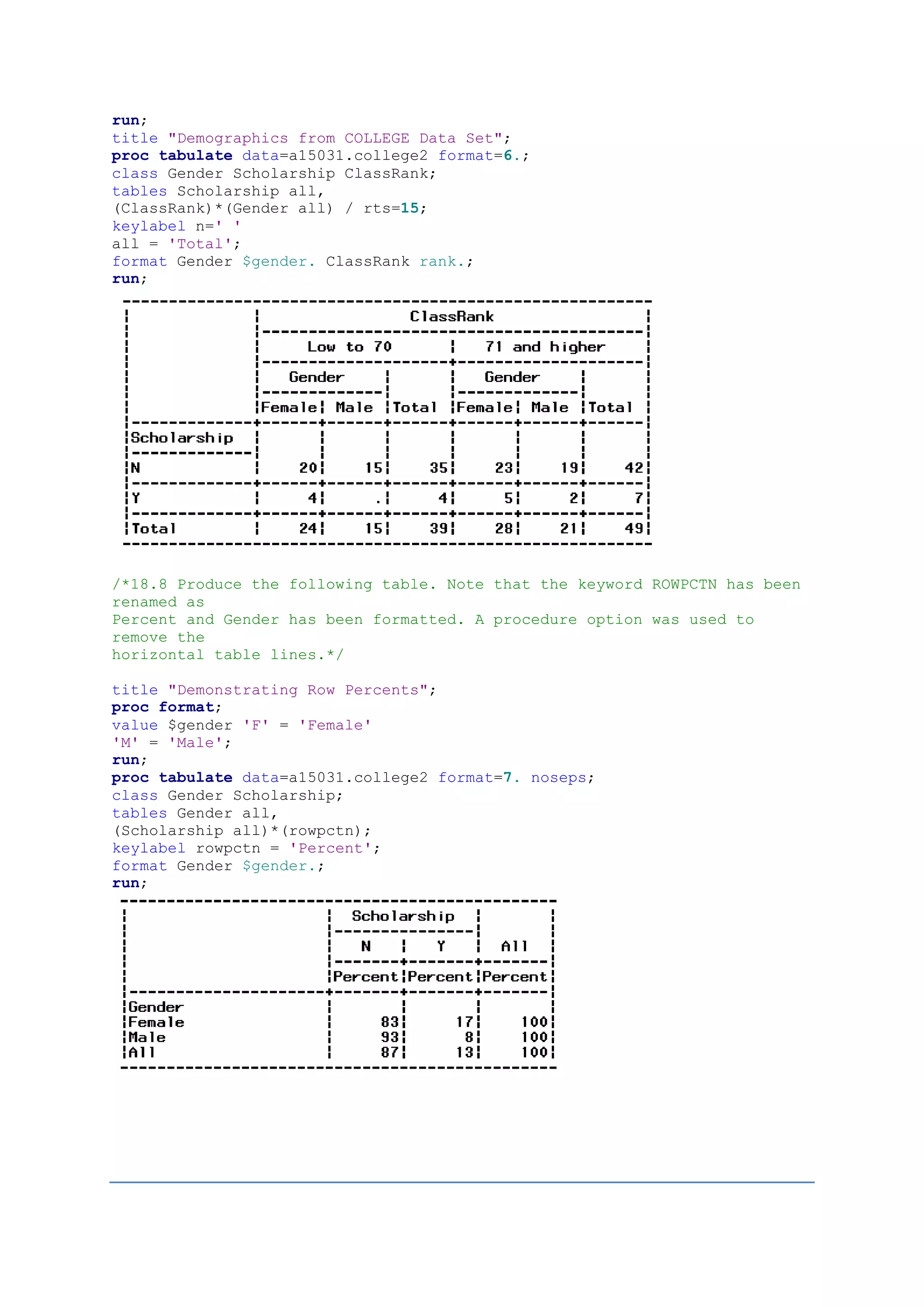

1) The document demonstrates various SAS procedures to analyze and summarize data from multiple SAS data sets, including PROC MEANS, PROC FREQ, PROC TABULATE, PROC GCHART, and PROC GPLOT. 2) Examples include computing statistics by gender and school size using BY and CLASS statements in PROC MEANS, creating frequency tables and cross tabulations in PROC FREQ, producing customized tables using PROC TABULATE, and creating bar charts and scatter plots using PROC GCHART and PROC GPLOT. 3) The document also demonstrates using ODS to produce output files and control formatting and layout of results.
Creating a SAS format library with variables for Gender, SchoolSize, and Scholarship; generating a synthetic dataset for college.
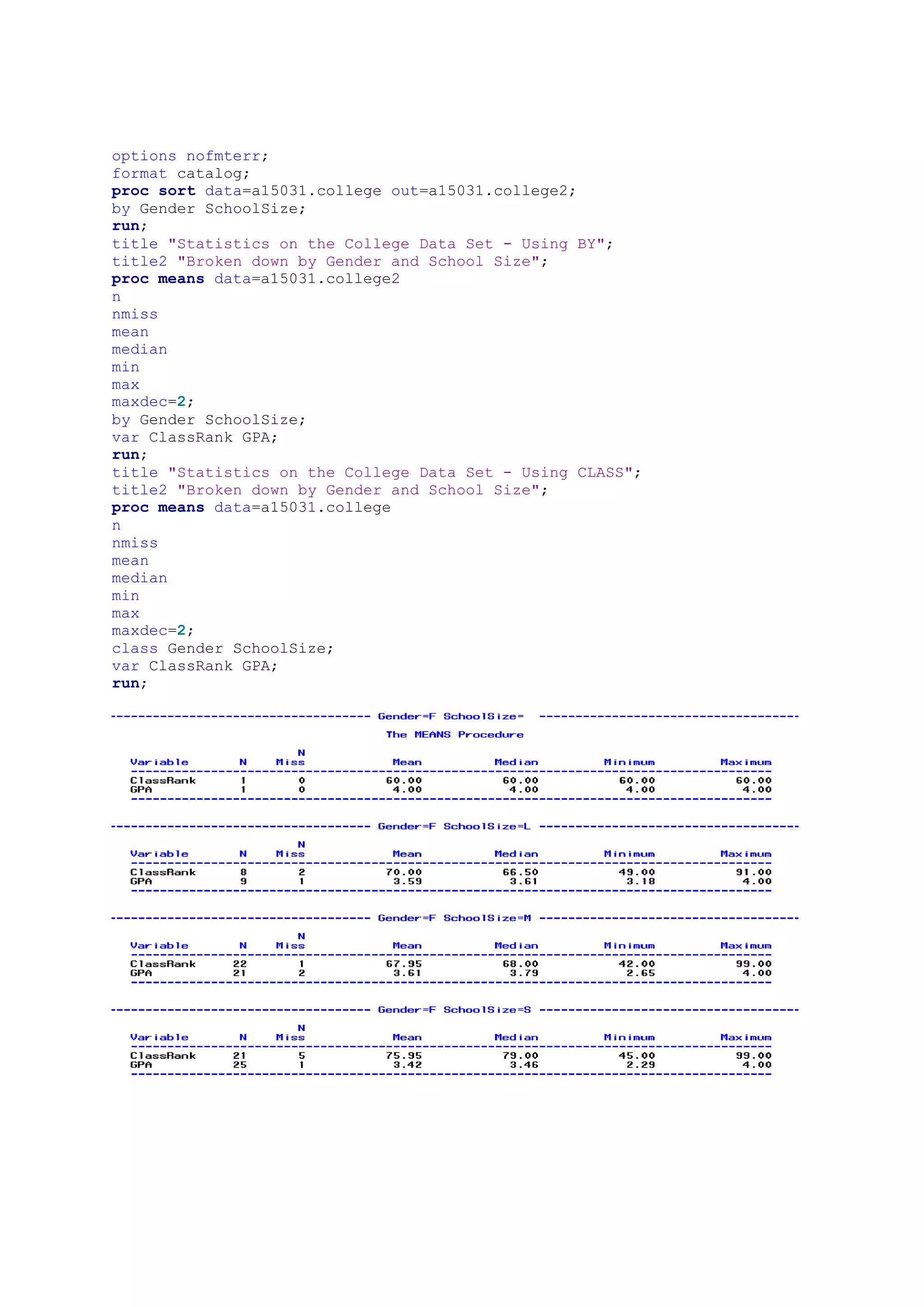
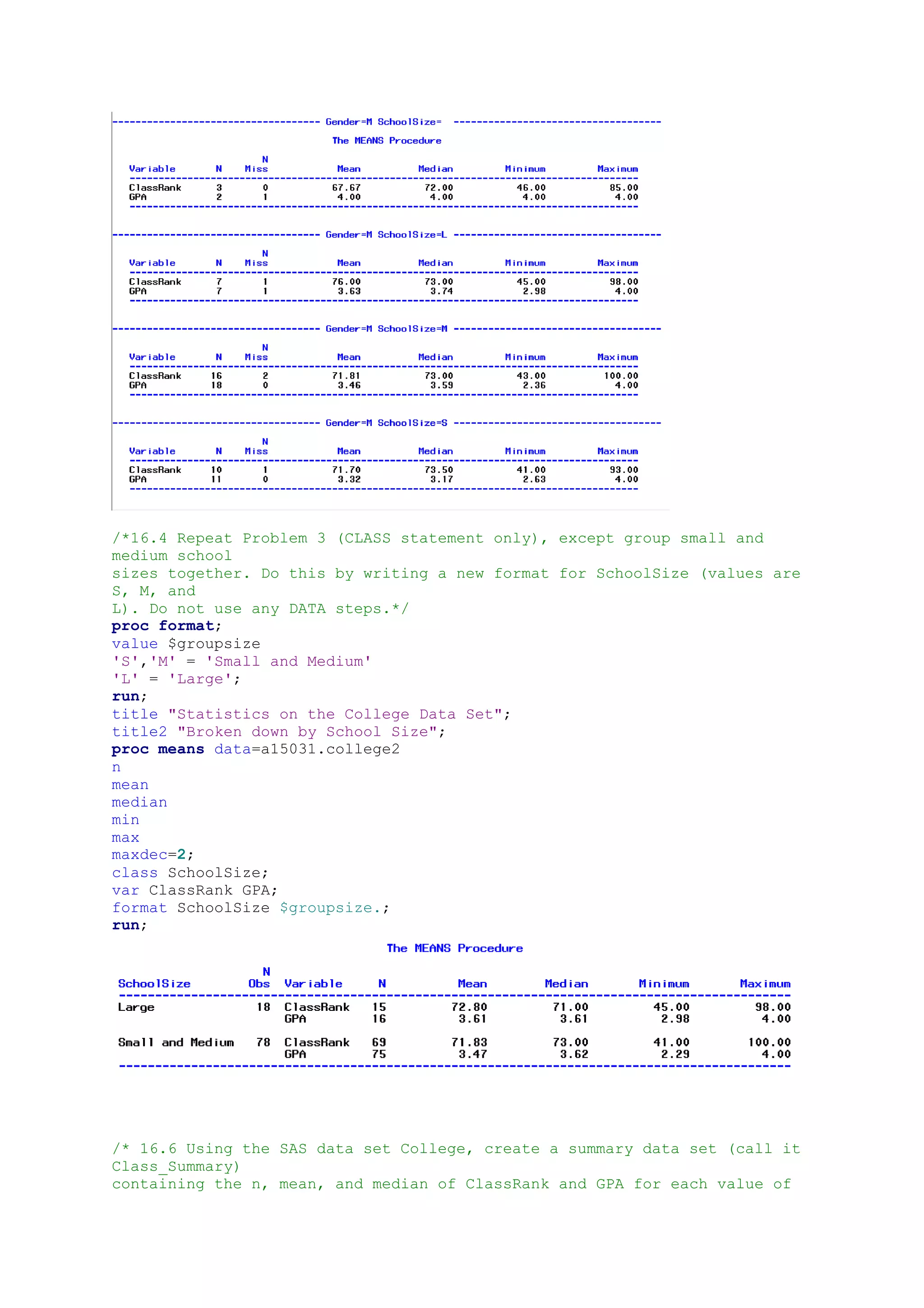
Performing statistical analysis on College data using BY and CLASS statements for ClassRank and GPA by Gender and SchoolSize.
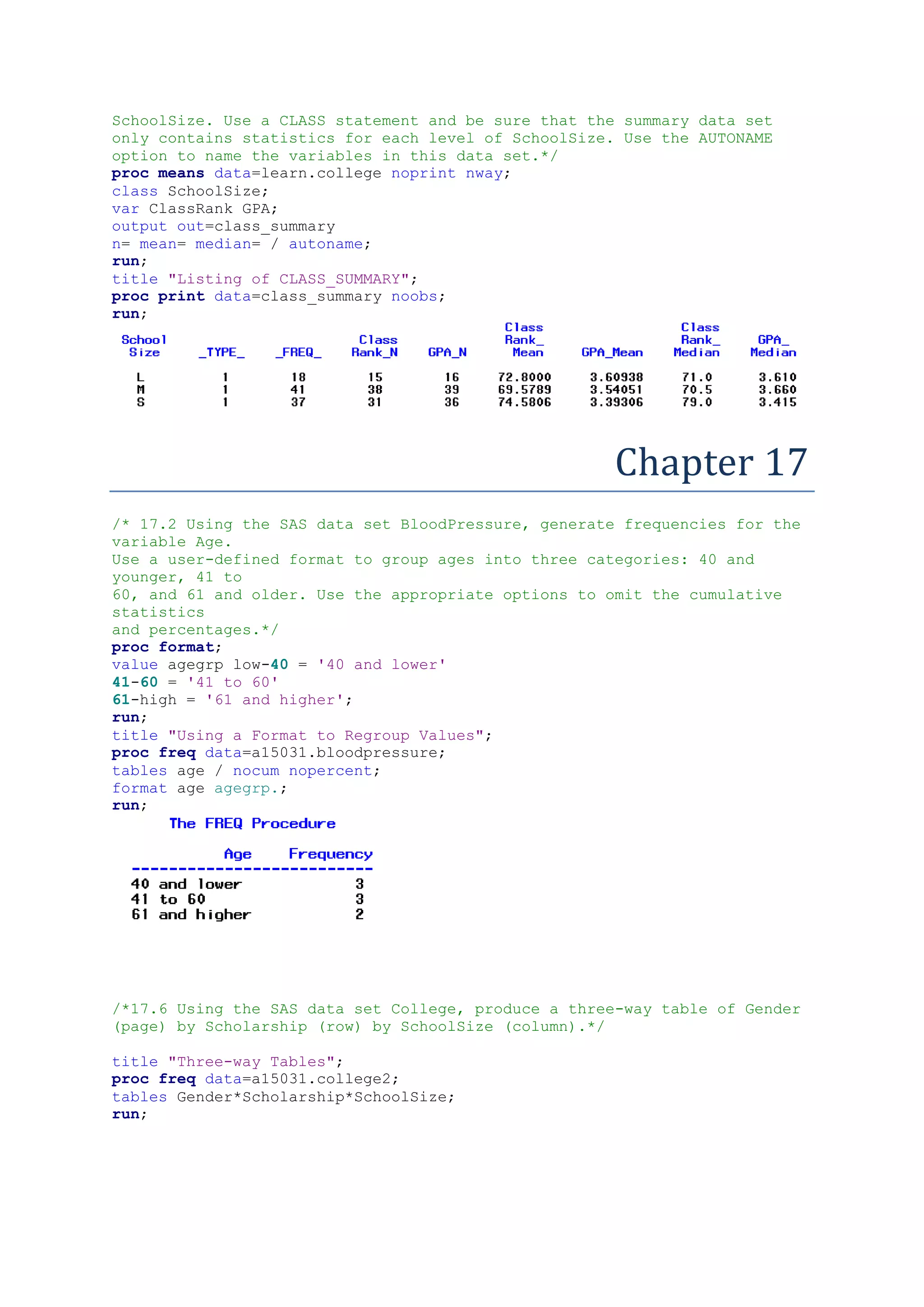
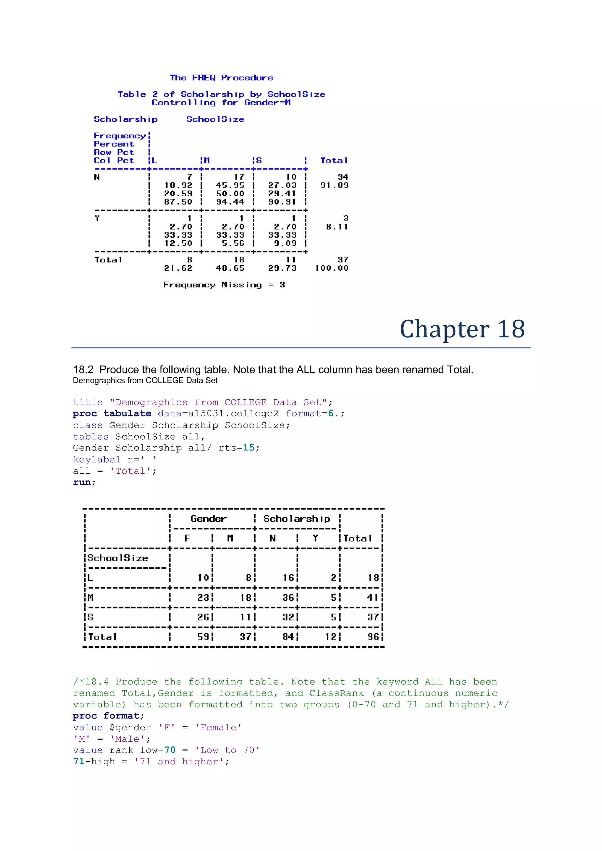
Creating formats to group School sizes; generating summary statistics (mean, median) for ClassRank and GPA based on redefined SchoolSize.Generating frequency distributions for Age, and producing a three-way table of Gender, Scholarship, and SchoolSize.
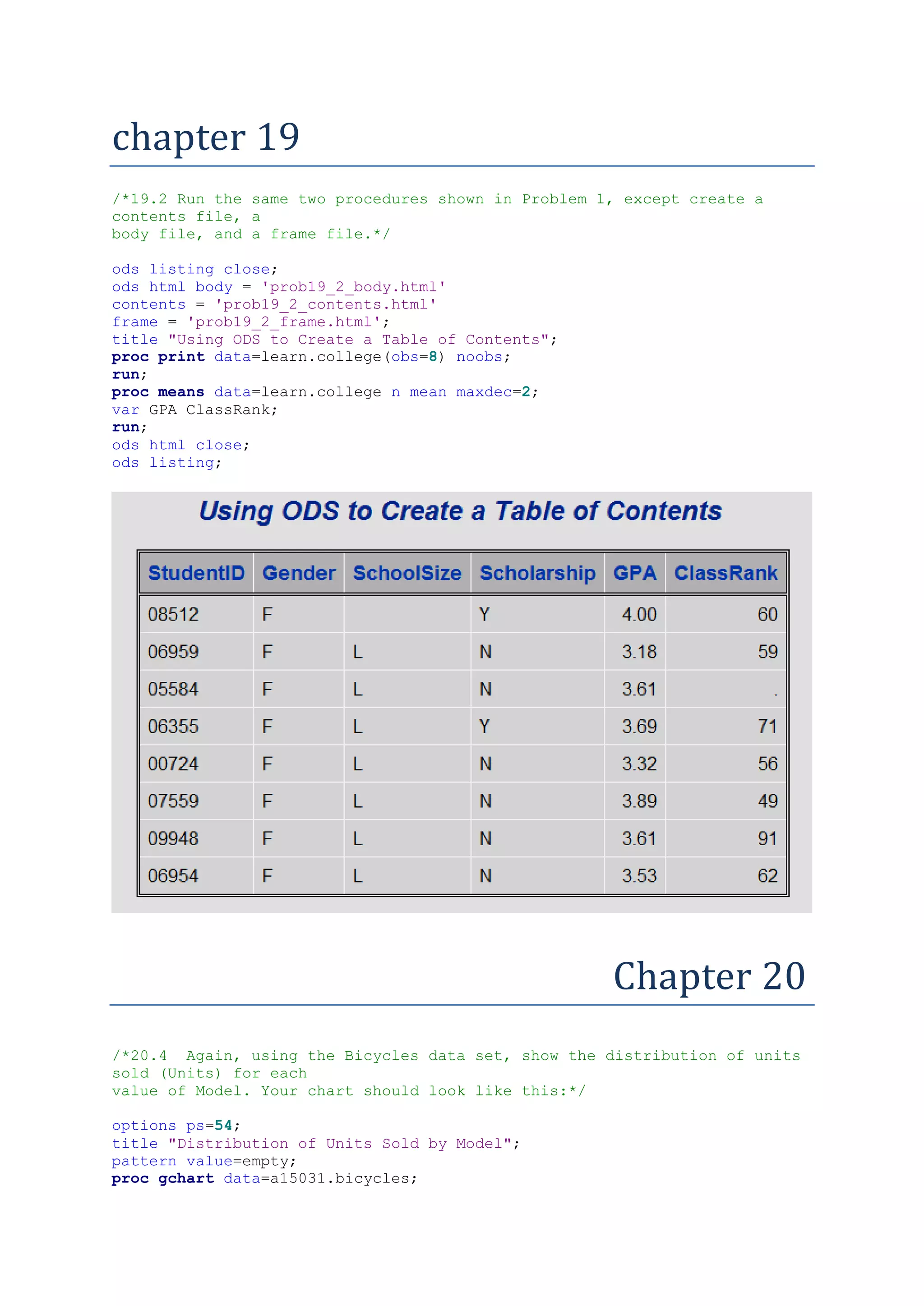
Using ODS to generate HTML files including body, contents, and frame for displaying GPA and ClassRank statistics.
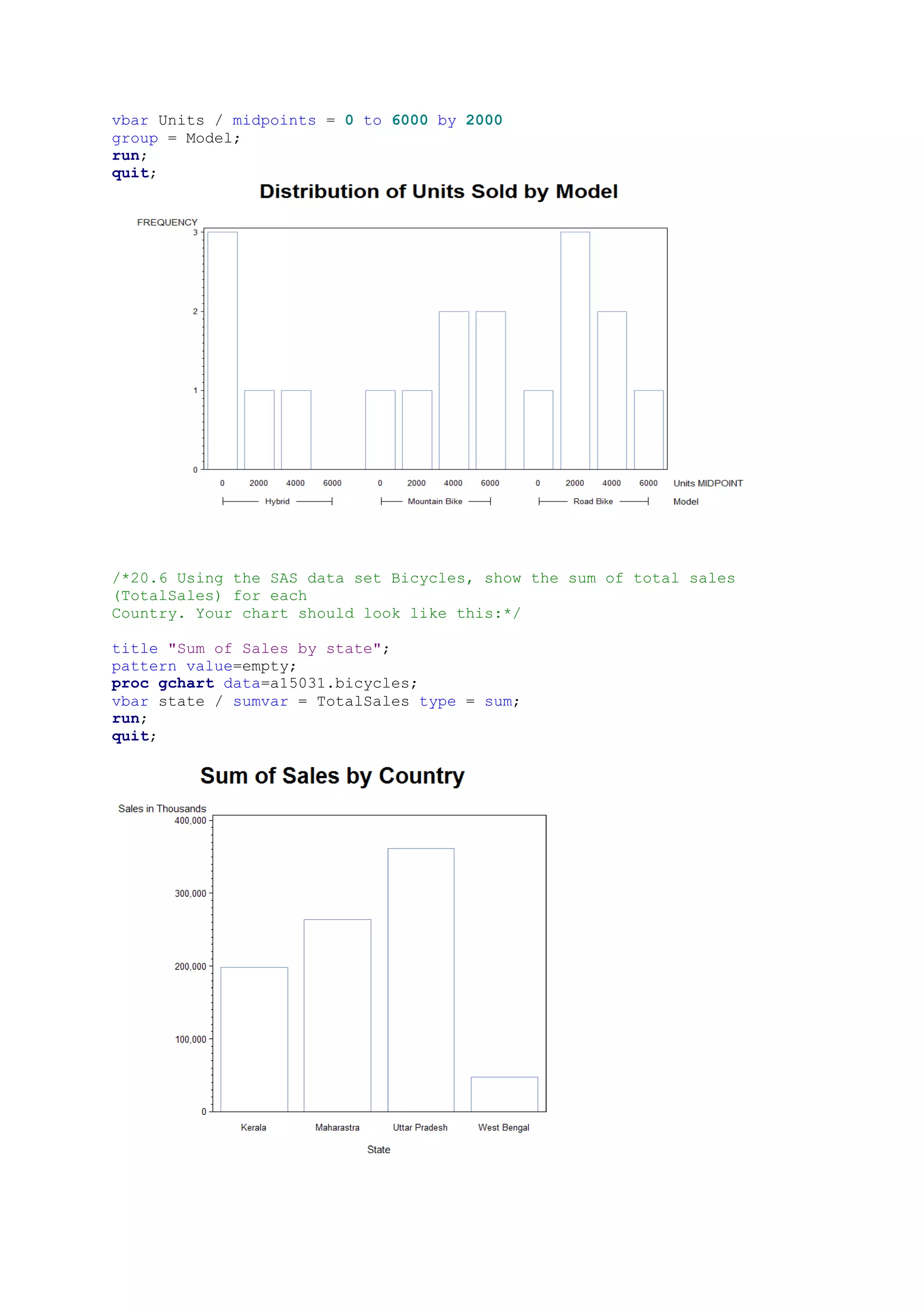
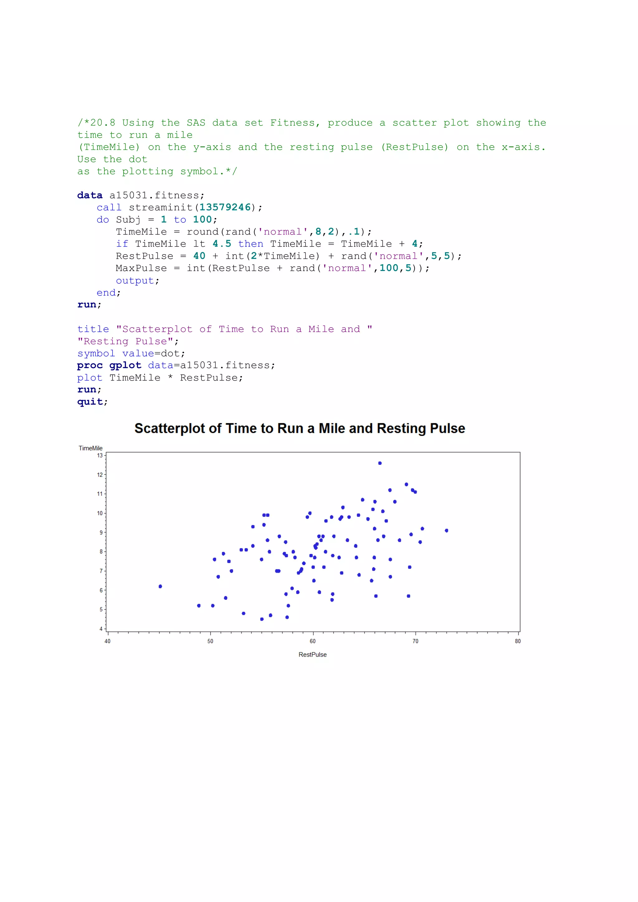
Creating visual representations including bar charts for Units Sold by Model and Total Sales by Country, along with a scatter plot of TimeMile vs. RestPulse.


![[DSC Europe 25] Vid Stimac - Policy Parsimony: Between Oversimplifying and Ov...](https://cdn.slidesharecdn.com/ss_thumbnails/eqlepagzqp2rhg3gbluh-dsc-stimac-251120-251205090438-059e7f54-thumbnail.jpg?width=640&height=640&fit=bounds)


![[DSC Europe 25] Boris Perkovic - Lost in performance.pptx](https://cdn.slidesharecdn.com/ss_thumbnails/uq5hrp7vsuahqkxzifux-1-251204082258-fd2ee09d-thumbnail.jpg?width=640&height=640&fit=bounds)


![[DSC Europe 25] Max Talanov - Non digital NNs.pptx](https://cdn.slidesharecdn.com/ss_thumbnails/wif8tr3gtua74qvtopke-non-digital-nns-251205090438-26b0eea6-thumbnail.jpg?width=640&height=640&fit=bounds)


![[DSC Europe 25] Petar Zivanov - AI meets documents From chatbots to AI-powere...](https://cdn.slidesharecdn.com/ss_thumbnails/xer2bb6nrdc8pdpev0pc-8-251204082258-7c2fa4a1-thumbnail.jpg?width=640&height=640&fit=bounds)


![[DSC Europe 25] Andy Cotgreave - Nothing is new in analytics.pptx](https://cdn.slidesharecdn.com/ss_thumbnails/mba4vzcurvoh5lfrd5zw-6-251205194645-341bbbbe-thumbnail.jpg?width=640&height=640&fit=bounds)
![[DSC Europe 25] Bogdan Daniel Maruneac - AI - It starts with you.pptx](https://cdn.slidesharecdn.com/ss_thumbnails/odov3snhrcqs9hx5ny2n-4-251205085715-f1daacfe-thumbnail.jpg?width=640&height=640&fit=bounds)