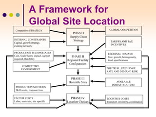
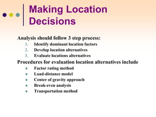
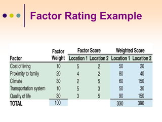
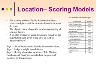
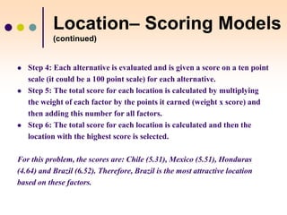
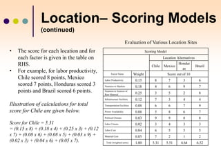
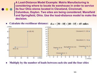
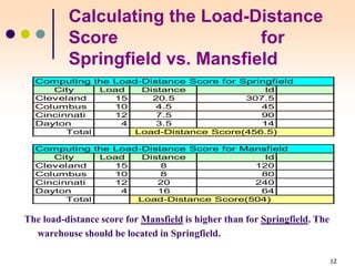
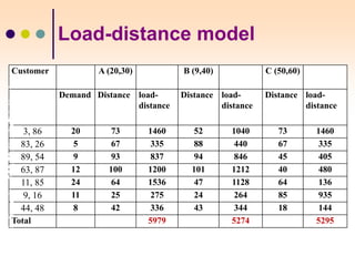
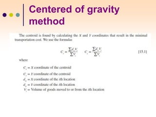
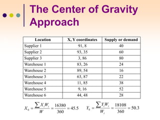
1-1
Copyright ©2013 Pearson Education.
1-1
Copyright ©2013 Pearson Education.
1-1
Copyright ©2013 Pearson Education.
Locating
Logistics
Facilities
5
1-1
Facilities Planning
Facilities are the plant and the office within which P/OM does its work.
There are four main components of facilities planning and they strongly
interact with each other.
 Location of plant, or the branch, or the warehouse.
 Specific structure and site.
 Layout.
 Furniture, lighting, decorative features, and equipment.
In the global world of international production systems, international
markets, and rapid technological transfers, facilities planning requires a
team effort.
A Framework for
Global Site Location
PHASE I
Supply Chain
Strategy
PHASE II
Regional Facility
Configuration
PHASE III
Desirable Sites
PHASE IV
Location Choices
Competitive STRATEGY
INTERNAL CONSTRAINTS
Capital, growth strategy,
existing network
PRODUCTION TECHNOLOGIES
Cost, Scale/Scope impact, support
required, flexibility
COMPETITIVE
ENVIRONMENT
PRODUCTION METHODS
Skill needs, response time
FACTOR COSTS
Labor, materials, site specific
GLOBAL COMPETITION
TARIFFS AND TAX
INCENTIVES
REGIONAL DEMAND
Size, growth, homogeneity,
local specifications
POLITICAL, EXCHANGE
RATE AND DEMAND RISK
AVAILABLE
INFRASTRUCTURE
LOGISTICS COSTS
Transport, inventory, coordination
Service and Number of
Facilities
Number of Facilities
Response
Time
Costs and Number of
Facilities
Costs
Number of facilities
Total SC Inventory
Transportation
Facility costs
No economies of scale in shipment size,
SC covers a larger portion with each facility.
With economies of scale in inbound shipping to retailers.
Making Location
Decisions
Analysis should follow 3 step process:
1. Identify dominant location factors
2. Develop location alternatives
3. Evaluate locations alternatives
Procedures for evaluation location alternatives include
 Factor rating method
 Load-distance model
 Center of gravity approach
 Break-even analysis
 Transportation method
Factor Rating Example
Location– Scoring Models
Factor Name Weight
Labor Productivity 0.15
Nearness to Markets 0.18
Nearness to Sources of
Raw Material
0.25
Infrastructure Facilities 0.12
Transportation Facilities 0.08
Power Availability 0.08
Political Climate 0.03
Labor Unions 0.02
Labor Cost 0.04
Material Cost 0.05
Total 1.00
• The scoring model of facility location provides a
relative weight to each factor that affects the location
decision.
• The objective is to choose the location considering all
relevant factors.
• A six step process for using the scoring model for the
hypothetical data given in the table on RHS is
described below.
Step 1: List all factors that affect the location decisions.
Step 2: Assign a weight to each factor.
Step 3: Identify alternative locations. Chile, Mexico,
Honduras and Brazil are identified are the potential
locations for this problem.
Location Factors and Weights
Location– Scoring Models
(continued)
 Step 4: Each alternative is evaluated and is given a score on a ten point
scale (it could be a 100 point scale) for each alternative.
 Step 5: The total score for each location is calculated by multiplying
the weight of each factor by the points it earned (weight x score) and
then adding this number for all factors.
 Step 6: The total score for each location is calculated and then the
location with the highest score is selected.
For this problem, the scores are: Chile (5.31), Mexico (5.51), Honduras
(4.64) and Brazil (6.52). Therefore, Brazil is the most attractive location
based on these factors.
Location– Scoring Models
(continued)
Scoring Model
Location Alternatives
Chile Mexico
Hondur
as
Brazil
Factor Name Weight Score out of 10
Labor Productivity 0.15 8 7 3 6
Nearness to Markets 0.18 4 6 9 7
Nearness to Sources of
Raw Material 0.25 3 5 2 8
Infrastructure Facilities 0.12 7 3 4 4
Transportation Facilities 0.08 6 6 7 9
Power Availability 0.08 5 8 6 7
Political Climate 0.03 9 9 8 8
Labor Unions 0.02 3 4 3 3
Labor Cost 0.04 6 5 5 5
Material Cost 0.05 7 2 1 2
Total (weighted sums) 1.00 5.31 5.51 4.64 6.52
Evaluation of Various Location Sites
• The score for each location and for
each factor is given in the table on
RHS.
• For example, for labor productivity,
Chile scored 8 points, Mexico
scored 7 points, Honduras scored 3
points and Brazil scored 6 points.
Illustration of calculations for total
score for Chile are given below.
Score for Chile = 5.31
= (0.15 x 8) + (0.18 x 4) + (0.25 x 3) + (0.12
x 7) + (0.08 x 6) + (0.08 x 5) + (0.03 x 9) +
(0.02 x 3) + (0.04 x 6) + (0.05 x 7).
A Load-Distance Model Example: Matrix Manufacturing is
considering where to locate its warehouse in order to service
its four Ohio stores located in Cleveland, Cincinnati,
Columbus, Dayton. Two sites are being considered; Mansfield
and Springfield, Ohio. Use the load-distance model to make the
decision.
 Calculate the rectilinear distance:
 Multiply by the number of loads between each site and the four cities
miles
45
15
40
10
30
dAB 




12
Calculating the Load-Distance
Score for
Springfield vs. Mansfield

The load-distance score for Mansfield is higher than for Springfield. The
warehouse should be located in Springfield.
Computing the Load-Distance Score for Springfield
City Load Distance ld
Cleveland 15 20.5 307.5
Columbus 10 4.5 45
Cincinnati 12 7.5 90
Dayton 4 3.5 14
Total Load-Distance Score(456.5)
Computing the Load-Distance Score for Mansfield
City Load Distance ld
Cleveland 15 8 120
Columbus 10 8 80
Cincinnati 12 20 240
Dayton 4 16 64
Total Load-Distance Score(504)
WS 2004/5
Load-distance model
Customer A (20,30) B (9,40) C (50,60)
Demand Distance load-
distance
Distance load-
distance
Distance load-
distance
3, 86 20 73 1460 52 1040 73 1460
83, 26 5 67 335 88 440 67 335
89, 54 9 93 837 94 846 45 405
63, 87 12 100 1200 101 1212 40 480
11, 85 24 64 1536 47 1128 64 136
9, 16 11 25 275 24 264 85 935
44, 48 8 42 336 43 344 18 144
Total 5979 5274 5295
Quản
trị
chuỗi
cung
ứng-
PGS.
TS.
Nguyễn
Phúc
Nguyên
Centered of gravity
method
The Center of Gravity
Approach
 This approach requires that the analyst find the center of gravity of the
geographic area being considered
 Computing the Center of Gravity for Matrix Manufacturing
 Is there another possible warehouse location closer to the C.G. that should be
considered?? Why?
10.6
41
436
l
Y
l
Y
;
7.9
41
325
l
X
l
X
i
i
i
c.g.
i
i
i
c.g. 









Computing the Center of Gravity for Matrix Manufacturing
Coordinates Load
Location (X,Y) (li) lixi liyi
Cleveland (11,22) 15 165 330
Columbus (10,7) 10 165 70
Cincinnati (4,1) 12 165 12
Dayton (3,6) 4 165 24
Total 41 325 436
WS 2004/5
The Center of Gravity
Approach
Location X, Y coordinates Supply or demand
Supplier 1 91, 8 40
Supplier 2 93, 35 60
Supplier 3 3, 86 80
Warehouse 1 83, 26 24
Warehouse 2 89, 54 16
Warehouse 3 63, 87 22
Warehouse 4 11, 85 38
Warehouse 5 9, 16 52
Warehouse 6 44, 48 28
5
.
45
360
16380
0 



W
W
X
X
i
i
3
.
50
360
18108
0 



i
i
i
W
W
Y
Y
Quản
trị
chuỗi
cung
ứng-
PGS.
TS.
Nguyễn
Phúc
Nguyên
WS 2004/5
The Center of Gravity
Approach
0
10
20
30
40
50
60
70
80
90
100
0 10 20 30 40 50 60 70 80 90 100
Nhà cung cấp
Nhà kho
Trọng tâm
Quản
trị
chuỗi
cung
ứng-
PGS.
TS.
Nguyễn
Phúc
Nguyên
Location Decisions Using
Breakeven Models
How many units of throughput need to be sold in order to recover costs (variable
and fixed) and breakeven?
Variable (Direct) Costs
Variable (direct) costs per unit are the costs of input resources that tend to be fully
chargeable and directly attributable to each unit of the product.
Total variable costs, TVC = C*Q, where C is variable cost per unit and Q is the
number of units produced.
Fixed (indirect) Costs
Fixed costs have to be paid, whether one unit is made or thousands.
These costs are bundled together as overhead costs.
Revenue
Total revenue, TR = P*Q, is the volume Q multiplied by the price per unit P.
Location Decisions Using
Breakeven Models (continued)
Example:
 Musuk Spices Company (MSC), Delhi, India, plans to set up a new
plant at one of the following two locations: Bhopal and Agra in India.
 The fixed costs per year will be $ 450,000 and $ 300,000 per year for
Bhopal and Agra respectively.
 The variable costs per pound are expected to be $ 10/lb. for Bhopal
and $ 14/lb. for Agra respectively.
 The selling price is expected to be $ 30/lb.
 Breakeven Point (BEP) = Fixed Cost/(Selling Price – Variable Cost)
 BEP (Bhopal) = 450,000/(30-10) = 22,500 lbs.
 BEP (Agra) = 300,000/(30- 14) = 18,750 lbs.
Location Decisions Using
Breakeven Models (continued)
 Bhopal will generate profits only if the volume of demand is more than
22,500 lbs.
 Agra will start generating profits if the volume is more than 18,750.
 If demand is likely to be about 20,000, then Agra is chosen.
Say demand will exceed 25,000, which plant should be selected?
 Find the point of indifference.
 Find revenue if Q lbs. of spices are produced and sold by each plant.
Revenue (Bhopal) = Q (30-10) - 450,000 = 20 Q - 450,000
Revenue (Agra) = Q (30-14) - 300,000 = 16 Q - 300,000
Equate the two revenues to find the point of indifference – the value of Q.
Q = (450,000 – 300,000)/ (20-16) = 150,000/4 = 37,500.
Location Decisions Using
Breakeven Models (continued)
The indifference point Q = 37,500.
Plant at Bhopal is more desirable if the expected volume of sales is more
than 37,500.
If the expected sales are less than 37,500 then Agra is more desirable.
Either one of them can be chosen if the sales are exactly 37,500.
Forecasts have an important role to play in this example.
WS 2004/5
Network models
 Single median problem: Finding one note to serve the others
Quản
trị
chuỗi
cung
ứng-
PGS.
TS.
Nguyễn
Phúc
Nguyên
WS 2004/5
Network models
 Single median problem
Demand A B C D E F G H
A 10 0 15 22 24 31 28 32 36
B 15 15 0 8 9 16 14 17 21
C 25 22 8 0 17 12 6 25 17
D 20 24 9 17 0 7 13 8 12
E 20 31 16 12 7 0 6 15 5
F 10 28 14 6 13 6 0 21 11
G 10 32 17 25 8 15 21 0 14
H 15 36 21 17 12 5 11 14 0
TC 125 3015 1475 1485 1330 1275 1395 2080 1690
Quản
trị
chuỗi
cung
ứng-
PGS.
TS.
Nguyễn
Phúc
Nguyên
WS 2004/5
Network models
 Covering problem: Focusing on service level
Quản
trị
chuỗi
cung
ứng-
PGS.
TS.
Nguyễn
Phúc
Nguyên
WS 2004/5
Covering problem
Distance matrix
A B C D E F G H I J
A 0 10 24 10 29 29 25 20 35 32
B 10 0 14 20 19 19 15 30 25 22
C 24 14 0 15 11 5 15 25 11 14
D 10 20 15 0 26 20 30 10 25 29
E 29 19 11 26 0 6 4 23 8 3
F 29 19 5 20 6 0 10 21 6 9
G 25 15 15 30 4 10 0 27 12 7
H 20 30 25 10 23 21 27 0 15 20
I 35 25 11 25 8 6 12 15 0 5
J 32 22 14 29 3 9 7 20 5 0
Maximum 35 30 25 30 29 29 30 30 35 32
Single location C
Maximum time 25
Quản
trị
chuỗi
cung
ứng-
PGS.
TS.
Nguyễn
Phúc
Nguyên
WS 2004/5
Covering problem: 15
minutes service level
A B C D E F G H I J
A 0 10 10
B 10 0 14 15
C 14 0 15 11 5 15 11 14
D 10 15 0 10
E 11 0 6 4 8 3
F 5 6 0 10 6 9
G 15 15 4 10 0 12 7
H 10 0 15
I 11 8 6 12 15 0 5
J 14 3 9 7 5 0
Tối đa
10 15 15 15 11 9 15 15 15 14
Quản
trị
chuỗi
cung
ứng-
PGS.
TS.
Nguyễn
Phúc
Nguyên
WS 2004/5
0 / 27
Covering problem: 15
minutes service level
Alternatives
A & I C & D G & D
A I C D G D
A 0 10 10
B 10 14 15
C 11 0 15
D 10 0 0
E 8 11 4
F 6 5 10
G 12 15 0
H 15 10 10
I 0 11 12
J 5 14 7
Maximum time 10 15 15 10 15 15
Average time 7.7 9 8.3
Quản
trị
chuỗi
cung
ứng-
PGS.
TS.
Nguyễn
Phúc
Nguyên
Mathematical model
 Information:
 There are two factories P1 và P2, production cost of two facoties
are same, Capacity of P2 : 60.000, P1 : 150.000 (products)
 There are two warehouses W1 and W2,
 There are three markets C1, C2, C3,
 Requirement: Finding the optimal solution
P1 P2 C1 C2 C3
W1 0 4 3 4 5
W2 5 2 2 1 2
Capacity unlimit 60.000 50.000 100.000 50.000
WS 2004/5
Mathematical model
 Optimal solution:
 Cost for delivering product from plant to warehouse:
: Cost from plant i to warehouse j
• : Total volume from plant i to warehouse j
 Cost for delivering product from warehouse to market:
 : Cosst from warehouse j to market k
• : Total vomule from warehouse j to market k
 )
,
( j
i
ij W
P
f
c
ij
c
)
,
( j
i W
P
f
 )
,
( k
j
jk C
W
f
c
ik
c
)
,
( k
j C
W
f
Quản
trị
chuỗi
cung
ứng-
PGS.
TS.
Nguyễn
Phúc
Nguyên
WS 2004/5
0 / 30
Mathematical model
 Constraints:
    000
.
60
,
, 2
2
1
2 
 W
P
f
W
P
f
         
3
1
2
1
1
1
1
2
1
1 ,
,
,
,
, C
W
f
C
W
f
C
W
f
W
P
f
W
P
f 



         
3
2
2
2
1
2
2
2
2
1 ,
,
,
,
, C
W
f
C
W
f
C
W
f
W
P
f
W
P
f 



    000
.
50
,
, 1
2
1
1 
 C
W
f
C
W
f
    000
.
100
,
, 2
2
2
1 
 C
W
f
C
W
f
    000
.
50
,
, 3
2
3
1 
 C
W
f
C
W
f
1
2
3
4
5
6
7     0
,
;
, 
k
j
j
i C
W
f
W
P
f
Quản
trị
chuỗi
cung
ứng-
PGS.
TS.
Nguyễn
Phúc
Nguyên
WS 2004/5
Mathematical model
 Optimal solution:
 Total cost: 740.000 $
P1 P2 C1 C2 C3
W1 140.000 0 50.000 40.000 50.000
W2 0 60.000 0 60.000 0
Quản
trị
chuỗi
cung
ứng-
PGS.
TS.
Nguyễn
Phúc
Nguyên

Chap 5.ppt

  • 1.
    1-1 Copyright ©2013 PearsonEducation. Copyright ©2013 Pearson Education. Copyright ©2013 Pearson Education. 1-1 Copyright ©2013 Pearson Education. 1-1 Copyright ©2013 Pearson Education. Locating Logistics Facilities 5 1-1
  • 2.
    Facilities Planning Facilities arethe plant and the office within which P/OM does its work. There are four main components of facilities planning and they strongly interact with each other.  Location of plant, or the branch, or the warehouse.  Specific structure and site.  Layout.  Furniture, lighting, decorative features, and equipment. In the global world of international production systems, international markets, and rapid technological transfers, facilities planning requires a team effort.
  • 3.
    A Framework for GlobalSite Location PHASE I Supply Chain Strategy PHASE II Regional Facility Configuration PHASE III Desirable Sites PHASE IV Location Choices Competitive STRATEGY INTERNAL CONSTRAINTS Capital, growth strategy, existing network PRODUCTION TECHNOLOGIES Cost, Scale/Scope impact, support required, flexibility COMPETITIVE ENVIRONMENT PRODUCTION METHODS Skill needs, response time FACTOR COSTS Labor, materials, site specific GLOBAL COMPETITION TARIFFS AND TAX INCENTIVES REGIONAL DEMAND Size, growth, homogeneity, local specifications POLITICAL, EXCHANGE RATE AND DEMAND RISK AVAILABLE INFRASTRUCTURE LOGISTICS COSTS Transport, inventory, coordination
  • 4.
    Service and Numberof Facilities Number of Facilities Response Time
  • 5.
    Costs and Numberof Facilities Costs Number of facilities Total SC Inventory Transportation Facility costs No economies of scale in shipment size, SC covers a larger portion with each facility. With economies of scale in inbound shipping to retailers.
  • 6.
    Making Location Decisions Analysis shouldfollow 3 step process: 1. Identify dominant location factors 2. Develop location alternatives 3. Evaluate locations alternatives Procedures for evaluation location alternatives include  Factor rating method  Load-distance model  Center of gravity approach  Break-even analysis  Transportation method
  • 7.
  • 8.
    Location– Scoring Models FactorName Weight Labor Productivity 0.15 Nearness to Markets 0.18 Nearness to Sources of Raw Material 0.25 Infrastructure Facilities 0.12 Transportation Facilities 0.08 Power Availability 0.08 Political Climate 0.03 Labor Unions 0.02 Labor Cost 0.04 Material Cost 0.05 Total 1.00 • The scoring model of facility location provides a relative weight to each factor that affects the location decision. • The objective is to choose the location considering all relevant factors. • A six step process for using the scoring model for the hypothetical data given in the table on RHS is described below. Step 1: List all factors that affect the location decisions. Step 2: Assign a weight to each factor. Step 3: Identify alternative locations. Chile, Mexico, Honduras and Brazil are identified are the potential locations for this problem. Location Factors and Weights
  • 9.
    Location– Scoring Models (continued) Step 4: Each alternative is evaluated and is given a score on a ten point scale (it could be a 100 point scale) for each alternative.  Step 5: The total score for each location is calculated by multiplying the weight of each factor by the points it earned (weight x score) and then adding this number for all factors.  Step 6: The total score for each location is calculated and then the location with the highest score is selected. For this problem, the scores are: Chile (5.31), Mexico (5.51), Honduras (4.64) and Brazil (6.52). Therefore, Brazil is the most attractive location based on these factors.
  • 10.
    Location– Scoring Models (continued) ScoringModel Location Alternatives Chile Mexico Hondur as Brazil Factor Name Weight Score out of 10 Labor Productivity 0.15 8 7 3 6 Nearness to Markets 0.18 4 6 9 7 Nearness to Sources of Raw Material 0.25 3 5 2 8 Infrastructure Facilities 0.12 7 3 4 4 Transportation Facilities 0.08 6 6 7 9 Power Availability 0.08 5 8 6 7 Political Climate 0.03 9 9 8 8 Labor Unions 0.02 3 4 3 3 Labor Cost 0.04 6 5 5 5 Material Cost 0.05 7 2 1 2 Total (weighted sums) 1.00 5.31 5.51 4.64 6.52 Evaluation of Various Location Sites • The score for each location and for each factor is given in the table on RHS. • For example, for labor productivity, Chile scored 8 points, Mexico scored 7 points, Honduras scored 3 points and Brazil scored 6 points. Illustration of calculations for total score for Chile are given below. Score for Chile = 5.31 = (0.15 x 8) + (0.18 x 4) + (0.25 x 3) + (0.12 x 7) + (0.08 x 6) + (0.08 x 5) + (0.03 x 9) + (0.02 x 3) + (0.04 x 6) + (0.05 x 7).
  • 11.
    A Load-Distance ModelExample: Matrix Manufacturing is considering where to locate its warehouse in order to service its four Ohio stores located in Cleveland, Cincinnati, Columbus, Dayton. Two sites are being considered; Mansfield and Springfield, Ohio. Use the load-distance model to make the decision.  Calculate the rectilinear distance:  Multiply by the number of loads between each site and the four cities miles 45 15 40 10 30 dAB     
  • 12.
    12 Calculating the Load-Distance Scorefor Springfield vs. Mansfield  The load-distance score for Mansfield is higher than for Springfield. The warehouse should be located in Springfield. Computing the Load-Distance Score for Springfield City Load Distance ld Cleveland 15 20.5 307.5 Columbus 10 4.5 45 Cincinnati 12 7.5 90 Dayton 4 3.5 14 Total Load-Distance Score(456.5) Computing the Load-Distance Score for Mansfield City Load Distance ld Cleveland 15 8 120 Columbus 10 8 80 Cincinnati 12 20 240 Dayton 4 16 64 Total Load-Distance Score(504)
  • 13.
    WS 2004/5 Load-distance model CustomerA (20,30) B (9,40) C (50,60) Demand Distance load- distance Distance load- distance Distance load- distance 3, 86 20 73 1460 52 1040 73 1460 83, 26 5 67 335 88 440 67 335 89, 54 9 93 837 94 846 45 405 63, 87 12 100 1200 101 1212 40 480 11, 85 24 64 1536 47 1128 64 136 9, 16 11 25 275 24 264 85 935 44, 48 8 42 336 43 344 18 144 Total 5979 5274 5295 Quản trị chuỗi cung ứng- PGS. TS. Nguyễn Phúc Nguyên
  • 14.
  • 15.
    The Center ofGravity Approach  This approach requires that the analyst find the center of gravity of the geographic area being considered  Computing the Center of Gravity for Matrix Manufacturing  Is there another possible warehouse location closer to the C.G. that should be considered?? Why? 10.6 41 436 l Y l Y ; 7.9 41 325 l X l X i i i c.g. i i i c.g.           Computing the Center of Gravity for Matrix Manufacturing Coordinates Load Location (X,Y) (li) lixi liyi Cleveland (11,22) 15 165 330 Columbus (10,7) 10 165 70 Cincinnati (4,1) 12 165 12 Dayton (3,6) 4 165 24 Total 41 325 436
  • 16.
    WS 2004/5 The Centerof Gravity Approach Location X, Y coordinates Supply or demand Supplier 1 91, 8 40 Supplier 2 93, 35 60 Supplier 3 3, 86 80 Warehouse 1 83, 26 24 Warehouse 2 89, 54 16 Warehouse 3 63, 87 22 Warehouse 4 11, 85 38 Warehouse 5 9, 16 52 Warehouse 6 44, 48 28 5 . 45 360 16380 0     W W X X i i 3 . 50 360 18108 0     i i i W W Y Y Quản trị chuỗi cung ứng- PGS. TS. Nguyễn Phúc Nguyên
  • 17.
    WS 2004/5 The Centerof Gravity Approach 0 10 20 30 40 50 60 70 80 90 100 0 10 20 30 40 50 60 70 80 90 100 Nhà cung cấp Nhà kho Trọng tâm Quản trị chuỗi cung ứng- PGS. TS. Nguyễn Phúc Nguyên
  • 18.
    Location Decisions Using BreakevenModels How many units of throughput need to be sold in order to recover costs (variable and fixed) and breakeven? Variable (Direct) Costs Variable (direct) costs per unit are the costs of input resources that tend to be fully chargeable and directly attributable to each unit of the product. Total variable costs, TVC = C*Q, where C is variable cost per unit and Q is the number of units produced. Fixed (indirect) Costs Fixed costs have to be paid, whether one unit is made or thousands. These costs are bundled together as overhead costs. Revenue Total revenue, TR = P*Q, is the volume Q multiplied by the price per unit P.
  • 19.
    Location Decisions Using BreakevenModels (continued) Example:  Musuk Spices Company (MSC), Delhi, India, plans to set up a new plant at one of the following two locations: Bhopal and Agra in India.  The fixed costs per year will be $ 450,000 and $ 300,000 per year for Bhopal and Agra respectively.  The variable costs per pound are expected to be $ 10/lb. for Bhopal and $ 14/lb. for Agra respectively.  The selling price is expected to be $ 30/lb.  Breakeven Point (BEP) = Fixed Cost/(Selling Price – Variable Cost)  BEP (Bhopal) = 450,000/(30-10) = 22,500 lbs.  BEP (Agra) = 300,000/(30- 14) = 18,750 lbs.
  • 20.
    Location Decisions Using BreakevenModels (continued)  Bhopal will generate profits only if the volume of demand is more than 22,500 lbs.  Agra will start generating profits if the volume is more than 18,750.  If demand is likely to be about 20,000, then Agra is chosen. Say demand will exceed 25,000, which plant should be selected?  Find the point of indifference.  Find revenue if Q lbs. of spices are produced and sold by each plant. Revenue (Bhopal) = Q (30-10) - 450,000 = 20 Q - 450,000 Revenue (Agra) = Q (30-14) - 300,000 = 16 Q - 300,000 Equate the two revenues to find the point of indifference – the value of Q. Q = (450,000 – 300,000)/ (20-16) = 150,000/4 = 37,500.
  • 21.
    Location Decisions Using BreakevenModels (continued) The indifference point Q = 37,500. Plant at Bhopal is more desirable if the expected volume of sales is more than 37,500. If the expected sales are less than 37,500 then Agra is more desirable. Either one of them can be chosen if the sales are exactly 37,500. Forecasts have an important role to play in this example.
  • 22.
    WS 2004/5 Network models Single median problem: Finding one note to serve the others Quản trị chuỗi cung ứng- PGS. TS. Nguyễn Phúc Nguyên
  • 23.
    WS 2004/5 Network models Single median problem Demand A B C D E F G H A 10 0 15 22 24 31 28 32 36 B 15 15 0 8 9 16 14 17 21 C 25 22 8 0 17 12 6 25 17 D 20 24 9 17 0 7 13 8 12 E 20 31 16 12 7 0 6 15 5 F 10 28 14 6 13 6 0 21 11 G 10 32 17 25 8 15 21 0 14 H 15 36 21 17 12 5 11 14 0 TC 125 3015 1475 1485 1330 1275 1395 2080 1690 Quản trị chuỗi cung ứng- PGS. TS. Nguyễn Phúc Nguyên
  • 24.
    WS 2004/5 Network models Covering problem: Focusing on service level Quản trị chuỗi cung ứng- PGS. TS. Nguyễn Phúc Nguyên
  • 25.
    WS 2004/5 Covering problem Distancematrix A B C D E F G H I J A 0 10 24 10 29 29 25 20 35 32 B 10 0 14 20 19 19 15 30 25 22 C 24 14 0 15 11 5 15 25 11 14 D 10 20 15 0 26 20 30 10 25 29 E 29 19 11 26 0 6 4 23 8 3 F 29 19 5 20 6 0 10 21 6 9 G 25 15 15 30 4 10 0 27 12 7 H 20 30 25 10 23 21 27 0 15 20 I 35 25 11 25 8 6 12 15 0 5 J 32 22 14 29 3 9 7 20 5 0 Maximum 35 30 25 30 29 29 30 30 35 32 Single location C Maximum time 25 Quản trị chuỗi cung ứng- PGS. TS. Nguyễn Phúc Nguyên
  • 26.
    WS 2004/5 Covering problem:15 minutes service level A B C D E F G H I J A 0 10 10 B 10 0 14 15 C 14 0 15 11 5 15 11 14 D 10 15 0 10 E 11 0 6 4 8 3 F 5 6 0 10 6 9 G 15 15 4 10 0 12 7 H 10 0 15 I 11 8 6 12 15 0 5 J 14 3 9 7 5 0 Tối đa 10 15 15 15 11 9 15 15 15 14 Quản trị chuỗi cung ứng- PGS. TS. Nguyễn Phúc Nguyên
  • 27.
    WS 2004/5 0 /27 Covering problem: 15 minutes service level Alternatives A & I C & D G & D A I C D G D A 0 10 10 B 10 14 15 C 11 0 15 D 10 0 0 E 8 11 4 F 6 5 10 G 12 15 0 H 15 10 10 I 0 11 12 J 5 14 7 Maximum time 10 15 15 10 15 15 Average time 7.7 9 8.3 Quản trị chuỗi cung ứng- PGS. TS. Nguyễn Phúc Nguyên
  • 28.
    Mathematical model  Information: There are two factories P1 và P2, production cost of two facoties are same, Capacity of P2 : 60.000, P1 : 150.000 (products)  There are two warehouses W1 and W2,  There are three markets C1, C2, C3,  Requirement: Finding the optimal solution P1 P2 C1 C2 C3 W1 0 4 3 4 5 W2 5 2 2 1 2 Capacity unlimit 60.000 50.000 100.000 50.000
  • 29.
    WS 2004/5 Mathematical model Optimal solution:  Cost for delivering product from plant to warehouse: : Cost from plant i to warehouse j • : Total volume from plant i to warehouse j  Cost for delivering product from warehouse to market:  : Cosst from warehouse j to market k • : Total vomule from warehouse j to market k  ) , ( j i ij W P f c ij c ) , ( j i W P f  ) , ( k j jk C W f c ik c ) , ( k j C W f Quản trị chuỗi cung ứng- PGS. TS. Nguyễn Phúc Nguyên
  • 30.
    WS 2004/5 0 /30 Mathematical model  Constraints:     000 . 60 , , 2 2 1 2   W P f W P f           3 1 2 1 1 1 1 2 1 1 , , , , , C W f C W f C W f W P f W P f               3 2 2 2 1 2 2 2 2 1 , , , , , C W f C W f C W f W P f W P f         000 . 50 , , 1 2 1 1   C W f C W f     000 . 100 , , 2 2 2 1   C W f C W f     000 . 50 , , 3 2 3 1   C W f C W f 1 2 3 4 5 6 7     0 , ; ,  k j j i C W f W P f Quản trị chuỗi cung ứng- PGS. TS. Nguyễn Phúc Nguyên
  • 31.
    WS 2004/5 Mathematical model Optimal solution:  Total cost: 740.000 $ P1 P2 C1 C2 C3 W1 140.000 0 50.000 40.000 50.000 W2 0 60.000 0 60.000 0 Quản trị chuỗi cung ứng- PGS. TS. Nguyễn Phúc Nguyên