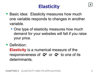
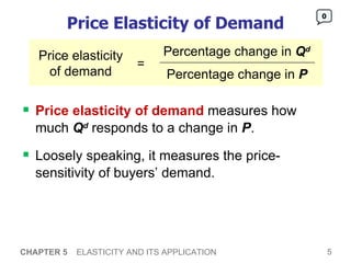
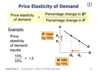
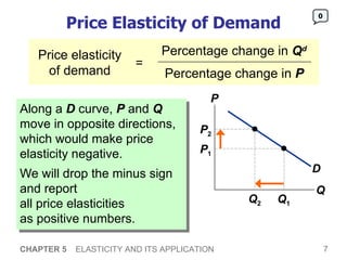
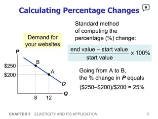
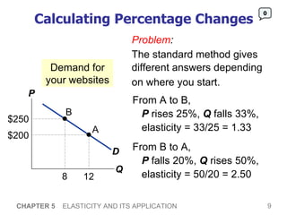
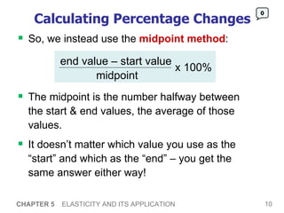
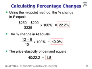
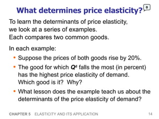
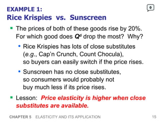
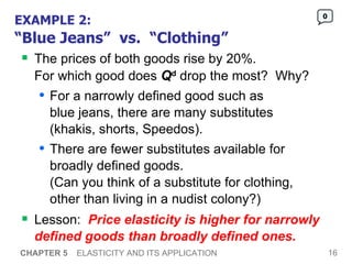
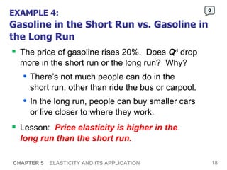
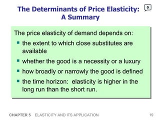
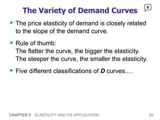
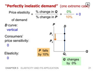
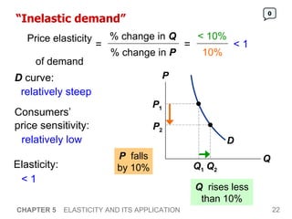
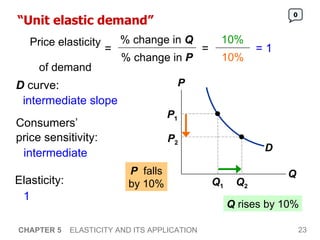
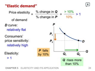
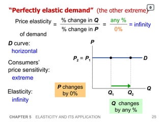
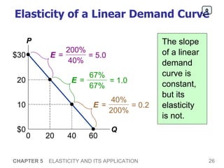
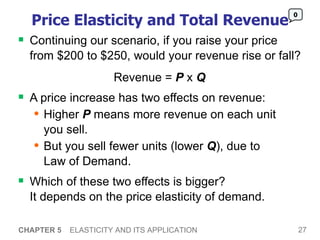
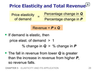
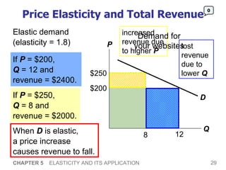
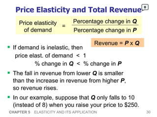
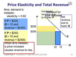
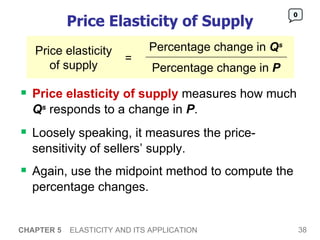
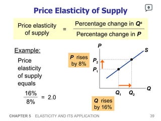
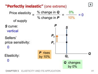
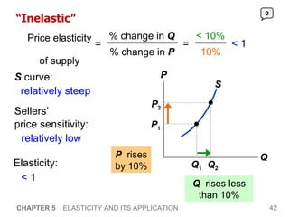
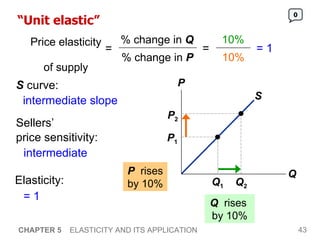
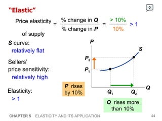
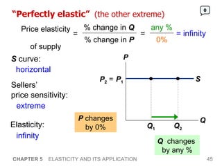
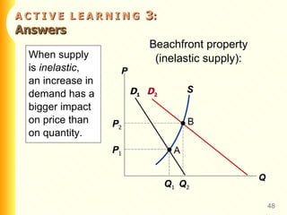
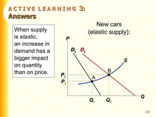
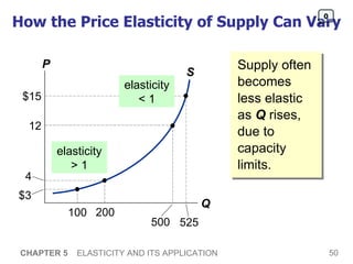
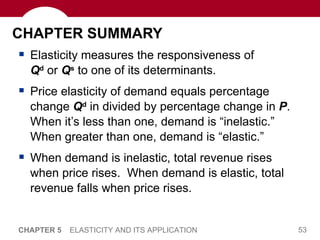
This chapter discusses elasticity, which measures how responsive one variable is to changes in another variable. It focuses on price elasticity of demand, which measures how much quantity demanded responds to changes in price. Price elasticity is calculated as the percentage change in quantity divided by the percentage change in price. Examples are used to illustrate factors that determine whether demand is elastic or inelastic, such as availability of substitutes. The elasticity also depends on whether a good is a necessity. The chapter explores how elasticity is related to the slope of the demand curve and total revenue.
This document discusses supply and demand. It begins by asking questions about factors that affect demand and supply, and how supply and demand determine price and quantity. It then defines markets and competition. The rest of the document discusses the concepts of demand, including demand schedules and curves. It explains individual demand versus market demand. It also discusses factors that can shift the demand curve, like number of buyers, income, prices of related goods, tastes, and expectations. Similarly, it covers the concepts of supply, including supply schedules and curves, as well as factors that shift the supply curve, like input prices, technology, number of sellers, and expectations. In summary, it provides an overview of the key microeconomic concepts of supply, demand,
This chapter discusses how government policies like price controls and taxes can affect market outcomes. Price ceilings, which set a legal maximum price, typically cause shortages by creating a gap between the maximum price and the market equilibrium price. Price floors, which set a legal minimum price, typically cause surpluses by creating a gap between the minimum price and the market equilibrium price. Taxes can be levied on buyers or sellers, but they have similar effects by driving a wedge between the price buyers pay and sellers receive. The incidence of a tax, or how the burden is shared, depends on the elasticities of supply and demand.
The document discusses the market forces of supply and demand. It defines demand and supply, and explains how demand and supply curves are determined by various factors. The demand curve shows the relationship between price and quantity demanded, while the supply curve shows the relationship between price and quantity supplied. The market reaches equilibrium when quantity demanded equals quantity supplied at the market price.
P
Q
D
$200
12
$250
10
1. The document discusses the concept of elasticity and how it can help understand how variables respond to changes in other variables.
2. It provides examples of different types of elasticities including price elasticity of demand, which measures how quantity demanded responds to changes in price. Demand is more elastic when good substitutes exist, a good is a luxury, the good is narrowly defined, or in the long run.
3. The slope of the demand curve is related to elasticity, with flatter curves indicating more elastic demand. Demand can be perfectly inelastic, inelastic, unit elastic, elastic, or
This chapter discusses the concept of interdependence and how trade between countries can make both countries better off. It uses an example of trade between the U.S. and Japan in computers and wheat. It shows that while the U.S. has an absolute advantage in both goods, Japan has a comparative advantage in computers when opportunity costs are considered. When each country specializes in the good it has a comparative advantage in and trades, both countries increase their consumption and are made better off through gains from trade. Comparative advantage, not just absolute advantage, is what allows for mutual benefits of trade between two countries.
This document discusses the costs of taxation according to microeconomic principles. It explains that a tax reduces consumer surplus, producer surplus, and total surplus by creating a deadweight loss. The size of the deadweight loss depends on the price elasticities of supply and demand - more elastic demand or supply leads to a larger deadweight loss. Increasing the size of an existing tax causes the deadweight loss to rise more than proportionately and causes tax revenue to initially rise and then fall, following a Laffer curve pattern.
Macroeconomics_Elasticity and its Applicationsdjalex035
This chapter discusses elasticity, which measures how responsive buyers and sellers are to changes in price. It defines price elasticity of demand as the percentage change in quantity demanded divided by the percentage change in price. Factors that make demand more elastic include availability of substitutes, whether a good is a necessity or luxury, how broadly the market is defined, and the time period considered. Price elasticity of supply is defined similarly for quantity supplied. Factors that make supply more elastic include the ability to change production and longer time periods. The chapter examines how elasticity relates to total revenue and applies elasticity concepts to different markets.
1) A perfectly competitive firm is a price taker and will produce the quantity where marginal revenue equals marginal cost to maximize profits.
2) In the short run, if price is below average variable cost the firm will shut down, and if below average total cost the firm will exit the market in the long run.
3) The market supply curve is determined by the marginal cost curves of all firms, and will be horizontal at the minimum of average total cost in the long run equilibrium with free entry and exit.
Mankiew chapter 7 Consumers, Producers, and the Efficiency of MarketsAbd ELRahman ALFar
What is consumer surplus? How is it related to the demand curve?
What is producer surplus? How is it related to the supply curve?
Do markets produce a desirable allocation of resources? Or could the market outcome be improved upon?
The document discusses the characteristics and behavior of firms in a perfectly competitive market. It defines a competitive market as having many small firms and buyers, homogeneous products, and free entry and exit. In the short run, individual firms maximize profits by producing where marginal revenue equals marginal cost. In the long run, firms enter and exit the market until price equals minimum average total cost and profits are zero. The market supply curve is determined by the marginal cost curves of individual firms.
This document discusses elasticity and its application in economics. It begins by asking questions about price elasticity of demand, price elasticity of supply, and other types of elasticities. It then provides an example scenario about a website designer considering raising their price from $200 to $250 per website. The document explains how to calculate percentage changes and elasticities using this scenario. It discusses how the price elasticity of demand relates to a demand curve's slope and total revenue. It also summarizes the key determinants of price elasticity and provides examples to illustrate these determinants. Finally, it discusses price elasticity of supply and provides an application example about drug interdiction policies.
This document provides an overview of the theory of consumer choice. It introduces key concepts like the budget constraint, indifference curves, marginal rate of substitution, and consumer optimization. The budget constraint represents the combinations of goods a consumer can afford based on prices and income. Indifference curves represent combinations of goods that provide equal utility. Consumers optimize by choosing the highest indifference curve possible given their budget constraint. The theory is then applied to explain consumer decisions around income and price changes, labor supply, and saving.
This document provides an overview of supply and demand in economics. It discusses key concepts like:
- Demand is affected by factors like price, income, tastes, and the prices of related goods. The demand curve shows the relationship between price and quantity demanded.
- Supply is affected by factors like input prices, technology, and the number of sellers. The supply curve shows the relationship between price and quantity supplied.
- Equilibrium price and quantity are determined by the intersection of supply and demand in the market. Changes in supply or demand shift the curves and result in a new equilibrium.
The document uses examples and diagrams to illustrate these concepts and how markets allocate resources through the interaction of supply and demand.
This chapter discusses supply and demand in markets. It will cover factors that affect demand and supply, how equilibrium price and quantity are determined, and how markets allocate resources. Key topics include the demand curve and how it shifts with changes in price, income, tastes; the supply curve and how it shifts with input prices, technology, number of sellers. The chapter analyzes how equilibrium is reached where quantity demanded equals quantity supplied and how surpluses and shortages occur away from equilibrium.
The document discusses the costs of taxation, including how taxes affect consumer surplus, producer surplus, and total surplus. It explains that the deadweight loss of a tax is the reduction in total surplus that results from the market distortion caused by the tax. The size of the deadweight loss depends on the price elasticities of supply and demand - the more elastic they are, the larger the deadweight loss will be. Doubling or tripling a tax causes the deadweight loss to increase by more than the amount of the tax increase. Tax revenue initially increases with tax size but eventually falls as the tax further reduces the size of the market.
1) The document discusses the characteristics and behavior of firms operating in perfectly competitive markets. It addresses factors like revenue, costs, and profit maximization.
2) A competitive firm is a price taker and will produce at the quantity where marginal revenue equals marginal cost, as this maximizes profits.
3) The marginal cost curve represents the firm's supply curve - at a higher price, the profit-maximizing quantity supplied increases as costs are covered at a greater output level.
This document discusses key concepts related to consumer surplus, producer surplus, and market efficiency. It asks questions about consumer surplus and its relationship to demand, producer surplus and its relationship to supply, and whether markets produce a desirable allocation of resources or if outcomes could be improved. The document then provides context on welfare economics and how the allocation of resources affects economic well-being.
This document discusses the concept of elasticity and its applications. It defines key terms like price elasticity of demand, price elasticity of supply, and total revenue. It examines how total revenue is affected by elasticity and provides examples to illustrate applications, including how good harvests can hurt farmers, why OPEC struggled to keep oil prices high, and how drug interdiction may increase short-run crime but decrease it long-run. The key points are that elasticity determines how quantities respond to price changes, and it is important for understanding how policies impact markets and different groups within them.
Economists use models like the circular flow diagram and production possibilities frontier (PPF) to study economic concepts. The circular flow diagram shows how resources and dollars flow between households and firms. The PPF illustrates production tradeoffs and opportunity costs given limited resources. Microeconomics analyzes individual markets, while macroeconomics examines economy-wide issues. Economists aim to explain the world scientifically and advise on policy normatively.
The document discusses consumer surplus, producer surplus, and how markets allocate resources efficiently. It defines:
- Consumer surplus as what consumers are willing to pay minus the price paid, and how it relates to the demand curve.
- Producer surplus as the price received minus costs of production, and how it relates to the supply curve.
- An efficient allocation as one that maximizes total surplus by having goods consumed by those valuing them most and produced by lowest cost producers.
The document evaluates an equilibrium in terms of efficiency using demand and supply curves to show buyers and sellers that transact value the good most and have lowest costs.
This document provides an overview of externalities and how they can lead to inefficient market outcomes. It discusses:
1) What externalities are and how they can be negative or positive, depending on their impact on third parties. Negative externalities like pollution mean the market produces too much of a good, while positive externalities mean too little is produced.
2) How public policies like taxes or subsidies can "internalize" externalities by making producers and consumers consider these external impacts. A tax on pollution would align private and social costs, leading to the efficient level of production.
3) Examples of both negative externalities like air pollution and positive externalities like vaccination. The document analyzes these situations using demand
A monopoly is a firm that is the sole seller of a product without close substitutes. It faces a downward-sloping demand curve and sets price above marginal cost. While a monopoly maximizes profits by producing where marginal cost equals marginal revenue, it produces less than the efficient quantity, resulting in deadweight loss. Governments address monopoly inefficiencies through antitrust laws, price regulation, or public ownership.
This document discusses monopolies and monopoly power. It defines a monopoly as a sole seller in a market that faces a downward-sloping demand curve. Monopolies maximize profits by producing where marginal cost equals marginal revenue. Unlike competitive firms, monopolies set price above marginal cost, resulting in deadweight loss. Governments address monopoly power through antitrust laws, price regulation, or public ownership.
This document outlines ten principles of economics according to N. Gregory Mankiw. It discusses how people make decisions by facing tradeoffs and considering opportunity costs. Rational people make decisions at the margin by weighing marginal costs against marginal benefits. Markets are generally an efficient way to organize economic activity as decentralized decisions lead to beneficial outcomes through the invisible hand of supply and demand.
Chapter 07 Consumers, Producers And The Efficiency Of Marketsira78
This chapter discusses consumer surplus, producer surplus, and how markets allocate resources efficiently. It defines key concepts like demand, supply, willingness to pay, and opportunity cost. The document analyzes an example market equilibrium and finds that it maximizes total surplus, allocating resources efficiently by having goods produced by low-cost sellers and consumed by buyers who value them most. The market outcome cannot be improved upon, suggesting governments should generally not interfere with free markets.
The document discusses the costs of production for a firm. It provides two examples:
1) Farmer Jack's wheat production, which shows how costs like labor wages and land rent contribute to total costs. Marginal product and costs are defined.
2) A general example of fixed, variable, and total costs. It shows how average costs like AFC, AVC, and ATC change with quantity and can be U-shaped. Marginal cost is also examined.
Marginal cost is the increase in total cost from producing one more unit of output. It is usually rising as quantity increases due to diminishing marginal productivity. Average total cost is total cost divided by quantity and is typically U-shaped as initially fixed costs are spread over more units but variable costs eventually increase faster than output. Understanding costs like marginal, average, fixed and variable helps firms determine optimal production levels to maximize profits.
CH-6 Supply, Demand, and Government Policies.pdfchhornqw
This document discusses how governments intervene in markets through policies like price controls and taxes. It provides examples of price ceilings, price floors, and taxes, and explains how each policy affects market outcomes. Specifically, it notes that a binding price ceiling below the equilibrium price causes a shortage, while a binding price floor above equilibrium causes a surplus. It also explains that a tax imposed on either buyers or sellers reduces the equilibrium quantity, and the incidence of the tax depends on supply and demand elasticities.
micro-ch05-presentation-120319214009-phpapp02 (1).pdfHaider Ali
This document discusses elasticity and its application to microeconomics. It begins by outlining key questions about elasticity, including the price elasticity of demand and supply and other elasticities. It then uses examples and scenarios to explain elasticity, determinants of price elasticity, the relationship between elasticity and total revenue/expenditure, and how elasticity can be applied to analyze policies. The document contains lecture slides on elasticity with definitions, formulas, graphs, and activities to help explain and apply elasticity concepts.
This document discusses elasticity and its application to economics. It begins by introducing the concept of elasticity and the different types, including price elasticity of demand. Price elasticity of demand measures the responsiveness of quantity demanded to a change in price. The document then uses an example of a business that designs websites to illustrate how to calculate price elasticity of demand numerically. It explores how the slope of the demand curve relates to elasticity. The document also examines the factors that determine the price elasticity of demand, such as availability of substitutes. It concludes by explaining how price elasticity relates to total revenue from price changes.
Falls, since demand for insulin is inelastic. While the price increases, quantity demanded will not decrease much. So the loss in expenditure from lower quantity will be less than the gain from the higher price, causing total expenditure to rise.
B. As a result of a fare war, the price of a luxury cruise falls 20%.
Does luxury cruise companies’ total revenue rise or fall?
Since a luxury cruise is a luxury good, demand is elastic.
A 20% price cut would cause a greater than 20% increase in quantity demanded.
So total revenue would rise.
If the website designer raises their price from $200 to $250 per website, total revenue would fall. Demand for websites is elastic, so quantity demanded would fall more than the 25% price increase. Specifically, quantity demanded would fall from 12 websites per month to 8. While the higher price increases revenue per website, the larger drop in quantity sold means total revenue falls from $2,400 to $2,000.
The document provides an overview of elasticity and its applications. It defines elasticity as a measure of how responsive one variable is to changes in another. It discusses the key concepts of price elasticity of demand, which measures how quantity demanded responds to price changes, and price elasticity of supply, which measures how quantity supplied responds to price changes. The document uses examples and scenarios to illustrate these concepts and how elasticity is related to the slope of demand and supply curves. It also discusses how elasticity can be used to determine whether total revenue will increase or decrease when price is changed.
Elasticity measures the responsiveness of one variable to changes in another. The document discusses different types of elasticity including:
1) Price elasticity of demand, which measures how much quantity demanded responds to changes in price. It is related to the slope of the demand curve.
2) Price elasticity of supply, which measures how much quantity supplied responds to price changes. It is related to the slope of the supply curve.
3) Other elasticities like income elasticity of demand and cross-price elasticity of demand are discussed. Income elasticity measures response of demand to income changes while cross-price elasticity measures response of one good's demand to price changes in another.
The document discusses the concept of price elasticity of demand. It provides examples to illustrate different types of elasticity:
1) Perfectly inelastic demand has a price elasticity of 0, meaning quantity demanded does not change when price changes.
2) Inelastic demand has a price elasticity below 1, indicating quantity demanded changes by a smaller percentage than the price change.
3) Unit elastic demand has a price elasticity of 1, where quantity demanded changes by the same percentage as the price change.
4) Elastic demand has a price elasticity above 1, so quantity demanded responds more than proportionately to price changes.
5) Perfectly elastic demand has an infinite price elasticity
The document discusses elasticity, specifically price elasticity of demand. It defines elasticity and explains how to calculate the price elasticity of demand using percentage changes in price and quantity. It provides examples of calculating price elasticity of demand values for different goods. It also categorizes goods based on their elasticity, such as inelastic, elastic, unit elastic and perfectly inelastic/elastic demands. Additional factors that can impact a good's elasticity are discussed such as availability of substitutes, necessities vs luxuries, the time horizon, and importance in a buyer's budget.
Presentation5 -principles of economics Kareem Hossam
This document discusses the concept of elasticity and how it relates to demand curves. It defines elasticity as measuring how responsive one variable is to changes in another. Specifically, it defines and provides examples of price elasticity of demand, which measures how much quantity demanded responds to changes in price. Factors that determine the price elasticity of demand include availability of substitutes, whether the good is a necessity or luxury, and how broadly or narrowly the good is defined. The document also discusses the implications of elastic versus inelastic demand on total revenue from price changes.
1. Elasticity measures the responsiveness of quantity demanded or supplied to changes in factors like price. Price elasticity of demand specifically measures how much quantity demanded responds to changes in price. Price elasticity of supply measures how much quantity supplied responds to price changes.
2. Calculating elasticities involves determining the percentage changes in quantity and price and taking the ratio. Demand can be elastic, inelastic, or unit elastic depending on whether the elasticity is greater than, less than, or equal to one.
3. Whether a price increase raises or lowers total revenue depends on whether demand is elastic or inelastic. An elastic demand means revenue falls with a price increase while an inelastic demand means revenue rises
The document discusses various types of elasticity, including price elasticity of demand, price elasticity of supply, income elasticity of demand, and cross elasticity. It provides examples of how to calculate elasticity coefficients from changes in price and quantity. Specifically, it examines how price elasticity indicates whether a change in price will increase or decrease total revenue, depending on whether demand is elastic, inelastic, or unit elastic. The document also discusses how cross elasticity is positive for substitute goods and negative for complementary goods.
This document discusses the concept of elasticity in economics, including price elasticity of demand, price elasticity of supply, cross elasticity, and income elasticity. It provides definitions and formulas for calculating each type of elasticity. Examples are given to illustrate how to compute elasticity coefficients and determine whether two products are substitutes, complements, or unrelated based on cross elasticity. The document also examines the total revenue test and how total revenue moves in relation to price changes depending on whether demand is elastic or inelastic.
The document discusses different types of elasticity of demand including price elasticity, income elasticity, cross elasticity, substitution elasticity, and advertising elasticity. It defines each type and provides formulas for measuring elasticity. Some key points include:
- Price elasticity measures the responsiveness of demand to a change in price. It can be perfectly elastic, unitary, or perfectly inelastic.
- Income elasticity indicates whether a good is a necessity or luxury based on whether demand increases or decreases with income.
- Cross elasticity captures the relationship between the demand for one good and the price of another good, such as substitutes or complements.
- Substitution elasticity measures how easily consumers can substitute one
The document discusses price elasticity of demand and how it is calculated. It provides examples of goods that are elastic or inelastic, as well as extreme cases of perfectly inelastic, unit elastic, and perfectly elastic demand. Price elasticity is calculated using the percentage change in quantity demanded divided by the percentage change in price. It must be measured using the midpoint method to avoid inconsistent results. The elasticity indicates how responsive consumers are to price changes.
This document provides an overview of key concepts related to elasticity of demand and supply including:
- Price elasticity of demand measures the responsiveness of quantity demanded to a price change. Demand is elastic when a price increase reduces total revenue and inelastic when it increases total revenue.
- Supply is more elastic over time as producers can adjust production levels. Demand becomes more elastic as consumers have more substitutes and time to adjust to price changes.
- Complements have negative cross-price elasticity while substitutes have positive cross-price elasticity. Income elasticity is positive for normal goods and negative for inferior goods.
- Perfectly elastic and inelastic demand curves are horizontal and vertical lines
Chapter. 5 elasticity by Mankiw Economics .pdfprottoy21306011
Elasticity allows for more precise analysis of supply and demand. It measures how buyers and sellers respond to changes in market conditions. The document discusses the price elasticity of demand and supply, as well as the determinants and calculations of elasticity. It also covers applications of elasticity, such as how a new wheat hybrid could impact wheat farmers through shifts in the supply curve.
Elasticity measures the responsiveness of one variable to changes in another. There are several types of elasticity including price elasticity of demand, income elasticity of demand, and price elasticity of supply. Price elasticity of demand compares the percentage change in quantity demanded to a percentage change in price. Income elasticity of demand compares the percentage change in demand to a percentage change in income. Price elasticity of supply compares the percentage change in quantity supplied to a percentage change in price. Elasticity estimates help predict how consumers and producers will respond to market changes.
Elasticity measures the responsiveness of one variable to changes in another variable. There are different types of elasticity including price elasticity of demand, which measures the responsiveness of quantity demanded to changes in price. Elasticity is computed as a ratio of percentage changes and has no units. Demand is elastic if the elasticity value is greater than 1, inelastic if less than 1, and unit elastic if equal to 1. The elasticity between two points on a demand curve can differ even if the slope is the same.
A workshop hosted by the South African Journal of Science aimed at postgraduate students and early career researchers with little or no experience in writing and publishing journal articles.
A review of the growth of the Israel Genealogy Research Association Database Collection for the last 12 months. Our collection is now passed the 3 million mark and still growing. See which archives have contributed the most. See the different types of records we have, and which years have had records added. You can also see what we have for the future.
Macroeconomics- Movie Location
This will be used as part of your Personal Professional Portfolio once graded.
Objective:
Prepare a presentation or a paper using research, basic comparative analysis, data organization and application of economic information. You will make an informed assessment of an economic climate outside of the United States to accomplish an entertainment industry objective.
A Strategic Approach: GenAI in EducationPeter Windle
Artificial Intelligence (AI) technologies such as Generative AI, Image Generators and Large Language Models have had a dramatic impact on teaching, learning and assessment over the past 18 months. The most immediate threat AI posed was to Academic Integrity with Higher Education Institutes (HEIs) focusing their efforts on combating the use of GenAI in assessment. Guidelines were developed for staff and students, policies put in place too. Innovative educators have forged paths in the use of Generative AI for teaching, learning and assessments leading to pockets of transformation springing up across HEIs, often with little or no top-down guidance, support or direction.
This Gasta posits a strategic approach to integrating AI into HEIs to prepare staff, students and the curriculum for an evolving world and workplace. We will highlight the advantages of working with these technologies beyond the realm of teaching, learning and assessment by considering prompt engineering skills, industry impact, curriculum changes, and the need for staff upskilling. In contrast, not engaging strategically with Generative AI poses risks, including falling behind peers, missed opportunities and failing to ensure our graduates remain employable. The rapid evolution of AI technologies necessitates a proactive and strategic approach if we are to remain relevant.
June 3, 2024 Anti-Semitism Letter Sent to MIT President Kornbluth and MIT Cor...Levi Shapiro
Letter from the Congress of the United States regarding Anti-Semitism sent June 3rd to MIT President Sally Kornbluth, MIT Corp Chair, Mark Gorenberg
Dear Dr. Kornbluth and Mr. Gorenberg,
The US House of Representatives is deeply concerned by ongoing and pervasive acts of antisemitic
harassment and intimidation at the Massachusetts Institute of Technology (MIT). Failing to act decisively to ensure a safe learning environment for all students would be a grave dereliction of your responsibilities as President of MIT and Chair of the MIT Corporation.
This Congress will not stand idly by and allow an environment hostile to Jewish students to persist. The House believes that your institution is in violation of Title VI of the Civil Rights Act, and the inability or
unwillingness to rectify this violation through action requires accountability.
Postsecondary education is a unique opportunity for students to learn and have their ideas and beliefs challenged. However, universities receiving hundreds of millions of federal funds annually have denied
students that opportunity and have been hijacked to become venues for the promotion of terrorism, antisemitic harassment and intimidation, unlawful encampments, and in some cases, assaults and riots.
The House of Representatives will not countenance the use of federal funds to indoctrinate students into hateful, antisemitic, anti-American supporters of terrorism. Investigations into campus antisemitism by the Committee on Education and the Workforce and the Committee on Ways and Means have been expanded into a Congress-wide probe across all relevant jurisdictions to address this national crisis. The undersigned Committees will conduct oversight into the use of federal funds at MIT and its learning environment under authorities granted to each Committee.
• The Committee on Education and the Workforce has been investigating your institution since December 7, 2023. The Committee has broad jurisdiction over postsecondary education, including its compliance with Title VI of the Civil Rights Act, campus safety concerns over disruptions to the learning environment, and the awarding of federal student aid under the Higher Education Act.
• The Committee on Oversight and Accountability is investigating the sources of funding and other support flowing to groups espousing pro-Hamas propaganda and engaged in antisemitic harassment and intimidation of students. The Committee on Oversight and Accountability is the principal oversight committee of the US House of Representatives and has broad authority to investigate “any matter” at “any time” under House Rule X.
• The Committee on Ways and Means has been investigating several universities since November 15, 2023, when the Committee held a hearing entitled From Ivory Towers to Dark Corners: Investigating the Nexus Between Antisemitism, Tax-Exempt Universities, and Terror Financing. The Committee followed the hearing with letters to those institutions on January 10, 202
This presentation includes basic of PCOS their pathology and treatment and also Ayurveda correlation of PCOS and Ayurvedic line of treatment mentioned in classics.
Thinking of getting a dog? Be aware that breeds like Pit Bulls, Rottweilers, and German Shepherds can be loyal and dangerous. Proper training and socialization are crucial to preventing aggressive behaviors. Ensure safety by understanding their needs and always supervising interactions. Stay safe, and enjoy your furry friends!
This presentation was provided by Steph Pollock of The American Psychological Association’s Journals Program, and Damita Snow, of The American Society of Civil Engineers (ASCE), for the initial session of NISO's 2024 Training Series "DEIA in the Scholarly Landscape." Session One: 'Setting Expectations: a DEIA Primer,' was held June 6, 2024.
Executive Directors Chat Leveraging AI for Diversity, Equity, and InclusionTechSoup
Let’s explore the intersection of technology and equity in the final session of our DEI series. Discover how AI tools, like ChatGPT, can be used to support and enhance your nonprofit's DEI initiatives. Participants will gain insights into practical AI applications and get tips for leveraging technology to advance their DEI goals.
Executive Directors Chat Leveraging AI for Diversity, Equity, and Inclusion
Princ ch05-presentation
1. 5 Elasticity and its Application P R I N C I P L E S O F F O U R T H E D I T I O N
2.
3.
4.
5.
6.
7.
8. Calculating Percentage Changes CHAPTER 5 ELASTICITY AND ITS APPLICATION 0 Deman d for your websites Standard method of computing the percentage (%) change: Going from A to B, the % change in P equals ($250–$200)/$200 = 25% P Q D $250 8 B $200 12 A end value – start value start value x 100%
9. Calculating Percentage Changes CHAPTER 5 ELASTICITY AND ITS APPLICATION 0 Deman d for your websites Problem : The standard method gives different answers depending on where you start. From A to B, P rises 25%, Q falls 33%, elasticity = 33/25 = 1.33 From B to A, P falls 20%, Q rises 50%, elasticity = 50/20 = 2.50 P Q D $250 8 B $200 12 A
10.
11.
12.
13.
14.
15.
16.
17.
18.
19.
20.
21. “ Perfectly inelastic demand” (one extreme case) CHAPTER 5 ELASTICITY AND ITS APPLICATION P falls by 10% Q changes by 0% 0 0% 10% = 0 Consumers’ price sensitivity: D curve: Elasticity: vertical 0 0 Q 1 P 1 D P Q P 2 Price elasticity of demand = % change in Q % change in P =
22. “ Inelastic demand” CHAPTER 5 ELASTICITY AND ITS APPLICATION Q rises less than 10% 0 < 10% 10% < 1 P falls by 10% Consumers’ price sensitivity: D curve: Elasticity: relatively steep relatively low < 1 D P Q Q 1 P 1 Q 2 P 2 Price elasticity of demand = % change in Q % change in P =
23. “ Unit elastic demand” CHAPTER 5 ELASTICITY AND ITS APPLICATION Q rises by 10% 0 10% 10% = 1 P falls by 10% Consumers’ price sensitivity: Elasticity: intermediate 1 D curve: intermediate slope D P Q Q 1 P 1 Q 2 P 2 Price elasticity of demand = % change in Q % change in P =
24. “ Elastic demand” CHAPTER 5 ELASTICITY AND ITS APPLICATION Q rises more than 10% 0 > 10% 10% > 1 P falls by 10% Consumers’ price sensitivity: D curve: Elasticity: relatively flat relatively high > 1 D P Q Q 1 P 1 Q 2 P 2 Price elasticity of demand = % change in Q % change in P =
25. “ Perfectly elastic demand” (the other extreme) CHAPTER 5 ELASTICITY AND ITS APPLICATION P 1 P changes by 0% Q changes by any % 0 any % 0% = infinity P 2 = Consumers’ price sensitivity: D curve: Elasticity: infinity horizontal extreme D P Q Q 1 Q 2 Price elasticity of demand = % change in Q % change in P =
26.
27.
28.
29.
30.
31.
32.
33.
34.
35.
36. Policy 1: Interdiction CHAPTER 5 ELASTICITY AND ITS APPLICATION 0 Interdiction reduces the supply of drugs. Since demand for drugs is inelastic, P rises propor-tionally more than Q falls. Result: an increase in total spending on drugs, and in drug-related crime D 1 Price of Drugs Quantity of Drugs S 1 S 2 P 1 Q 1 P 2 Q 2 new value of drug-related crime initial value of drug-related crime
37. Policy 2: Education CHAPTER 5 ELASTICITY AND ITS APPLICATION 0 Education reduces the demand for drugs. P and Q fall. Result: A decrease in total spending on drugs, and in drug-related crime. Price of Drugs Quantity of Drugs D 1 S P 1 Q 1 D 2 P 2 Q 2 initial value of drug-related crime new value of drug-related crime
38.
39.
40.
41. “ Perfectly inelastic” (one extreme) CHAPTER 5 ELASTICITY AND ITS APPLICATION Q 1 P 1 Q changes by 0% 0 0% 10% = 0 P rises by 10% Sellers’ price sensitivity: S curve: Elasticity: vertical 0 0 S P Q P 2 Price elasticity of supply = % change in Q % change in P =
42. “ Inelastic” CHAPTER 5 ELASTICITY AND ITS APPLICATION Q 1 P 1 Q rises less than 10% 0 < 10% 10% < 1 P rises by 10% Sellers’ price sensitivity: S curve: Elasticity: relatively steep relatively low < 1 S P Q Q 2 P 2 Price elasticity of supply = % change in Q % change in P =
43. “ Unit elastic” CHAPTER 5 ELASTICITY AND ITS APPLICATION Q 1 P 1 Q rises by 10% 0 10% 10% = 1 P rises by 10% Sellers’ price sensitivity: S curve: Elasticity: intermediate slope intermediate = 1 S P Q Q 2 P 2 Price elasticity of supply = % change in Q % change in P =
44. “ Elastic” CHAPTER 5 ELASTICITY AND ITS APPLICATION Q 1 P 1 Q rises more than 10% 0 > 10% 10% > 1 P rises by 10% Sellers’ price sensitivity: S curve: Elasticity: relatively flat relatively high > 1 S P Q Q 2 P 2 Price elasticity of supply = % change in Q % change in P =
45. “ Perfectly elastic” (the other extreme) CHAPTER 5 ELASTICITY AND ITS APPLICATION P 1 P changes by 0% Q changes by any % 0 any % 0% = infinity P 2 = Sellers’ price sensitivity: S curve: Elasticity: horizontal extreme infinity S P Q Q 1 Price elasticity of supply = % change in Q % change in P = Q 2
46.
47.
48.
49.
50.
51.
52.
53.
54.
55.
Editor's Notes
The elasticity chapter in most principles textbooks is fairly technical, and is not always students’ favorite. This PowerPoint chapter contains several special features designed to engage and motivate students to learn this important material. First, we consider a scenario in which students face a business decision – whether to raise the price of a service they sell. This scenario is used to illustrate the effects of raising price on number of units sold and on revenue, which students immediately recognize as critical to the business decision. Second, instead of merely listing the determinants of elasticity, students are asked to think about some concrete examples and deduce from each one a lesson about the determinants of elasticity. Third, instead of putting the applications at the end of the chapter (as in the textbook), this PowerPoint includes one of them immediately after the section on price elasticity of demand. This helps break up what would otherwise be a long stretch of theory. Please be assured that this PowerPoint presentation is, nonetheless, very consistent with the textbook’s approach.
We will follow this scenario throughout the first section of this chapter (the section on price elasticity of demand) to illustrate and motivate several important concepts, such as the impact of price changes on sales and revenue.
Here, Q d and Q s are short for quantity demanded and quantity supplied, as in the PowerPoint for Chapter 4.
It might be worth explaining to your students that “P and Q move in opposite directions” means that the percentage change in Q and the percentage change in P will have opposite signs, thus implying a negative price elasticity. To be consistent with the text, the last statement in the green box says that we will report all price elasticities as positive numbers. It might be slightly more accurate to say that we will report all elasticities as non-negative numbers: we want to allow for the (admittedly rare) case of zero elasticity.
These calculations are based on the example shown a few slides back: points A and B on the website demand curve.
In essence, the textbook says “Here are the determinants of elasticity. The first one is availability of close substitutes. Here’s an example….” That’s great for a textbook. For teaching, I’ve found a different approach to be far more effective: having students deduce the general lessons from specific examples they can figure out using common sense. This is the approach on the next few slides. Also, see notes on the next slide for a good suggestion.
Suggestion: For each of these examples, display the slide title (which lists the two goods) and the first two lines of text (which ask which good experiences the biggest drop in demand in response to a 20% price increase). Give your students a quiet minute to formulate their answers. Then, ask for volunteers.
You might need to clarify the nature of this thought experiment. Here, we look at two alternate scenarios. In the first, the price of blue jeans (and no other clothing) rises by 20%, and we observe the percentage decrease in quantity of blue jeans demanded. In the second scenario, the price of all clothing rises by 20%, and we observe the percentage decrease in demand for all clothing.
This slide is a convenience for your students, and replicates a similar table from the text. If you’re pressed for time, it is probably safe to omit this slide from your presentation.
Economists classify demand curves according to their elasticity. The next 5 slides present the five different classifications, from least to most elastic.
If Q doesn’t change, then the percentage change in Q equals zero, and thus elasticity equals zero. It is hard to think of a good for which the price elasticity of demand is literally zero. Take insulin, for example. A sufficiently large price increase would probably reduce demand for insulin a little, particularly among people with very low incomes and no health insurance. However, if elasticity is very close to zero, then the demand curve is almost vertical. In such cases, the convenience of modeling demand as perfectly inelastic probably outweighs the cost of being slightly inaccurate.
An example: student demand for textbooks that their professors have required for their courses. Here, it’s a little more clear that elasticity would be small, but not zero. At a high enough price, some students will not buy their books, but instead will share with a friend, or try to find them in the library, or just take copious notes in class. Another example: gasoline in the short run.
This is the intermediate case: the demand curve is neither relatively steep nor relatively flat. Buyers are neither relatively price-sensitive nor relatively insensitive to price. This is also the case where price changes have no effect on revenue.
A good example here would be Rice Krispies, or nearly anything with readily available substitutes. An elastic demand curve is flatter than a unit elastic demand curve (which itself is flatter than an inelastic demand curve).
“ Extreme price sensitivity” means the tiniest price increase causes demand to fall to zero. “ Q changes by any %” – when the D curve is horizontal, quantity cannot be determined from price. Consumers might demand Q1 units one month, Q2 units another month, and some other quantity later. Q can change by any amount, but P always “changes by 0%” (i.e. doesn’t change). If perfectly inelastic is one extreme, this (perfectly elastic) is the other. Here’s a good real-world example of a perfectly elastic demand curve, which foreshadows an upcoming chapter on firms in competitive markets. Suppose you run a small family farm in Iowa. Your main crop is wheat. The demand curve in this market is downward-sloping, and the market demand and supply curves determine the price of wheat. Suppose that price is $5/bushel. Now consider the demand curve facing you, the individual wheat farmer. If you charge a price of $5, you can sell as much or as little as you want. If you charge a price even just a little higher than $5, demand for YOUR wheat will fall to zero: Buyers would not be willing to pay you more than $5 when they could get the same wheat elsewhere for $5. Similarly, if you drop your price below $5, then demand for YOUR wheat will become enormous (not literally infinite, but “almost infinite”): if other wheat farmers are charging $5 and you charge less, then EVERY buyer will want to buy wheat from you. Why is the demand curve facing an individual producer perfectly elastic? Recall that elasticity is greater when lots of close substitutes are available. In this case, you are selling a product that has many perfect substitutes: the wheat sold by every other farmer is a perfect substitute for the wheat you sell.
The material on this slide is not used anywhere else in the textbook. Therefore, if you are pressed for time and looking for things to cut, you might consider cutting this slide. (Note that this is my personal recommendation and is not necessarily the official position of Greg Mankiw or Thomson/South-Western.) Due to space limitations, this slide uses “E” as an abbreviation for elasticity, or more specifically, the price e lasticity of demand, and the slide omits the analysis of revenue along the demand curve. Calculations of percentage changes use the midpoint method. (This is why the increase from Q=0 to Q=20 is 200% rather than infinity.) As you move down a linear demand curve, the slope (the ratio of the absolute change in P to that in Q) remains constant: From the point (0, $30) to the point (20, $20), the “rise” equals -$10, the “run” equals +20, so the slope equals -1/2 or -0.5. From the point (40, $10) to the point (60, $0), the “rise” again equals -$10, the “run” equals +20, and the slope again equals -0.5. However, the percentage changes in these variables do not remain constant, as shown by the different colored elasticity calculations that appear on the slide. The lesson here is that elasticity falls as you move downward & rightward along a linear demand curve.
We return to our scenario. It’s not hard for students to imagine being in this position – running their own business and trying to decide whether to raise the price. To most of your students, it should be clear that making the best possible decision would require information about the likely effects of the price increase on revenue. That is why elasticity is so helpful, as we will now see….
In the “Normal” view (edit mode), the labels over the graph look cluttered, like they’re on top of each other. This is not a mistake – in “Slide Show” mode (presentation mode), they will be fine – try it! Point out to students that the area (outlined in blue) representing lost revenue due to lower Q is larger than the area (outlined in yellow) representing increased revenue due to higher P. Hence, the net effect is a fall in revenue.
Again, the slide appears cluttered in “Normal” view (edit mode), but everything is fine when displayed in “Slide Show” mode (presentation mode). Point out to students that the area representing lost revenue due to lower Q is smaller than the area representing increased revenue due to higher P. Hence, the net effect is an increase in revenue. The knife-edge case, not shown here but perhaps worth mentioning in class, is unit-elastic demand. In that case, an increase in price leaves revenue unchanged: the increase in revenue from higher P exactly offsets the lost revenue due to lower Q.
These problems, perhaps similar to those you might ask on an exam, are complex in that they test several skills at once: Students must determine whether demand for each good is elastic or inelastic, and they must determine the impact of a price change on revenue/expenditure. So far, we’ve been talking about how elasticity determines the effects of an increase in P on revenue. Part (b) asks your students to determine the effects of a decrease in P.
The first part of the explanation discusses the opposing effects on revenue; its purpose is to clarify the effects of a price decrease on revenue, as we have previously only discussed the effects of a price increase.
In the textbook, this application appears near the end of the chapter, and you can easily move these slides to the end if you wish to teach things in the same order as the book. However, I encourage you to consider teaching this application right here - immediately after the section on price elasticity of demand. It is safe to do so, as this application only requires knowledge of price elasticity of demand. Also, putting the application here breaks up what would otherwise be a very long section of theory with a real-world example that most students find very interesting. Knowing elasticity helps us understand what might otherwise be a counter-intuitive result (that drug interdiction increases drug-related crime rather than reducing it).
By the time all elements have appeared on the screen, the slide will look kind of busy. I think this is okay, because the elements appear on the screen one by one, so students have time to absorb each one before the next one appears. However, if you’d rather strip the slide down a bit, here’s a suggestion: in “Normal” view (which is used to edit slides), you can delete the boxes that represent the initial and new values of drug-related crime, and the accompanying captions. Then, when presenting this slide in class, simply point out (with your mouse cursor, a laser pointer, or even your arms and hands) the areas that represent the initial and new values of drug-related crime.
Most everything in the “price elasticity of supply” section corresponds to analogous concepts from the “price elasticity of demand” section. So, it is probably safe to move through this section more quickly.
Economists classify supply curves according to their elasticity. The next 5 slides present the different classifications, from least to most elastic.
This section is not perfectly analogous to the section on the determinants of the price elasticity of demand, but it’s similar enough that you can probably cover it more quickly and with less hand-holding.
This is one of the “Problems and Applications” at the end of the chapter.
In this slide and the next, the initial price and quantity and the two demand curves are the same. The only difference is the elasticity of supply and slope of the supply curve. [The D curve shifts to the right, but not in a parallel fashion: at each price, quantity demanded is twice as high, so the new D curve will be flatter than the initial one.] In the text box containing the verbal explanation, “bigger impact” is shorthand for “bigger percentage impact” or “bigger proportional impact.”
This graph replicates the one in Figure 6. Note: The graph here is not quite drawn to scale. When the price rises from $3 to $4 (a 29% increase, using the midpoint method), quantity rises from 100 to 120 (or 67%). Because 67% > 29%, price elasticity of supply is greater than one. When the price rises from $12 to $15 (22%), quantity rises from 500 to 525 (about 5%), so price elasticity of supply is less than one. The way I like to explain this is as follows: When output is very low, it is relatively easy for firms to increase output. They may have excess capacity, or they are not requiring full effort from their workers. Increasing output is not difficult, so it doesn’t take much of an increase in price to induce an increase in production. When output is very high, it is relatively expensive for firms to increase output further: there’s little or no excess capacity, they are already running their factories and machines at a high level of intensity. To increase output further, they might have to pay their workers overtime, and their machines experience more wear and tear and therefore require more repairs. So, at high levels of output, it takes a much larger price increase to make firms willing to increase output further. Eventually, firms bump up against their capacity constraints, and simply cannot increase output in response to further price increases. Of course, all of this applies to the short run. In the long run, firms can build more factories, and (depending on the market structure) new firms can enter the market.
This topic and the next one (cross-price elasticity) do not appear anywhere else in the book. Instructors who are pressed for time may consider cutting these topics. (This is merely my suggestion, not the official position of Greg Mankiw or Thomson/South-Western.)